Throughput Prediction of 5G Network Based on Trace Similarity for Adaptive Video

Abstract

Predicting throughput is essential to reduce latency in time-critical services like video streaming, which constitutes a significant portion of mobile network traffic. The video player continuously monitors network throughput during playback and adjusts the video quality according to the network conditions. This means that the quality of the video depends on the player’s ability to predict network throughput accurately, which can be challenging in the unpredictable environment of mobile networks. To improve the prediction accuracy, we grouped the throughput trace into clusters taking into account the similarity of their mean and variance. Once we distinguished the similar trace fragments, we built a separate LSTM predictive model for each cluster. For the experiment, we used traffic captured from 5G networks generated by individual user equipment (UE) in fixed and mobile scenarios. Our results show that the prior grouping of the network traces improved the prediction compared to the global model operating on the whole trace.

1. Introduction

Cellular networks have been improving rapidly over the last few decades. The latest 5G systems are designed to offer faster data transfer speeds and lower network latency than earlier generations. However, some experts say that limitations in the underlying technology, including devices and wired internet access, may reduce these potential benefits [1]. Additionally, current wireless protocols are not optimized for the unique conditions of cellular networks, leading to the underutilization of available bandwidth [2]. This can be particularly problematic for multimedia applications like dynamic adaptive streaming over HTTP (DASH), where demand often exceeds available resources.

The predictability of network throughput can improve the performance of upper-layer protocols and network applications. In the abovementioned DASH, a video player periodically downloads segments, concatenates them, and delivers a continuous video stream to the user. During video playback, the player can request different segment versions to adjust the bit rate based on predicted network conditions. If the prediction is not accurate, the streaming algorithms will either be too conservative and download a lower-quality video than necessary or be too aggressive and download a video of higher quality, which will result in the video freezing at a certain time point in the future. Therefore, the more accurate the prediction, the better the quality of the user’s experience [3].

Typically, a DASH application measures the throughput after downloading each video segment. Hence, the video player decides on the video quality at intervals longer than the length of a downloaded video segment, which is usually between 2 and 10 s of video. For example, the Microsoft Smooth Streaming algorithm uses 2–5 s [4]. Therefore, to make our results suitable for this type of service, we tried to predict the average throughput in the next 4 s, with a trace of historical throughput measured every 4 s.

The variability of wireless transmission, such as changes in signal strength, interference, noise, and user movement, can result in highly unpredictable data transfer rates. The radio environment is dynamic, and even small changes in distance can significantly alter its properties [5]. Because of this, the throughput of wireless networks can fluctuate rapidly due to various random factors, including environmental conditions. Traditional models such as ARIMA cannot accurately predict the relationship between these factors and throughput. Additionally, prediction algorithms based on ANNs may not outperform simpler models unless the underlying data are extensive enough to fit complex models. Even if we capture sufficient amounts of past network throughput, its statistical properties and patterns can be altered by, e.g., a changing user equipment (UE) location, other UE joining the same cell, moving objects, or changing weather [6]. In this environment, the predictive model struggles with non-stationarity and concept drift. It repeatedly needs to reformulate its decision boundaries, to the detriment of the prediction accuracy.

Our contribution is to overcome this shortcoming by the following:

• Building separate models for the groups of times series representing the throughput;
• Constructing automatically the subgroups using similarities in the trace measured by a moving average and a variance.

Contrary to the works employing clustering and prediction, we do not compare or group multiple traces but search for similarities within each trace separately. Also, contrary to other research, to cluster the traces, we do not compare them directly but use for this purpose their statistical features. Then, we train separate LSTM ANNs for each group individually. When predicting a new value, before we feed data into an LSTM unit, we select the model that best matches the characteristics of the input vector.

In the Section 2, we describe the problems of network traffic prediction with examples from selected works. In Section 3, we present the workflow of our experiment, which includes capturing the network traffic, feature extraction, clustering, and developing an LSTM-based predictive model. Finally, in Section 4, we show and discuss the results. The Section 5 concludes the paper.

2. Related Works

Network traffic prediction is a useful solution that can help with various challenges in networking such as resource provisioning, congestion detection, and fault tolerance. In the past two decades, researchers have shifted their focus from predicting Internet traffic generated by a range of applications to predicting single or multiple flows within mobile wireless networks. However, predicting single traffic flows in an unstable mobile environment presents a significant challenge due to the high variability and outliers compared to an aggregated trace smoothed by statistical multiplexing [7]. In addition, DASH systems that stream video segments in an ON–OFF fashion create bursts in transmission, leading to even more complex patterns.

Traffic prediction involves using different models and techniques depending on the type of network and its purpose. In the past, researchers and network engineers used statistics-related techniques to analyse data patterns without prior knowledge or model training. These techniques are simple to use, have low computational overhead, and can handle a limited number of features. They usually compare the current data pattern with the last identified pattern to determine possible changes or predict future points in the time series based on the lagged data. However, these traditional methods cannot capture complex dependencies in large datasets and have limitations when dealing with non-stationary time series. Nowadays, machine learning (ML) methods are used in conjunction with or in opposition to traditional methods. However, there is still room for improvement in terms of efficiency, performance, computational burden, and training. There is also an ongoing debate about their accuracy and computational requirements [8]. A comprehensive overview of statistical and ML approaches to network traffic prediction can be found in [9].

In the past decade, deep learning models have made significant progress and have achieved remarkable success in various areas. With a sizeable and diverse dataset, machine learning algorithms can learn to recognize intricate non-linear patterns and discover unstructured relationships without having to make assumptions ahead of time. This means that ML algorithms are not constrained by preconceived notions or predetermined data-generating procedures, which allows the data to reveal their insights. However, the superiority of ML is not apparent when it comes to network traffic forecasting, as some research has reported that feed-forward ANNs and ARIMA could provide better performance than deep ANNs [10].

The literature on network throughput prediction is extensive and can be classified into several domains. Firstly, we can distinguish between low and high time aggregation scales for the network traffic. The boundary between the scales is subjective, and there are works that set the prediction horizon to milliseconds [7,11], seconds [3], minutes [12], and hours [13]. We focus on the seconds scale, where the LSTM ANN and its variant are often selected for prediction. Most works have focused on higher aggregation scales because the prediction is simpler, as the traffic is smoother, has seasonal components, and has fewer outliers. An example of a work incorporating low aggregated traffic is [14], which analysed downlink and uplink throughput generated by remotely controlled vehicles in LTE and 5G networks. Besides LSTM networks, another popularly employed method for the low aggregation scale is Random Forest. As per the study conducted by Labonne et al. [15], the Random Forest model is more effective in flow throughput prediction as compared to a deep ANN. The study tested various time windows ranging from 0.03 s to 4 s on nearly one million flows consisting of traces from various networks and applications. In addition to flow history data, the study also considered other attributes related to TCP such as window size, window scale, and segment retransmissions.

Secondly, prediction can also be a single step, e.g., [16], or multiple steps, e.g., [13]. Multistep analysis is more challenging and is usually applied to forecast more aggregated traffic with a longer time horizon. In this paper, we use single-step prediction. Multistep prediction would be more beneficial, as a DASH system could make more far-fetched decisions and avoid too frequent changes in video quality. However, such a prediction would be very challenging and subjected to a significant error.

Thirdly, many works have considered the spatial characteristics of mobile networks, including traffic generated by multiple base stations (BSs). This approach aims to enhance traffic prediction by exploiting the correlation between traffic flows across neighbouring BSs generated by users’ continuous movement within the network [17,18,19]. The spatial modelling of traffic flow has several challenges. One issue is data collection. The point of the network at which to capture the traffic in order to obtain the characteristics of the traffic flow in the system is an open question. It is important to note that relying on a few fixed measurement points may not accurately capture the radio environment at different locations [20]. The radio environment can vary significantly within just a few meters, so it is unclear how reliable these measurement points are in predicting throughput for mobile devices that frequently change radio environments [21]. While monitoring multiple UE devices can help, it also has limitations. For example, reporting UE geographic coordinates raises privacy concerns, and transmitting radio measurements from a UE to a BS would increase system traffic, leading to less accurate predictions.

Many works have considered both upper- and lower-layer information when predicting link bandwidth, as relying solely on historical throughput can result in inferior performance. Using all available features is known as multivariate prediction, while only considering a single feature, such as throughput, is univariate prediction. Therefore, combining multiple features is crucial for accurate link bandwidth prediction. From the statistical point of view, the approach that considers only a single feature, e.g., throughput, is univariate prediction, while using more features is multivariate prediction. Therefore, the fourth criterion concerns whether authors use only application layer data or support their models with network layer information. Due to the better prediction accuracy, many works fall into the latter category. For example, the authors of [22] presented a cooperative data rate prediction technique that incorporates information from the client and network domains. They used a Software-Defined Radio (SDR)-based control channel sniffer to emulate the behaviour of possible network-assisted information provisioning within future 6G networks. The results indicated that the proposed cooperative prediction approach could reduce the average prediction error by up to 30%. The study in [23] analysed correlations between lower-layer data and link bandwidth in cellular networks. The authors then utilized a machine-learning-based prediction framework to identify important features and forecast link bandwidth. In [24], the authors predicted the bandwidth, firstly recognizing the type of network to which a UE was connected: 3G, 4G, or 5G. They also used a handover detection algorithm, which caused the bandwidth variance. The researchers applied a dedicated bidirectional LSTM model for each type of network. Raca et al. in [25] compared a few predictive models, including Support Vector Machines, Random Forest, and an LSTM ANN. Using data gathered from the signal-to-noise ratio (SNR), channel quality indicator (CQI), reference signal of received quality (RSRQ), and device velocity, the authors stated that these cell-level measurements improved throughput prediction accuracy compared to solely throughput-based prediction. However, the network-side information is unavailable for application-level protocols like DASH, which relies on measurements gathered by a client-side video player. Thus, a web application cannot employ these measurements directly unless the future mobile networks go beyond the network-focused paradigm and start to push load information to UE [22].

In most surveyed studies, the authors preprocessed the traffic traces before passing them to the prediction model. For this purpose, they used various techniques such as standardization and data scaling, including min–max normalization. Sometimes, researchers have applied more elaborate preprocessing. One approach is to break down a network trace into smaller parts and apply a distinct model to each part. This helps to avoid model degeneration and leads to better prediction accuracy. For example, if a network trace has seasonal components, the preprocessing separates them and applies the predictive model to each separately. The final prediction combines the results generated by these separate models. The decomposition technique can be used in either the frequency or spatial domain. The authors of [26] employed discrete wavelet transform, in [27] tensor completion was used, while the authors of [28] applied Fourier analysis. In [26], a traffic trace was decomposed into two components using a discrete wavelet transform: one with high frequencies and another with low frequencies. Various prediction models can be utilized based on the statistical properties of each component. In [28], the cellular traffic series was decomposed into three components and further modelled with three different models. For the largest periodic component, the least-squares method was used, while the middle component and residual were modelled using LSTM and Gaussian process regression, respectively. The authors of [29] investigated wireless traffic on an hourly scale. From the original series, they extracted a fluctuation pattern, which they called the baseline feature, while retaining the noise component, called the residual feature. The fluctuations corresponded to a daily scale and were analysed in the context of weekends and working days. The patterns were identified by hierarchical clustering, while for the prediction a bidirectional LSTM network was used.

Clustering is often used in the case of spatio-temporal traffic models where BSs form groups based on either the geographical (spatial) location or temporal behaviour of transmitted traffic. However, the spatial clustering indirectly assumes that the geographical location of a BS influences the properties of traffic in this BS. The research employing this concept focuses on high aggregated traffic, measured in hours or days, and aims at the performance optimization of 5G network infrastructure. For example, in [30], the authors clustered the traffic coming from multiple BSs to forecast the load in the network. The authors of [31] used a convolutional ANN (CNN) combined with LSTM for clustered traffic prediction. The CNN model received input sequences and extracted significant features. Meanwhile, the LSTM network captured the short-term and long-term dependencies of temporal features.

Overall, the presented categorization is far from complete and extensive but simultaneously shows how broad the topic of throughput prediction is. There are comprehensive surveys available that provide an in-depth analysis of various ML models presented and evaluated by the authors, e.g., [32,33]. Regarding the abovementioned criteria, in our work, we apply an LSTM ANN and implement a single-step, short-time prediction of 4 s. Our prediction uses only the network throughput measured at a UE device. Table 1 summarizes the abovementioned criteria of our predictive model compared to other research.

Table 1. Criteria of our predictive model (underlined) compared to other research.

Prediction Criterion	Options
Methods	Statistical vs. machine learning
Traffic type	Aggregated traffic vs. single flow
Traffic aggregation	Low vs. high
Time steps	Single vs. multiple steps ahead
Dataset	Spatio-temporal vs. temporal
Measurements	Multivariate vs. univariate
Traffic capture point	Base station vs. UE

As was mentioned in Section 1, due to the characteristics of the wireless environment, network throughput is not stationary and changes its statistical properties with time, leading to so-called concept drift [34]. Concept drift occurs when the underlying data distribution changes over time. Extensive research has been conducted on managing concept drift, including using an ensemble learning approach, concept-drift-aware federated averaging, and model updating mechanisms. For a more detailed review, see [35]. In this work, we developed multiple forecasting models using the ensemble approach to generate the final forecasts. This technique should improve the prediction accuracy, as multiple dedicated models do not need to repeatedly reformulate their decision boundaries, in contrast to a single global model. To the best of our knowledge, no research has considered concept drift when predicting 5G traffic. This idea has only been considered for classification problems in a few studies, with the latest being [36]. As concept drift can be applied for general time series prediction [37], we were motivated to explore this technique for network traffic prediction.

3. Theoretical Background

We divided our experiment into several stages, which are outlined as follows: (1) data acquisition from a 5G system; (2) data preprocessing; (3) feature extraction; (4) the grouping of similar features in throughput traces into clusters; (5) training a separate LSTM model for every clustered trace; and (6) the prediction of the next throughput value, including data postprocessing to ascertain the final forecasts. Figure 1 illustrates the workflow of our data processing and forecasting. In the following sections, we discuss the individual stages in more detail.

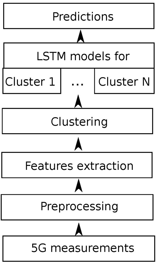
Figure 1. The experiment workflow. We preprocess the captured network traffic and extract its features. To generate the final prediction, we cluster the features and apply LSTM predictive models to each cluster separately.

3.1. Traffic Characteristics

For our prediction, we used two traffic datasets. The first dataset came from a large telecommunication operator, which collected roughly 21 h of traces in Ireland. We divided them into a fixed scenario, where the UE remained in the same position, and a mobile one, where the UE changed its position. A detailed traffic generation and capture methodology is available in [38].

Cellular system operation has diverse characteristics that depend on the specific network deployment details, e.g., antenna heights or cell numbers in an area. Furthermore, the geographical environment also impacts the system. For example, in a city, radio waves are more obstructed by infrastructure than in rural areas. These factors can contribute to unique properties in the collected network traffic. Therefore, we also conducted measurements of a 5G system. For the collection of the network throughput data, we employed G-NetTrack Lite. This is a network monitor and a test tool for mobile networks that runs on a smartphone. To obtain the throughput, we repeatedly downloaded from a server a 1 GB file. The large file allowed the TCP sending window to extend to its maximum size. The network monitor logged the throughput with 1 s granularity. In the case of the mobile scenario, denoted as M2, we drove a car between multiple locations separated by an average distance of 2 km. In each location, we stayed for a random time interval, with an average duration of 5 min. This simulated a typical bus or car drive in an urban area with crossroads, traffic lights, traffic jams, and bus stops. We captured the traffic, and after data cleaning, we had 600 min for a fixed scenario and another 600 min for a mobile one.

Our traces, F2 and M2, had a higher spread between the minimum and maximum values but lower average throughput than the public traces F1 and M1, as shown in Table 2. When examined more closely, both traffic traces had high variability and no clear repeating patterns, as shown in Figure 2. The mobile scenario trace (M2) had slightly higher oscillations and achieved higher throughput as some measurement points were closer to the BS compared to the fixed scenario trace (F2). These high-throughput times were separated by lower-throughput periods where the UE was farther from the BS or was moving. Both traces could be divided into multiple regimes that could be statistically described based on their periods of low and high throughput, as well as periods of low and high variability. The M2 trace exhibited these regimes more clearly, which can be attributed to the switching of the measurement points.

Table 2. Network throughput traces used in the experiments.

Trace	Activity	Length (min)	Average (MB/s)	Min and Max (MB/s)	Source
F1	Fixed	260	5.6	2.7–25	[38]
F2	Fixed	600	5.1	0–37	Author’s measurements
M1	Mobile	459	2.1	0.4–11	[38]
M2	Mobile	600	1.9	0–57	Author’s measurements

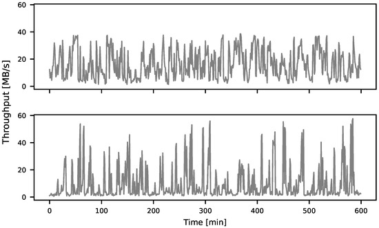
Figure 2. Throughput measured in 5G network. Upper figure—traffic for a fixed UE scenario (F2 trace); Bottom figure—traffic for a mobile UE scenario (M2 trace).

3.2. Feature Extraction

The captured traffic traces required preprocessing before being subjected to the prediction stage. There are many rules regarding preprocessing, but it remains an experiment-intensive art. In our case, the decent amount of data did not mean that the LSTM ANNs provided more accurate prediction. For example, large quantities of data can be relatively similar or correlated, which limits their contribution to ANN learning. As mentioned in Section 3.1, the statistical characteristics of our data changed over time, which is called concept drift. Hence, our task was to identify and group segments of the traces that had similar characteristics to build separate models for them. The individual trace segments could be labelled based on the location of the measurements to facilitate grouping according to additional domain knowledge. However, in reality, there are no such labels, so we propose an automatic mechanism based on feature extraction.

A feature is a lower-dimensional representation mapping

$$\varphi :R^w\to R,\varphi \left(X_{i,w}\right)=\varphi \left([x_{i-w+1},\cdots ,x_i]\right),$$

which captures a specific aspect of the time series $X=\{x_1,x_2,\dots ,x_i,\dots \}$. In our work, we used the mean and variance of $\varphi \left(X_{i,w}\right)$ because they are the primary measures applied in data analysis. The optimal feature selection and number is a complex topic. It depends on the dataset, clustering method, and predictive model. While there are some methods regarding feature selection for a few selected clustering algorithms [39], no such guidelines exist for an ANN ensemble. In other words, the optimal clustering produced by a set of features may not necessarily be the optimal training set for a predictive model. Other examples of features are maximum/minimum, the number of peaks with a certain steepness, their periodicity, or a global trend. For the feature extraction, we used tsfresh [40]. According to the technical documentation, tsfresh provides 63 time series characterization methods and computes a total of 794 time series features.

3.3. Clustering

The purpose of clustering is to group the different segments of network traces based on their implicit similarity. The traces, represented here as time series, can be clustered in many different ways, whose description is beyond the scope of our paper. The most intuitive approach is to compare the whole time series. The series is divided into overlapping segments, which are represented as vectors. Then, each pair of vectors is compared using a distance measure, see Figure 3a. However, defining a suitable measure for distance between unprocessed time series can be a difficult task. The definition must take into account various factors such as high-dimensional space, noise, varying series lengths, different dynamics, and different scales. Therefore, it is recommended to use a clustering algorithm for an interpretable, extracted feature vector; see Figure 3b. Feature-based clustering techniques employ a set of global features that summarize the transient characteristics of time series. This approach is more resilient to noisy data and easier to interpret [41]. We apply the features identified in Section 3.2, namely the mean and variance. Clustering should present less computational burden than a single, more complicated model for the whole trace.

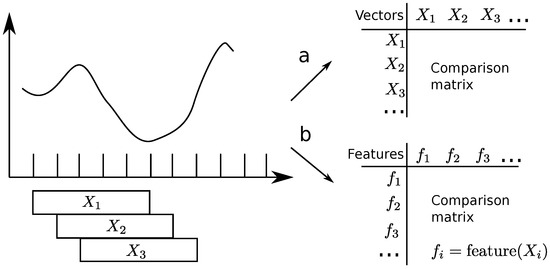
Figure 3. Finding similarities in a univariate time series. Consecutive sliding windows are represented as the vectors $\{X_1,X_2,\dots ,X_n\}$. The vectors are compared (a) directly and (b) through the computed vectors’ features.

Besides the similarity metrics, the clustering method also affects the result [33]. Hence, we employed three algorithms, namely KMeans, OPTICS, and AutoClass. These algorithms represent different clustering approaches. KMeans is a partition-based algorithm, OPTICS is density-based, and AutoClass is probabilistic. The complexity of the algorithms is similar, increasing the chances of obtaining an independent final prediction and making the experiment easier to reproduce. With this selection, we aimed to compare the algorithms’ classes instead of the algorithms themselves.

KMeans is a popular partition-based algorithm, where each data point is assigned to a single cluster. The algorithm defines k centroids, one for each cluster. Then, the centroids absorb nearby data points by applying a specified distance measure. In this process, every point in a dataset is assigned to the centroid closest to it. When all the points have been assigned, the algorithm calculates k new centroids by taking into account the points that were assigned to them. Once it has found the new centroids, it will reassign all the points to the centroid closest to them. This process is repeated until the centroids no longer move significantly.

Figure 4 shows a fragment of the F2 trace with highlighted segments possessing similar statistical characteristics measured by the mean and variance. The segments were selected from a cluster identified by KMeans. The segments have low throughput and variability compared to the rest of the trace.

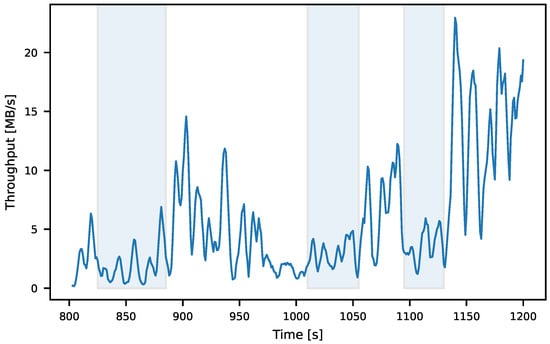
Figure 4. KMeans algorithm applied to the F2 trace. The traffic in the highlighted areas possesses similar statistical characteristics measured by the mean and variance.

Figure 5 presents feature clusters identified by KMeans and extracted from a fragment of the M2 trace. The x-coordinates represent the mean feature, while the y-coordinates represent the variance feature. The groupings have a Y shape. The clusters labelled 1–3 depict traffic fluctuations of different amplitudes—from the smallest ones in cluster 1 to the medium ones in cluster 3. Clusters 4 and 5 describe major increases or drops in the throughput with a non-zero mean change and high variance.

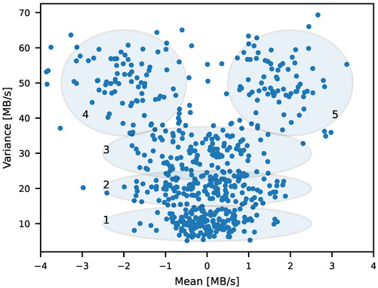
Figure 5. Exemplary two-dimensional clusters for mean and variance features extracted from a fragment of the differenced M2 trace using KMeans algorithm. The clusters labelled 1–3 group traffic fluctuations of different amplitudes. Clusters 4 and 5 describe more significant changes in the network throughput.

The OPTICS algorithm identifies clusters as dense areas separated by less dense ones. Density-based algorithms can discover clusters with arbitrary shapes—an advantage over partition-based algorithms such as KMeans, which can only identify sphere-shaped clusters. OPTICS is based on the same concept as DBSCAN [42], but it overcomes one of DBSCAN’s weaknesses—the inability to identify meaningful data clusters with varying densities. This is particularly relevant in network trace clustering because, as illustrated in Figure 5, the density of data points varies among distinct clusters. To handle this problem, OPTICS uses a reachability distance in addition to the core distance used in DBSCAN. These distances depend on two input parameters: $ϵ$, the distance around an object that constitutes its $ϵ$-neighbourhood, and minPts, a minimum number of points defining the $ϵ$-neighbourhood.

Deterministic clustering methods, such as KMeans and OPTICS, are standard tools for finding groups in data. However, they lack the quantification of uncertainty in the estimated clusters. AutoClass is a clustering algorithm based on the probabilistic model that assigns instances to classes probabilistically. AutoClass is based on a mixture of models and assumes that all the data points are generated from a mixture of a finite number of probability distributions with unknown parameters. The mixture of models can be compared to the generalization of KMeans clustering to incorporate information about the covariance of the data. To build the probabilistic model, the AutoClass algorithm automatically determines the distribution parameters and the number of clusters.

3.4. Long Short-Term Memory Networks

Artificial neural networks (ANNs) are a popular machine learning technique due to their ability to learn complex non-linear relationships between multiple variables, making them accurate and versatile. They can serve as universal function approximators, allowing them to learn and solve complex problems. Initially, single-layered ANNs were more popular than deep ANNs due to training difficulties. However, deep ANNs overcame these issues and gradually replaced single-layered ANNs as a solution to more complex problems. Deep ANNs added more complexity and non-linearity to network traffic models, making them useful for time series prediction, including network traffic. As a result, ANNs have become a universal tool for predicting time series data in various fields.

However, most ANNs have a feed-forward architecture that does not store a trace of previous inputs. They process every input independently and do not memorize information, which is sufficient in many areas, such as computer vision. Nevertheless, as they process the whole input sequence at once, they miss the temporal dependency present in the time series. Hence, Recurrent Neural Networks (RNNs) are better suited for processing time series data. Contrary to feed-forward ANNs, RNNs’ connections form an internal loop. Such an architecture allows one to treat sequences by iterating through their elements and to store information about previously processed data. Training Recurrent Neural Networks (RNNs) with a vanilla recurrent unit can be inefficient due to the vanishing gradient problem, which hinders the ability to retain data from earlier computations. This is because RNNs miss information about long-memory dependencies. However, an advanced type of RNN called a Long Short-Term Memory (LSTM) ANN can overcome this shortcoming. LSTMs allow for long-term memory storage in cells with self-connections, which helps to retain information from earlier computations. LSTM has multiplicative gates in each cell. These gates—the input, output, and forget gates—control information flow and can learn to open and close as needed; see Figure 6. This allows memory cells to store data over long periods of time, making them particularly useful in time series prediction with long temporal dependency. Multiple memory blocks form a hidden layer, and an LSTM model typically consists of an input layer, at least one hidden layer, and an output layer. Deep LSTM architectures with multiple hidden layers can create increasingly higher levels of data representations due to their greater capacity. In this architecture, multiple hidden layers are stacked in such a way that the subsequent layer takes the output of the previous LSTM layer as its input; see Figure 7. In this work, we applied such a multilayer architecture.

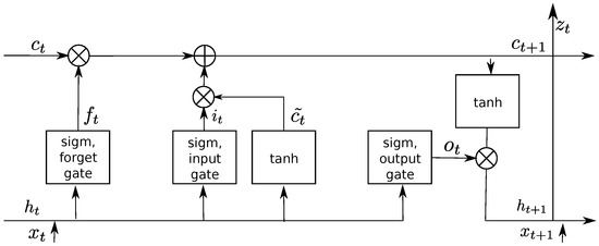
Figure 6. Structure of LSTM memory block: $x_t$ is an input signal at the time t; $c_t$ and $c_{t+1}$ denote cell states at the actual t and future $t+1$ times, respectively; $h_t$ and $h_{t+1}$ are output signals of the cell at t and $t+1$ times, respectively; and b denotes the bias. The symbol + denotes the summation and × the multiplication of signals. The signals $x_t$ and $h_t$ follow the same path but do not interact when entering the cell. The cell output $z_t$ equals the state signal $h_{t+1}$.

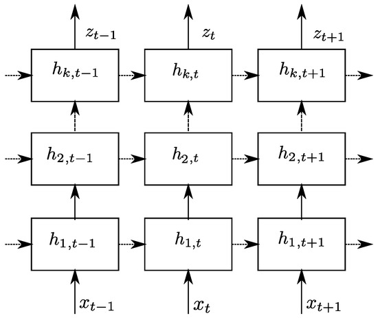
Figure 7. Multilayer LSTM. Hidden layers are stacked in such a way that the output of an LSTM hidden layer is provided to the subsequent LSTM hidden layer.

3.5. Prediction Accuracy

Network traffic prediction in the next time step depends on the historical traffic volumes. Having measurements of the past throughput $\{r_{t-1},\dots ,r_{t-n}\}$, we aim to predict the value of $r_t$. Hence, we use a predictor ${\widehat{r}}_t$, which takes the past throughput

$${\widehat{r}}_t=\varphi (r_{t-1},\dots ,r_{t-n}).$$

(1)

The problem is to determine $\varphi$, which minimizes the difference between ${\widehat{r}}_t$ and $r_t$. To quantify the difference, we opted for the Normalised Root Mean Square Error (NRMSE) as our metric:

$$\begin{array}{c}\hfill \mathrm{NRMSE}\end{array}=\frac{1}{\overline{r}}\sqrt{\frac{{\sum }_{t=1}^N{(r_t-\widehat{r_t})}^2}{N}},$$

(2)

The NRMSE is the squared difference between predictions ${\widehat{r}}_t$ and measured values $r_t$ divided by the number of measurements N. The NRMSE value is an indicator of how well a model fits empirical data. The lower the NRMSE value, the more accurate the prediction. To allow for a comparison of the results across traces with different throughput levels, we normalized the results by an average of observed values $\overline{r}$.

4. Experiment and Results

4.1. Parameters

Table 3 shows the prediction models applied to the network traces. The first model, LSTM, operated on traces without clustering. As the statistical characteristics of the traces listed in Table 2 are too diverse to be described by a single model, we trained the LSTM model separately on each trace (F1, F2, M1, and M2).

Table 3. Summary of the methods used in the experiments.

Method	Clusters				Description
	F1	F2	M1	M2
Universal LSTM	-				Applied for every trace (F1, F2, M1, M2) separately
LSTM + KMeans	4	4	4	5	Clusters a trace then applies the predictive model
LSTM + OPTICS	4	4	5	5
LSTM + AutoClass	3	3	4	4
MA(1)	-				Benchmark predictor $x_t=x_{t-1}+ϵ$

The next three listed models, LSTM + KMeans, LSTM + OPTICS, and LSTM + AutoClass, applied LSTM to the traces clustered by the respective methods. The LSTM networks had two hidden layers compared to three layers for the universal LSTM model—we wanted to replace a single complex model with an ensemble of simpler ones. The models operated on three to five clusters depending on the employed clustering algorithm and the trace. To specify the optimal number of clusters, we employed the Silhouette index (SIL). The SIL measures the distance between feature vectors and the cluster’s centroid compared to the other clusters’ centroids. Its values range from −1 to 1. The closer the SIL value to +1, the better the clustering. Unlike KMeans, OPTICS allows for specifying indirectly the number of clusters by manipulating their input parameters, namely $ϵ$-neighbourhood and minPts. AutoClass, as the name suggests, automatically adjusts the number of clusters to the data.

The last model—MA(1) (a moving average)—represents a naive estimator $x_t=x_{t-1}+ϵ$, where $ϵ$ is white noise. We used the benchmark to check if the complex model could beat the simplest one.

While training the ANNs, we applied K-fold cross-validation. First, we divided our dataset into K equal-sized parts $\{p_1,p_2,\dots ,p_K\}$. Next, we kept one of the parts as the validation set and combined the remaining $K-1$ parts to form the training set. We repeated this process K times, each time leaving another one of the parts out, until we had K different training sets and K different validation sets. For every set, we calculated the NRMSE (2), obtaining its range for every trace. The training parameters for the employed ANNs are listed in Table 4.

Table 4. Values of LSTMs’ selected parameters.

Parameter	Universal LSTM	LSTM + Clustering
Input size	16	16
Batch size	4	4
LSTM hidden states	48	32
LSTM hidden layers	3	2
Initial learning rate	0.001
Optimization algorithm	Adam
Loss function	MAE

4.2. Results

In Figure 8, we present a fragment of the F2 trace, which helps to visualize the traffic characteristics and prediction accuracy. The prediction generally followed the traffic pattern, but sometimes, it overestimated the scope of oscillations in absolute values, particularly in fragments where traffic fluctuations had a higher frequency. Similar to Figure 4, the trace had an irregular structure with no identifiable patterns, which made the prediction difficult. However, there were some periods, such as between 230 s and 300 s, where the trace had more regular oscillations, aiding in clustering and giving the ANNs an edge in prediction.

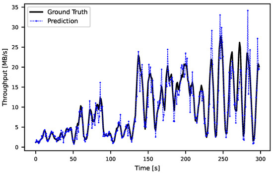
Figure 8. One-step prediction for the F2 trace. The prediction tended to underestimate and overestimate the traffic, especially when its oscillations had a higher amplitude.

Figure 9 shows the distribution of prediction errors for the LSTM, LSTM + KMeans, and MA(1) models using the M2 trace. The histogram for MA(1) is wider, indicating that the errors were higher than in the LSTM-based models. The difference between LSTM and the clustered approach was more subtle but still visible.

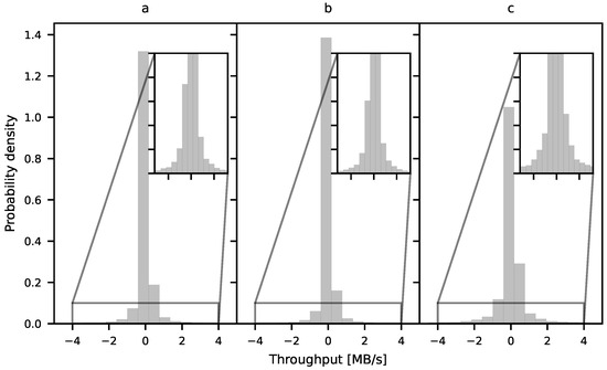
Figure 9. Comparison of prediction error distribution by (a) LSTM, (b) LSTM + KMeans, and (c) MA(1) for the M2 trace. The narrower the histogram, the better the prediction accuracy.

The results presented in Figure 10 and Figure 11 reveal that the clustering approach achieved the lowest NRMSE in both fixed and mobile scenarios. Both the F1 and F2 traces showed similar performance results for the fixed scenario, as illustrated in Figure 10. The error achieved by the LSTM model trained on the whole continuous traces was moderately higher than that of the specialized LSTM models. The MA(1) error was the highest. The results were similar regardless of the applied clustering algorithms. However, a closer examination of the results showed that KMeans obtained a slightly worse score than the remaining two groupings.

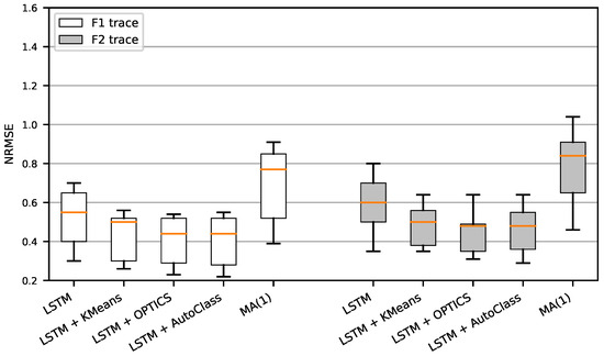
Figure 10. NRMSE of different prediction models for a fixed UE device generating F1 and F2 traces.

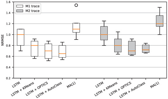
Figure 11. NRMSE of different prediction models for a mobile UE device generating M1 and M2 traces.

In the case of the mobile scenario, shown in Figure 10, the NRMSE was higher for all the models compared to the fixed scenario. Additionally, the universal LSTM model’s error was significantly higher than that of the cluster-based model.

4.3. Discussion

The results show that the ensemble of LSTM ANNs could improve prediction accuracy, especially for traffic generated by a mobile UE device. This finding can be explained in two ways: either the clustering was better, or the clustered data provided to the LSTM model was easier to predict. When considering the former case, the reason for better clustering may have its roots in the mobility pattern of the M1 and M2 traces. In the case of the M2 trace, the UE moved between several places, creating a closed trajectory, which was repeated multiple times. This mobility pattern probably introduced a certain amount of regularity into the trace. The clustering algorithms captured these recurring patterns; however, the same patterns negatively impacted the training of the universal LSTM and MA(1) models. Considering the latter case, some fragments of the UE’s movement path may have had a better quality signal (measured as CQI), which resulted in stable and more predictable throughput. Thus, some models may have achieved significantly better prediction accuracy, and, consequently, they lowered the NRMSE for the whole ensemble. In such a situation, the universal model would also have an adaptation problem when switching repeatedly between relatively stable and irregular trace parts. Unlike in the fixed scenario, the clustering algorithms impacted the result. For both M1 and M2 traces, AutoClass achieved the lowest NRMSE, followed by OPTICS and KMeans. A possible reason for this could be that the clusters generated in the mobile scenario were more specific than those generated in the fixed scenario. With the more diverse groupings, the performance differences among the clustering methods were more visible, and more elaborate algorithms achieved better scores.

Although the prior clustering improved the prediction, the error for the traces generated by a mobile UE device was higher than for the traces from a fixed UE device. This means that the proposed solution could not transform a complex traffic trace into several groups containing simpler traces. After all, the mobile scenario was not a concatenation of multiple fixed scenarios but contained time segments where the UE was on the move. The methods applied, namely feature extraction, clustering, and the LSTM ensemble, were sufficient to give a better result than a single LSTM network. Each of these methods requires more tuning to work optimally, but they should also cooperate with the remaining elements of the prediction workflow. Thus, our work leaves several open questions.

Firstly, which features should be selected to obtain the best clustering? Although feature extraction methods are generic, extracted features often depend on the application context. This means that one set of features that is significant for one time series may not be important to another. The discovery of patterns in data is rarely a one-shot action but rather a process of finding clues, interpreting the results, transforming or augmenting the data, and repeating the cycle. Therefore, another feature selection step is sometimes needed to limit the number of feature dimensions. Although the importance of the selection can be determined using built-in features of the tsfresh algorithm or principal component analysis, these most important features do not necessarily guarantee the best clustering results.

Secondly, what is the optimal number of clusters to divide the traces and result in the best LSTM performance? There are many measures of clustering performance, but do their results translate automatically into a better ensemble of models? Therefore, it might be worth exploring the algorithms that utilize time series information in more detail.

Thirdly, what would be the benefit of localized prediction in the case of more sophisticated prediction models? The effectiveness of prediction models depends on their capacity to match the complexity of the task at hand and the amount of training data they are given. During training, will more complex models with higher capacities memorize the properties of the clustered traces and overfit, leading to poor performance on test data?

Lastly, how much does the prediction depend on the network trace used? In the case of the fixed UE scenario, the results were similar, but in the case of mobile UE devices, there were differences in prediction accuracy. It would be interesting to find the contributory features influencing these results—whether it be a mobility pattern; particular attributes of the environment (e.g., antennas, location, landforms); or a particular UE model used for the measurements.

Though we used the NRMSE (2), a comparison with other research results was almost impossible because other authors have used different measures for prediction accuracy, namely the MSE (Mean Squared Error), RMSE (Root MSE), or MAPE (Mean Absolute Percentage Error). Some of these metrics, like the MSE or RMSE, are not normalized, and the NRMSE is defined differently [11] and cannot be compared. It is worth noting that NRMSE values can vary greatly between different studies. For instance, in [7], the NRMSE ranged from approximately 0.1 to 5.5, depending on the dataset and LSTM ANN, while in [13], the NRMSE was consistently below 0.1 across all experiments. Comparing the results with our previous study [3], our approach obtained a slightly lower NRMSE than the universal model based on bi-directional LSTM. Bi-directional LSTM, which considers additional backward dependencies in data, is a more advanced version of an LSTM ANN.

The obtained results fit the needs of DASH systems. The relatively long video sessions are susceptible to concept drift affecting network traffic. Environmental circumstances like UE number fluctuation within a cell or UE location change are likely to periodically impact the video trace characteristics. Replacing a single predictive model with several simpler models facilitates adaptation to the video player’s streaming algorithm. Aside from DASH systems, the presented results have several potential applications involving short-term traffic prediction, such as network adaptive services; surveillance (e.g., traffic anomaly detection); and 5G network optimization. However, the proposed solution’s implementation in production systems would present a trade-off between accuracy and the computational resources needed to train an ensemble of deep learning models.

5. Conclusions

Large datasets can enhance ANN training but negatively impact the prediction accuracy of global models due to statistical diversity. On the other hand, large datasets are statistically more diverse, which negatively impacts the prediction accuracy of a global model trained on the whole trace. Hence, we clustered the network traces and grouped them according to similar statistical features measured by the mean and variance. For comparison purposes, we applied three clustering techniques, namely KMeans, OPTICS, and AutoClass. For our analysis, we used four traces—two generated in an experiment, and two from a public repository. These traces were collected from fixed and mobile UE devices. To compare the groupings, we used three clustering techniques, namely KMeans, OPTICS, and AutoClass, to assess the robustness of our framework. The experiment’s results showed that prior traces clustering into more statically homogeneous improved the prediction accuracy. The local models—LSTM with different cluster variants—performed better than the global baseline LSTM model, especially in the case of a mobile scenario. All the ANN-based models, whether local or global, achieved significantly better scores than the benchmark model MA(1), where the predictor was the time series’ previous value. In the case of traces produced by stationary UE devices, the local models yielded comparable outcomes. However, for the mobile scenario, the more advanced clustering techniques like AutoClass and OPTICS showed a lower prediction error. A possible explanation for these results may be that the traces generated in the mobile environment were more susceptible to clustering and generated more specific groups, which were easier to capture by more elaborate clustering algorithms. Overall, the results showed that the multiple local models working on clustered data effectively exploited the similarities of the network traces and consequently outperformed the single model approach. The proposed algorithm can be used primarily in adaptive video streaming to improve the selection of a video’s bitrate. The predictive models can be integrated into the client’s bitrate selection logic, replacing the default decision mechanism based on the moving average of historical bit rates.

References

- Yuan, X.; Wu, M.; Wang, Z.; Zhu, Y.; Ma, M.; Guo, J.; Zhang, Z.L.; Zhu, W. Understanding 5G performance for real-world services: A content provider’s perspective. In Proceedings of the ACM SIGCOMM 2022 Conference, Amsterdam, The Netherlands, 22–26 August 2022; pp. 101–113. [Google Scholar]
- Yang, X.; Lin, H.; Li, Z.; Qian, F.; Li, X.; He, Z.; Wu, X.; Wang, X.; Liu, Y.; Liao, Z.; et al. Mobile access bandwidth in practice: Measurement, analysis, and implications. In Proceedings of the ACM SIGCOMM 2022 Conference, Amsterdam, The Netherlands, 22–26 August 2022; pp. 114–128. [Google Scholar]
- Biernacki, A. Improving streaming video with deep learning-based network throughput prediction. Appl. Sci. 2022, 12, 10274. [Google Scholar] [CrossRef]
- Famaey, J.; Latré, S.; Bouten, N.; Van de Meerssche, W.; De Vleeschauwer, B.; Van Leekwijck, W.; De Turck, F. On the merits of SVC-based HTTP adaptive streaming. In Proceedings of the 2013 IFIP/IEEE International Symposium on Integrated Network Management (IM 2013), Ghent, Belgium, 27–31 May 2013; pp. 419–426. [Google Scholar]
- Li, F.; Chen, W.; Shui, Y. Analysis of non-stationarity for 5.9 GHz channel in multiple vehicle-to-vehicle scenarios. Sensors 2021, 21, 3626. [Google Scholar] [CrossRef]
- Liu, J.; Nazeri, A.; Zhao, C.; Abuhdima, E.; Comert, G.; Huang, C.T.; Pisu, P. Investigation of 5G and 4G V2V Communication Channel Performance Under Severe Weather. In Proceedings of the 2022 IEEE International Conference on Wireless for Space and Extreme Environments (WiSEE), Winnipeg, MB, Canada, 12–14 October 2022; pp. 12–17. [Google Scholar] [CrossRef]
- He, Q.; Moayyedi, A.; Dan, G.; Koudouridis, G.P.; Tengkvist, P. A Meta-Learning Scheme for Adaptive Short-Term Network Traffic Prediction. IEEE J. Sel. Areas Commun. 2020, 38, 2271–2283. [Google Scholar] [CrossRef]
- Makridakis, S.; Spiliotis, E.; Assimakopoulos, V. Statistical and Machine Learning forecasting methods: Concerns and ways forward. PLoS ONE 2018, 13, e0194889. [Google Scholar] [CrossRef] [PubMed]
- Lohrasbinasab, I.; Shahraki, A.; Taherkordi, A.; Delia Jurcut, A. From statistical- to machine learning-based network traffic prediction. Trans. Emerg. Telecommun. Technol. 2022, 33, e4394. [Google Scholar] [CrossRef]
- Santos Escriche, E.; Vassaki, S.; Peters, G. A comparative study of cellular traffic prediction mechanisms. Wirel. Netw. 2023, 29, 2371–2389. [Google Scholar] [CrossRef]
- Na, H.; Shin, Y.; Lee, D.; Lee, J. LSTM-based throughput prediction for LTE networks. ICT Express 2023, 9, 247–252. [Google Scholar] [CrossRef]
- Kim, M. Network traffic prediction based on INGARCH model. Wirel. Netw. 2020, 26, 6189–6202. [Google Scholar] [CrossRef]
- Trinh, H.D.; Giupponi, L.; Dini, P. Mobile traffic prediction from raw data using LSTM networks. In Proceedings of the 2018 IEEE 29th Annual International Symposium on Personal, Indoor and Mobile Radio Communications (PIMRC), Bologna, Italy, 9–12 September 2018; pp. 1827–1832. [Google Scholar]
- Minovski, D.; Ogren, N.; Ahlund, C.; Mitra, K. Throughput Prediction using Machine Learning in LTE and 5G Networks. IEEE Trans. Mob. Comput. 2021, 22, 1825–1840. [Google Scholar] [CrossRef]
- Labonne, M.; López, J.; Poletti, C.; Munier, J.B. Short-Term Flow-Based Bandwidth Forecasting using Machine Learning. arXiv 2020, arXiv:2011.14421. [Google Scholar]
- Lin, C.Y.; Su, H.T.; Tung, S.L.; Hsu, W.H. Multivariate and propagation graph attention network for spatial-temporal prediction with outdoor cellular traffic. In Proceedings of the 30th ACM International Conference on Information & Knowledge Management, Virtual Event, 1–5 November 2021; pp. 3248–3252. [Google Scholar]
- Zhao, N.; Wu, A.; Pei, Y.; Liang, Y.C.; Niyato, D. Spatial-temporal aggregation graph convolution network for efficient mobile cellular traffic prediction. IEEE Commun. Lett. 2021, 26, 587–591. [Google Scholar] [CrossRef]
- Qiu, C.; Zhang, Y.; Feng, Z.; Zhang, P.; Cui, S. Spatio-Temporal Wireless Traffic Prediction With Recurrent Neural Network. IEEE Wirel. Commun. Lett. 2018, 7, 554–557. [Google Scholar] [CrossRef]
- Wei, B.; Kawakami, W.; Kanai, K.; Katto, J.; Wang, S. TRUST: A TCP throughput prediction method in mobile networks. In Proceedings of the 2018 IEEE Global Communications Conference (GLOBECOM), Abu Dhabi, United Arab Emirates, 9–13 December 2018; pp. 1–6. [Google Scholar]
- Zhohov, R.; Palaios, A.; Geuer, P. One Step Further: Tunable and Explainable Throughput Prediction based on Large-scale Commercial Networks. In Proceedings of the 2021 IEEE 4th 5G World Forum (5GWF), Montreal, QC, Canada, 13–15 October 2021; pp. 430–435. [Google Scholar] [CrossRef]
- Narayanan, A.; Ramadan, E.; Mehta, R.; Hu, X.; Liu, Q.; Fezeu, R.A.; Dayalan, U.K.; Verma, S.; Ji, P.; Li, T.; et al. Lumos5G: Mapping and predicting commercial mmWave 5G throughput. In Proceedings of the ACM Internet Measurement Conference, Virtual Event, 27–29 October 2020; pp. 176–193. [Google Scholar]
- Sliwa, B.; Falkenberg, R.; Wietfeld, C. Towards cooperative data rate prediction for future mobile and vehicular 6G networks. In Proceedings of the 2020 2nd 6G Wireless Summit (6G SUMMIT), Levi, Finland, 17–20 March 2020; pp. 1–5. [Google Scholar]
- Yue, C.; Jin, R.; Suh, K.; Qin, Y.; Wang, B.; Wei, W. LinkForecast: Cellular Link Bandwidth Prediction in LTE Networks. IEEE Trans. Mob. Comput. 2018, 17, 1582–1594. [Google Scholar] [CrossRef]
- Lee, H.; Kang, Y.; Gwak, M.; An, D. Bi-LSTM model with time distribution for bandwidth prediction in mobile networks. ETRI J. 2023, 1–13. [Google Scholar] [CrossRef]
- Raca, D.; Zahran, A.H.; Sreenan, C.J.; Sinha, R.K.; Halepovic, E.; Jana, R.; Gopalakrishnan, V. On Leveraging Machine and Deep Learning for Throughput Prediction in Cellular Networks: Design, Performance, and Challenges. IEEE Commun. Mag. 2020, 58, 11–17. [Google Scholar] [CrossRef]
- Li, Y.; Ma, Z.; Pan, Z.; Liu, N.; You, X. Prophet model and Gaussian process regression based user traffic prediction in wireless networks. Sci. China Inf. Sci. 2020, 63, 142301. [Google Scholar] [CrossRef]
- Liu, C.; Wu, T.; Li, Z.; Wang, B. Individual traffic prediction in cellular networks based on tensor completion. Int. J. Commun. Syst. 2021, 34, e4952. [Google Scholar] [CrossRef]
- Wang, W.; Zhou, C.; He, H.; Wu, W.; Zhuang, W.; Shen, X. Cellular traffic load prediction with LSTM and Gaussian process regression. In Proceedings of the ICC 2020—2020 IEEE International Conference on Communications (ICC), Dublin, Ireland, 7–11 June 2020; pp. 1–6. [Google Scholar]
- Xing, X.; Lin, Y.; Gao, H.; Lu, Y. Wireless Traffic Prediction with Series Fluctuation Pattern Clustering. In Proceedings of the 2021 IEEE International Conference on Communications Workshops (ICC Workshops), Montreal, QC, Canada, 14–23 June 2021; pp. 1–6. [Google Scholar] [CrossRef]
- Mahdy, B.; Abbas, H.; Hassanein, H.; Noureldin, A.; Abou-zeid, H. A Clustering-Driven Approach to Predict the Traffic Load of Mobile Networks for the Analysis of Base Stations Deployment. J. Sens. Actuator Netw. 2020, 9, 53. [Google Scholar] [CrossRef]
- Shawel, B.S.; Mare, E.; Debella, T.T.; Pollin, S.; Woldegebreal, D.H. A Multivariate Approach for Spatiotemporal Mobile Data Traffic Prediction. Eng. Proc. 2022, 18, 10. [Google Scholar] [CrossRef]
- Schmid, J.; Schneider, M.; Höß, A.; Schuller, B. A comparison of AI-based throughput prediction for cellular vehicle-to-server communication. In Proceedings of the 2019 15th International Wireless Communications & Mobile Computing Conference (IWCMC), Tangier, Morocco, 24–28 June 2019; pp. 471–476. [Google Scholar]
- Jiang, W. Cellular traffic prediction with machine learning: A survey. Expert Syst. Appl. 2022, 201, 117163. [Google Scholar] [CrossRef]
- Bayram, F.; Ahmed, B.S.; Kassler, A. From concept drift to model degradation: An overview on performance-aware drift detectors. Knowl.-Based Syst. 2022, 245, 108632. [Google Scholar] [CrossRef]
- Agrahari, S.; Singh, A.K. Concept Drift Detection in Data Stream Mining: A literature review. J. King Saud Univ.-Comput. Inf. Sci. 2022, 34, 9523–9540. [Google Scholar] [CrossRef]
- Ge, J.; Li, T.; Wu, Y. Concept Drift Detection for Network Traffic Classification. In AI and Machine Learning for Network and Security Management; IEEE: Piscataway, NJ, USA, 2023; pp. 91–108. [Google Scholar] [CrossRef]
- Liu, Z.; Godahewa, R.; Bandara, K.; Bergmeir, C. Handling Concept Drift in Global Time Series Forecasting. In Forecasting with Artificial Intelligence: Theory and Applications; Hamoudia, M., Makridakis, S., Spiliotis, E., Eds.; Springer: Cham, Switzerland, 2023; pp. 163–189. [Google Scholar] [CrossRef]
- Raca, D.; Leahy, D.; Sreenan, C.J.; Quinlan, J.J. Beyond throughput, the next generation: A 5G dataset with channel and context metrics. In Proceedings of the 11th ACM Multimedia Systems Conference, Istanbul, Turkey, 8–11 June 2020; pp. 303–308. [Google Scholar] [CrossRef]
- Hancer, E.; Xue, B.; Zhang, M. A survey on feature selection approaches for clustering. Artif. Intell. Rev. 2020, 53, 4519–4545. [Google Scholar] [CrossRef]
- Christ, M.; Braun, N.; Neuffer, J.; Kempa-Liehr, A.W. Time Series FeatuRe Extraction on basis of Scalable Hypothesis tests (tsfresh—A Python package). Neurocomputing 2018, 307, 72–77. [Google Scholar] [CrossRef]
- Fulcher, B.D. Feature-based time-series analysis. In Feature Engineering for Machine Learning and Data Analytics; CRC Press: Boca Raton, FL, USA, 2018; pp. 87–116. [Google Scholar]
- Schubert, E.; Sander, J.; Ester, M.; Kriegel, H.P.; Xu, X. DBSCAN revisited, revisited: Why and how you should (still) use DBSCAN. ACM Trans. Database Syst. (TODS) 2017, 42, 1–21. [Google Scholar] [CrossRef]
Disclaimer/Publisher’s Note: The statements, opinions and data contained in all publications are solely those of the individual author(s) and contributor(s) and not of MDPI and/or the editor(s). MDPI and/or the editor(s) disclaim responsibility for any injury to people or property resulting from any ideas, methods, instructions or products referred to in the content. |
© 2024 by the author. Licensee MDPI, Basel, Switzerland. This article is an open access article distributed under the terms and conditions of the Creative Commons Attribution (CC BY) license (https://creativecommons.org/licenses/by/4.0/).