On Weighted Sum Rate of Multi-User Photon-Counting Multiple-Input Multiple-Output Visible Light Communication Systems under Poisson Shot Noise

Abstract

Photon counting has been proven to possess excellent signal detection capabilities at low power levels and has extensive potential applications in sixth-generation (6G) communications. However, the inherent dependency between the signal and noise complicates system analysis, and optimizing achievable rates in photon-counting visible light communication (VLC) systems remains unresolved. This paper introduces a new method aimed at minimizing multi-user interference (MUI) through a zero-forcing (ZF) scheme and maximizing the weighted sum rate of the proposed downlink multi-user photon-counting multiple-input multiple-output (MU-PhC-MIMO) VLC system by solving an optimization problem. The key point lies in our utilization of the ZF approach to derive a reasonable asymptotic approximation expression for the weighted sum rate. Subsequently, we use variable substitution and methods like successive convex approximation (SCA) to iteratively convexify the non-convex optimization problem and maximize the weighted sum rate under the ZF form. Compared to other algorithms, this approach can save 2.5 dB of transmission power to achieve the same system-weighted sum rate and significantly outperforms the repetition coding scheme at sufficient transmission power.

1. Introduction

Visible light communication (VLC) serves as a beneficial complement to radio frequency (RF) communication [1], offering the potential to address the scarcity of spectrum resources in RF communication and thereby alleviate pressure on wireless communication networks. Recently, VLC has gained immense traction because of its low cost, low power consumption, and license-free indoor applications in the context of sixth-generation (6G) communication systems [2]. In VLC systems, indoor wireless data are transferred over the optical spectrum using intensity modulation/direct detection (IM/DD) [3]. Light-emitting diodes (LEDs) serve dual purposes for both lighting and data transmission, while photodetectors (PDs) are used to detect the transmitted data [4]. Currently, to enhance the performance of indoor communication systems, numerous LEDs and PDs are deployed within indoor environments, forming multiple-input multiple-output (MIMO) VLC systems.

Photon-counting technology exhibits excellent capabilities in detecting optical signals. When the communication system operates at low power [5], particularly in power-constrained IoT applications, this advantage becomes even more prominent. In such scenarios, traditional optical communication receivers struggle to operate effectively in the presence of extremely weak light. However, the photon-counting receiver utilizes the principle of photon counting and high-sensitivity detectors to achieve reliable optical signal reception and decoding at extremely low optical power levels. We delve into a more microscopic perspective, considering light as being composed of discrete particles called photons. In the traditional field of optical communications, scholars primarily focus on communication system models affected by additive white Gaussian noises (AWGNs). In contrast, photon counting introduces quantum effects due to the discrete nature of light signals, resulting in Poisson shot noises [5], which are signal-dependent. Typically, the photon-counting process can be characterized by two independent parameters [6]—the background radiation and the expected average signal value—and we refer to it as a Poisson counting process (PCP) [5]. This process exhibits non-linear characteristics, posing significant challenges to the analysis and optimization of photon-counting communication systems.

The achievable rate is a critical metric in communication systems, as it directly impacts the efficiency and performance of communication. This metric is equally important and worth researching in photon-counting VLC systems. In MIMO systems, alleviating multi-user interference (MUI) and enhancing achievable rates is typically achieved by using precoding techniques at the transmitter. However, this is not straightforward for photon-counting MIMO VLC systems, as the inherent correlation between the signal and noise in the PCP leads to a fundamental change in the expression of the rate, rendering the classic Shannon formula inapplicable to photon-counting systems. Moreover, this signal-dependent shot noise exhibits non-linear characteristics, posing significant challenges to the analysis and optimization of photon-counting communication systems. This also implies that the mature precoding techniques in MIMO VLC systems in AWGN channels are not applicable in photon-counting systems.

1.1. Related Works

Most research on multi-user VLC systems currently concentrates on mitigating MUI [7]. Various precoding strategies have been devised to achieve specific goals, such as minimizing the maximum mean square error (MSE) [7], maximizing the minimum signal-to-interference-plus-noise ratio (SINR) [8], and optimizing the maximum achievable sum rate of the systems [9].

Currently, the design of precoding schemes in VLC systems predominantly focuses on the linear design part due to its ease of operation [10,11,12,13,14,15,16,17]. Shen et al. [10] introduced a precoding design based on maximizing the rates of multi-user multiple-input single-output (MISO) VLC systems. Subsequently, they expanded this non-alternating method to optimize robust minimum mean square error (MMSE) precoding [11]. According to the characteristics of multi-user scenarios, Máximo et al. [12] proposed the selectivity of the receiving angle for each user. Then, they combined this with a linear zero-forcing (ZF) precoding scheme to further enhance the system’s performance. By capitalizing on LED characteristics and block diagonalization precoding (BDP) technology, Zhao et al. [13] designed a weighted-adjustment block diagonalization precoding (WA-BDP) scheme for multi-user MIMO VLC systems. They further introduced spatial dimming (SD) built on LED selection and proposed an SD-WA-BDP scheme, maximizing LED utilization for simultaneous illumination and communication purposes. Ma et al. [14] investigated the development of linear coordinated precoding strategies to enable coordinated multi-point (CoMP) communication in VLC networks. Sifaou et al. [15] studied the robust joint design of transmission precoders and reception filters for multi-user MIMO VLC systems, aiming to maximize the minimum SINR. Later, Zhao et al. [16] optimized these robust transmission precoders to maximize the sum capacity under worst-case scenarios. Based on the properties of Farey sequences, Wang et al. [17] proposed an optimal precoding scheme designed for multi-user MISO VLC systems, accounting for dual constraints related to illumination and communication.

There has also been extensive research on nonlinear precoding designs [18,19,20]. Compared to linear precoding schemes, nonlinear precoding incurs higher energy consumption and complexity but achieves higher signal-to-noise ratios (SNR). Yu et al. [18] proposed ZF dirty-paper coding to attain the maximum channel capacity in MIMO systems, whereas Kim et al. [19] introduced Tomlinson–Harashima precoding (THP) to reduce complexity. Wang et al. [20] developed a successive interference cancellation (SIC)-based precoding scheme with sub-connected architecture (SIC-SA) to address severe MUI issues in MIMO VLC systems.

In addition to the research on precoding design in IM/DD MISO or MIMO VLC systems, there has been extensive research on multi-carrier VLC systems to achieve improved spectral efficiency [21,22]. Feng et al. [21] proposed a spatial modulation scheme based on ZF and MMSE precoding for indoor MU-MIMO orthogonal frequency-division multiplexing (OFDM) VLC systems using direct current bias. After incorporating their designed transmit antenna selection algorithm, the results demonstrated significant improvements over traditional modulation schemes. Wang et al. [22] focused on each subcarrier of OFDM and used a complex channel matrix in the frequency domain to calculate the corresponding precoding matrix, aiming to eliminate inter-user interference. The results demonstrated the superiority of frequency domain-based precoding algorithms in scenarios with low light power and close user distances.

However, current analyses of MIMO VLC systems mainly rely on AWGN channel models, which are not appropriate for photon-counting VLC systems. This is because the AWGN channel models fail to capture the correlation between the signal and noise. In photon-counting VLC systems, especially in situations where the received signal intensity is weak, this correlation becomes notably significant. Ge et al. [5] proposed an alternating optimization algorithm based on the MMSE criterion for photon-counting MIMO ultraviolet (UV) light systems. This algorithm achieves the joint design of precoders and equalizers. Arya et al. [23] proposed an MMSE receiver to mitigate MUI in a Poisson channel-based multi-user indoor communication system employing UV light. They employed a second-order cone program to create a downlink beamformer.

To the best of our knowledge, there has not yet been a specific analysis regarding the sum rates of multi-user, photon-counting MIMO (MU-PhC-MIMO) VLC systems affected by Poisson shot noises. To address this gap, we examine the weighted sum rate of MU-PhC-MIMO VLC systems in the presence of Poisson shot noises and devise a novel ZF-based precoding algorithm to optimize the weighted sum rate.

1.2. Contributions

We present a novel method to optimize the weighted sum rate of an MU-PhC-MIMO VLC system in the presence of Poisson shot noises. This is accomplished by utilizing a ZF-based approach to mitigate MUI and approximate the system’s weighted sum-rate expression and then using a sequence of convexification processes to iteratively optimize the weighted sum rate of the system based on this approximation. This paper’s primary contributions can be outlined as follows:

• This paper derives the expression for the weighted sum rate of an MU-PhC-MIMO VLC system based on the definition of mutual information. Additionally, it provides an approximate expression for the proposed system’s weighted sum rate under the minimized MUI, which is obtained utilizing a ZF approach.
• We propose a new optimization problem targeting the precoding matrix, aiming to maximize the weighted sum rate of the proposed MU-PhC-MIMO VLC system while minimizing MUI using the aforementioned ZF scheme.
• A novel sub-algorithm is developed to address the updated problem by employing variable substitution and successive convex approximation (SCA). After the analysis, this sub-algorithm is expected to converge to a robust solution that meets the Karush–Kuhn–Tucker (KKT) conditions. Afterward, by utilizing this sub-algorithm to traverse through all feasible scenarios, we can eventually obtain the optimal solution for the entire optimization problem.
• We also introduce a low-complexity alternative algorithm that achieves results close to those of the exhaustive algorithm. However, it significantly reduces discussions about possibilities, thereby reducing the algorithm’s complexity from exponential to polynomial levels.

Extensive simulations illustrate that the proposed algorithms can save the system 2.5 dB of transmit peak power compared to the classic ZF precoding scheme at low transmit power. At high transmit power, the sum rate of our system significantly surpasses that of the repetition coding scheme. Both of the proposed algorithms exhibit nearly identical performance. Furthermore, we show that increased active LEDs and lower DC bias power can further enhance system performance.

The structure of the remainder of this paper is as follows. In Section 2, we introduce the proposed MU-PhC-MIMO VLC system and give the system’s framework. In Section 3, we analyze the weighted sum rate of the MU-PhC-MIMO VLC system and provide an asymptotic approximation of the weighted sum rate based on the ZF scheme. We outline the problem under consideration and describe the proposed algorithms in Section 4. In Section 5, we present the outcomes of our simulations. Finally, we summarize this paper in Section 6.

Notations: $\mathcal{R}$ denotes the set of real numbers; ${\mathcal{R}}_{+}$ denotes the set of positive real numbers; lowercase bold type indicates column vectors; uppercase bold type indicates matrices; ${(·)}^T$ signifies transpose; $|·|$ signifies absolute value; ${\parallel ·\parallel }_p$ signifies the p-norm, where $p=1,2,\cdots ,\infty$; ${log}_2(·)$ represents a logarithm with base 2; $ln(·)$ represents a natural logarithm with base Euler’s number; $Pr(·)$ stands for probability; $Pr(·|·)$ stands for conditional probability; and $Pr(·,·)$ stands for joint probability.

2. System Model and Assumptions

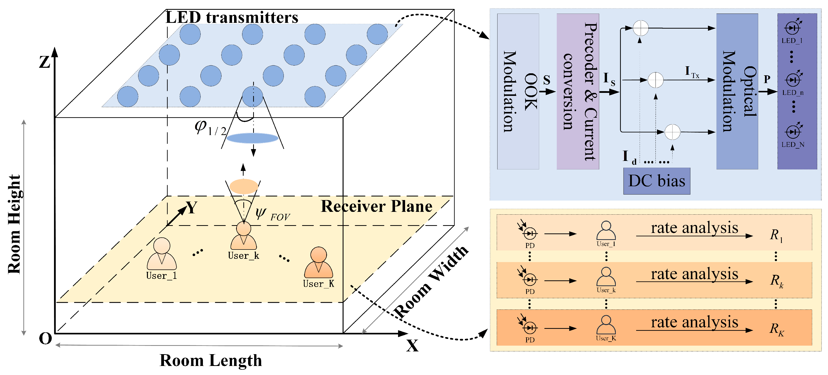
In this paper, we investigate a downlink MU-PhC-MIMO VLC system, the specific block diagram of which is fully described in Figure 1. The transmitting end comprises a device, which has N LED arrays. The entire system caters to K users, each equipped with a single PD. We use the identifier User_k to represent the k-th user, where $k=1,\cdots ,K$.

Figure 1. Schematic diagram of the proposed downlink MU-PhC-MIMO VLC system.

2.1. Transmitter

Due to its ease of implementation and theoretical analysis, on-off keying (OOK) modulation has found widespread application in the domain of optical communication. In our system, we employ OOK modulation to process the raw information and obtain the initial signal for the system. Let $S_k$ denote the modulated data that the transmitter needs to send to User_k, whereas the corresponding $\mathit{S}={\left[S_1,\cdots ,S_K\right]}^T$ denotes the data vector that the transmitter needs to send to all users. We assume that OOK modulation is equiprobable, with $S_k\in \{-1,1\}$ and $Pr(S_k=1)=Pr(S_k=-1)=\frac{1}{2}$. The analysis and algorithms developed in this paper can be easily extended to other modulation methods, such as M-PAM, but require more complex analysis and higher computational complexity.

The symbol $\mathit{S}$ undergoes a linear transformation through a precoding matrix $\mathit{W}\in {\mathcal{R}}^{N\times K}$. The aim is to facilitate collaboration among multiple users, utilizing the same temporal resources for communication tasks and mitigating interference among users to a certain extent. We introduce the constraint ${\parallel \mathit{W}\parallel }_{\infty }\le 1$ for matrix $\mathit{W}$ to ensure that the designed precoding matrix is normalized.

Subsequently, the data are modulated into a current quantity, ${\mathit{I}}_{\mathrm{S}}=\left[I_{S,1},\cdots ,I_{S,N}\right]\in {\mathcal{R}}^{N\times 1}$, without DC bias. ${\mathit{I}}_{\mathrm{S}}$ can be calculated from $\mathit{S}$, $\mathit{W}$, and $\Lambda$, i.e., ${\mathit{I}}_{\mathrm{S}}=\Lambda \mathit{W}\mathit{S}=\Lambda {\sum }_{k=1}^K{\mathit{w}}_k{S}_k$, where $\Lambda \in {\mathcal{R}}_{+}$ represents the parameter for current modulation [24], and ${\mathit{w}}_k$ represents the k-th column of matrix $\mathit{W}$. To ensure that all data within the IM remain non-negative, we need to add DC biases, denoted as ${\mathit{I}}_{\mathrm{d}}={\left[I_{\mathrm{d},1},\cdots ,I_{\mathrm{d},N}\right]}^T\in {\mathcal{R}}^{N\times 1}$, after ${\mathit{I}}_{\mathrm{S}}$. Finally, the emitted current signal ${\mathit{I}}_{\mathrm{Tx}}\in {\mathcal{R}}^{N\times 1}$ can be expressed as:

$${\mathit{I}}_{\mathrm{Tx}}={\mathit{I}}_{\mathrm{S}}+{\mathit{I}}_{\mathrm{d}}=\Lambda \sum _{k=1}^K{\mathit{w}}_k{S}_k+{\mathit{I}}_{\mathrm{d}}.$$

(1)

Ultimately, through optical modulation, we can obtain the transmitted optical signal vector $\mathit{P}\in {\mathcal{R}}^{N\times 1}$, defined as follows:

$$\mathit{P}=U\Lambda \sum _{k=1}^K{\mathit{w}}_k{S}_k+U{\mathit{I}}_{\mathrm{d}}=P_{\mathrm{s}}\sum _{k=1}^K{\mathit{w}}_k{S}_k+U{\mathit{I}}_{\mathrm{d}},$$

(2)

where U represents the voltage parameter, and we define $P_{\mathrm{s}}=U\Lambda$ as the peak transmit power per symbol.

2.2. Channel Model

In the environment of indoor VLC systems, line-of-sight (LOS) links constitute a significant portion of the signal power [25]. For simplicity’s sake, this paper primarily focuses on discussing channel conditions within LOS links. We use ${\mathit{g}}_k\in {\mathcal{R}}^{N\times 1},\forall k$ to denote the channel vector between the LED arrays and User_k, denoted as ${\mathit{g}}_k={\left[g_{1,k},\cdots ,g_{N,k}\right]}^T,\forall k$. The channel gain $g_{i,k}$ from the i-th LED to the k-th user can be obtained using the Lambertian model [26], defined as follows

$$\begin{array}{c}\hfill g_{i,k}=\left\{\begin{array}{cc}\frac{(\kappa +1)A_{\mathrm{r}}}{2\pi l_{i,k}^2}T\left({\psi }_{i,k}\right)G\left({\psi }_{i,k}\right){cos}^{\kappa }\left({\phi }_{i,k}\right)cos\left({\psi }_{i,k}\right),\hfill & \mathrm{if}\left|{\psi }_{i,k}\right|\le {\psi }_{\mathrm{F}\mathrm{o}\mathrm{V}};\hfill \\ 0,\hfill & \mathrm{if}\left|{\psi }_{i,k}\right|>{\psi }_{\mathrm{F}\mathrm{o}\mathrm{V}},\hfill \end{array}\right.\end{array}$$

(3)

where $A_{\mathrm{r}}$ represents the receiving area of the PD; $l_{i,k}$ is the straight-line distance from the i-th LED to User_k; ${\phi }_{i,k}$, ${\psi }_{i,k}$, and ${\psi }_{\mathrm{F}\mathrm{o}\mathrm{V}}$ denote the emission angle starting from the transmitter axis, the reception angle starting from the receiver axis, and the field-of-view (FOV) angle of the PD, respectively; $T\left({\psi }_{i,k}\right)$ refers to the gain of the optical filter; and $\kappa =-\frac{ln2}{ln\left(cos\left({\phi }_{1/2}\right)\right)}$ denotes the Lambertian radiation order, which is determined by the half-irradiance semi-angle ${\phi }_{1/2}$. $G\left({\psi }_{i,k}\right)$ represents the light concentrator’s gain and is denoted by:

$$\begin{array}{c}\hfill G\left({\psi }_{i,k}\right)=\left\{\begin{array}{cc}\frac{o^2}{{sin}^2\left({\psi }_{\mathrm{F}\mathrm{o}\mathrm{V}}\right)},& \mathrm{if}\left|{\psi }_{i,k}\right|\le {\psi }_{\mathrm{F}\mathrm{o}\mathrm{V}};\hfill \\ 0,& \mathrm{if}\left|{\psi }_{i,k}\right|>{\psi }_{\mathrm{F}\mathrm{o}\mathrm{V}},\hfill \end{array}\right.\end{array}$$

(4)

where o is the reflective index.

In this paper, we assume that the transmitter has perfect channel state information (CSI) for all users. This assumption is deemed reasonable in VLC systems, as users’ positions and channel parameters can be reliably obtained. Keskin et al. [27] proposed a receiver localization algorithm to acquire receiver position information. In scenarios where environmental factors such as temperature, atmospheric turbulence, lighting, reflections, shadowing, and other factors impact the communication channel and the background radiation, relying solely on user location information may introduce biases in the CSI. However, both the intensity of background radiation and the channel parameters can be determined through pilot-based measurements or other effective channel estimations. These techniques can help mitigate the effects of environmental factors and provide accurate CSI and the intensity of background radiation. Regarding channel parameter estimation, various algorithms, such as least squares [28], statistical Bayesian MMSE [29], and neural networks [30], can be utilized to estimate channel interference and provide feedback to the transmitter.

2.3. Receiver

Utilizing the photoelectric effect [31], photons detected by a PD can be converted into electrons. We denote $\tau$ as the duration of each symbol. Within a $\tau$ slot, the electron count received by User_k is represented as $Y_k,\forall k$. Given the characteristics of photon counting, this process is a probabilistic measurement process [31] following a Poisson distribution [32]. The conditional probability density function (PDF) of this process is expressed as follows:

$$Pr\left(Y_k=y_k\mid \mathit{S}=\mathit{s}\right)=\frac{{\left({\lambda }_k\right)}^{y_k}}{y_k!}exp\left(-{\lambda }_k\right),$$

(5)

where $y_k=0,1,\cdots ,\infty ,\forall k$ refers to an integer that is non-negative, representing the possible received count, and the vector $\mathit{s}$ denotes the possible realization of $\mathit{S}$, encompassing $2^K$ possibilities. ${\lambda }_k$ represents the average photon count received at User_k, which can be obtained by

$${\lambda }_k=\zeta \frac{{\mathit{g}}_k^T\mathit{P}\tau }{ħv}+n_{\mathrm{b}}=\zeta \frac{{\mathit{g}}_k^T\left(P_{\mathrm{s}}\mathit{W}\mathit{S}+U{\mathit{I}}_{\mathrm{d}}\right)\tau }{ħv}+n_{\mathrm{b}}=\zeta {\mathit{g}}_k^T\left(n_{\mathrm{s}}\mathit{W}\mathit{S}+\mathit{d}\right)+n_{\mathrm{b}}.$$

(6)

where $ħ=6.626\times {10}^{-34}\mathrm{J}·\mathrm{s}$, $\zeta$, and v represent the Planck’s constant, the quantum efficiency of the photon-counting process, and the frequency of visible light, respectively. Let $P_{\mathrm{b}}$ represent the incident background light power, whereas the average photon count generated by background radiation within a single $\tau$ slot is denoted as $n_{\mathrm{b}}=\zeta \frac{P_{\mathrm{b}}\tau }{ħv}$. For ease of expression, we denote the signal strength and bias strength as $n_{\mathrm{s}}=\frac{P_{\mathrm{s}}\tau }{ħv}$ and $\mathit{d}=\frac{U\tau }{ħv}{\mathit{I}}_{\mathrm{d}}$, respectively. Equation (6) is derived by substituting (2).

3. Rate Analysis of MU-PhC-MIMO VLC Systems

This section starts by analyzing the achievable rate for ${\mathrm{User}}_k,\forall k$, deriving the corresponding expression, and providing the expression for the weighted sum rate under the scenario of K users. Additionally, we discuss an approximate expression for system rates based on the ZF scheme.

3.1. Achievable Weighted Sum Rate

Starting from the fundamental definition of mutual information, we can obtain the achievable rate $R_k$ for ${\mathrm{User}}_k,\forall k$ as follows:

$$\begin{array}{cc}\hfill R_k& =-\sum _{y_k=0}^{\infty }Pr\left(Y_k=y_k\right)\times {log}_2\left(Pr\left(Y_k=y_k\right)\right)+\hfill \\ \hfill & \sum _{y_k=0}^{\infty }\sum _{s_k=-1}^{1}Pr\left(Y_k=y_k,S_k=s_k\right)\times {log}_2\left(Pr\left(Y_k=y_k\mid S_k=s_k\right)\right)\hfill \\ \hfill & =-\sum _{y_k=0}^{\infty }\left[\sum _{s_k=-1}^{1}Pr\left(y_k\mid s_k\right)\times Pr\left(s_k\right)\right]\times {log}_2\left[\sum _{s_k=-1}^{1}Pr\left(y_k\mid s_k\right)\times Pr\left(s_k\right)\right]+\hfill \\ \hfill & \sum _{y_k=0}^{\infty }\sum _{s_k=-1}^1\left[Pr\left(y_k\mid s_k\right)\times Pr\left(s_k\right)\right]\times {log}_2\left(Pr\left(y_k\mid s_k\right)\right)\hfill \\ \hfill & =\frac{1}{2}\sum _{y_k=0}^{\infty }\sum _{s_k=-1}^{1}Pr\left(Y_k=y_k\mid S_k=s_k\right)\times {log}_2\frac{2Pr\left(Y_k=y_k\mid S_k=s_k\right)}{{\sum }_{s_k=-1}^{1}Pr\left(Y_k=y_k\mid S_k=s_k\right)}.\hfill \end{array}$$

(7)

The first term in the second equality in (7) is derived from the law of total probability, i.e., $Pr\left(Y_k=y_k\right)={\sum }_{s_k=-1}^{1}Pr\left(Y_k=y_k\mid S_k=s_k\right)\times Pr\left(S_k=s_k\right)$, and the second term is obtained using the multiplication rule in probability theory. The third equality in (7) results from substituting $Pr\left(S_k\right)=\frac{1}{2}$ and subsequent rearrangements. It can be found from (7) that the achievable rate $R_k$ of User_k is only related to the conditional probability $Pr\left(Y_k=y_k\mid S_k=s_k\right)$, and according to (5), the conditional probabilities for $S_k=-1$ and $S_k=1$ can be obtained by

$$\begin{array}{cc}\hfill & Pr\left(Y_k=y_k\mid S_k=-1\right)\hfill \\ \hfill & =\sum _{S_1}\cdots \sum _{S_{j,j\ne k}}\cdots \sum _{S_K}Pr\left(Y_k=y_k\mid \mathit{S}=\mathit{s}\right)\times Pr\left(S_1\right)\times \cdots \times Pr\left(S_{j,j\ne k}\right)\times \cdots \times Pr\left(S_K\right)\hfill \\ \hfill & =\frac{1}{2^{K-1}}\sum _{S_1}\cdots \sum _{S_{j,j\ne k}}\cdots \sum _{S_K}\frac{{\left(-\zeta n_{\mathrm{s}}{\mathit{g}}_k^T{\mathit{w}}_k+{\sum }_{j=1,j\ne k}^K\zeta n_{\mathrm{s}}{\mathit{g}}_k^T{\mathit{w}}_k{S}_j+\zeta {\mathit{g}}_k^T\mathit{d}+n_{\mathrm{b}}\right)}^{y_k}}{y_k!}\times \hfill \\ & exp\left(-\zeta n_{\mathrm{s}}{\mathit{g}}_k^T{\mathit{w}}_k+\sum _{j=1,j\ne k}^K\zeta n_{\mathrm{s}}{\mathit{g}}_k^T{\mathit{w}}_k{S}_j+\zeta {\mathit{g}}_k^T\mathit{d}+n_{\mathrm{b}}\right).\hfill \end{array}$$

(8)

Similarly, we can obtain:

$$\begin{array}{cc}\hfill & Pr\left(Y_k=y_k\mid S_k=1\right)\hfill \\ \hfill & =\frac{1}{2^{K-1}}\sum _{S_1}\cdots \sum _{S_{j,j\ne k}}\cdots \sum _{S_K}\frac{{\left(\zeta n_{\mathrm{s}}{\mathit{g}}_k^T{\mathit{w}}_k+{\sum }_{j=1,j\ne k}^K\zeta n_{\mathrm{s}}{\mathit{g}}_k^T{\mathit{w}}_k{S}_j+\zeta {\mathit{g}}_k^T\mathit{d}+n_{\mathrm{b}}\right)}^{y_k}}{y_k!}\times \hfill \\ \hfill & exp\left(\zeta n_{\mathrm{s}}{\mathit{g}}_k^T{\mathit{w}}_k+\sum _{j=1,j\ne k}^K\zeta n_{\mathrm{s}}{\mathit{g}}_k^T{\mathit{w}}_k{S}_j+\zeta n_{\mathrm{s}}{\mathit{g}}_k^T\mathit{d}+n_{\mathrm{b}}\right).\hfill \end{array}$$

(9)

The first equality in (8) is derived from the chain rule of conditional probability along with the definition of marginal probability, and the second equality in (8) results from substituting (5) and (6) into the first equality in (8). For convenience, let us denote $Pr\left(Y_k=y_k\mid S_k=-1\right)$ as ${\xi }_{k,1}$ and $Pr\left(Y_k=y_k\mid S_k=1\right)$ as ${\xi }_{k,2}$. Substituting (8) and (9) into (7), we obtain

$$\begin{array}{cc}\hfill R_k& =\frac{1}{2}\sum _{y_k=0}^{\infty }{\xi }_{k,1}\times {log}_2\frac{2{\xi }_{k,1}}{{\xi }_{k,1}+{\xi }_{k,2}}+\frac{1}{2}\sum _{y_k=0}^{\infty }{\xi }_{k,2}\times {log}_2\frac{2{\xi }_{k,2}}{{\xi }_{k,1}+{\xi }_{k,2}}\hfill \\ \hfill & =\frac{1}{2}\sum _{y_k=0}^{\infty }\left({\xi }_{k,1}+{\xi }_{k,2}\right)+\frac{1}{2ln2}\sum _{y_k=0}^{\infty }\left({\xi }_{k,1}\times ln{\xi }_{k,1}+{\xi }_{k,2}\times ln{\xi }_{k,2}\right)\hfill \\ \hfill & -\frac{1}{2ln2}\sum _{y_k=0}^{\infty }\left({\xi }_{k,1}+{\xi }_{k,2}\right)\times ln\left({\xi }_{k,1}+{\xi }_{k,2}\right)\hfill \\ \hfill & =1+\frac{1}{2ln2}\sum _{y_k=0}^{\infty }\left({\xi }_{k,1}\times ln{\xi }_{k,1}+{\xi }_{k,2}\times ln{\xi }_{k,2}-\left({\xi }_{k,1}+{\xi }_{k,2}\right)\times ln\left({\xi }_{k,1}+{\xi }_{k,2}\right)\right).\hfill \end{array}$$

(10)

The first equality in (10) breaks down (7) based on the potential values of $S_k$; the second equality in (10) transforms the first equality in (10) using the logarithm base-change rule and subsequent rearrangements; and the first component of the third equality in (10) is derived from the law of total probability.

Therefore, the system’s weighted sum rate can be represented as

$$\begin{array}{cc}\hfill & R_{\mathrm{all}}=\sum _{k=1}^K{\mu }_k{R}_k\hfill \\ \hfill & =\sum _{k=1}^K{\mu }_k\left[1+\frac{1}{2ln2}\sum _{y_k=0}^{\infty }\left({\xi }_{k,1}\times ln{\xi }_{k,1}+{\xi }_{k,2}\times ln{\xi }_{k,2}-\left({\xi }_{k,1}+{\xi }_{k,2}\right)\times ln\left({\xi }_{k,1}+{\xi }_{k,2}\right)\right)\right],\hfill \end{array}$$

(11)

  where ${\mu }_k\ge 0,\forall k$ is the weighting coefficient of User_k.

3.2. Approximate Expression Based on ZF Scheme

In this subsection, we discuss the approximate expression for system rates under the ZF scheme, where interference between users can be eliminated as much as possible, meaning ${\sum }_{j=1,j\ne k}^K\zeta n_{\mathrm{s}}{\mathit{g}}_k^T{\mathit{w}}_k{S}_j=0$. (8) and (9) can be re-expressed as

$$\begin{array}{cc}\hfill & {\xi }_{k,1}=\frac{{\left(-\zeta n_{\mathrm{s}}{\mathit{g}}_k^T{\mathit{w}}_k+\zeta {\mathit{g}}_k^T\mathit{d}+n_{\mathrm{b}}\right)}^{y_k}}{y_k!}exp\left(-\zeta n_{\mathrm{s}}{\mathit{g}}_k^T{\mathit{w}}_k+\zeta {\mathit{g}}_k^T\mathit{d}+n_{\mathrm{b}}\right);\hfill \\ \hfill & {\xi }_{k,2}=\frac{{\left(\zeta n_{\mathrm{s}}{\mathit{g}}_k^T{\mathit{w}}_k+\zeta {\mathit{g}}_k^T\mathit{d}+n_{\mathrm{b}}\right)}^{y_k}}{y_k!}exp\left(\zeta n_{\mathrm{s}}{\mathit{g}}_k^T{\mathit{w}}_k+\zeta {\mathit{g}}_k^T\mathit{d}+n_{\mathrm{b}}\right).\hfill \end{array}$$

(12)

Even after substituting (12) into (11), the form remains complex and could hinder subsequent optimization operations. Consequently, we derive a concise approximate expression for (11), and the detailed process can be found in the proposition below.

Proposition 1. 

When $n_{\mathrm{b}}\ge 40$, the asymptotic approximation expression of (7) is

$${\tilde{R}}_k=1-\frac{1}{2ln2}-\frac{\mathcal{F}\left(\frac{n_{\mathrm{s}}{\mathit{g}}_k^T{\mathit{w}}_k}{\sqrt{{\lambda }_{k,1}}}\right)+\mathcal{F}\left(\frac{n_{\mathrm{s}}{\mathit{g}}_k^T{\mathit{w}}_k}{\sqrt{{\lambda }_{k,2}}}\right)}{4ln2},$$

(13)

where ${\lambda }_{k,1}=-\zeta n_{\mathrm{s}}{\mathit{g}}_k^T{\mathit{w}}_k+\zeta {\mathit{g}}_k^T\mathit{d}+n_{\mathrm{b}}$, ${\lambda }_{k,2}=\zeta n_{\mathrm{s}}{\mathit{g}}_k^T{\mathit{w}}_k+\zeta {\mathit{g}}_k^T\mathit{d}+n_{\mathrm{b}}$ and

$$\begin{array}{cc}\hfill & \mathcal{F}\left(\frac{n_{\mathrm{s}}{\mathit{g}}_k^T{\mathit{w}}_k}{\sqrt{{\lambda }_k}}\right)={\int }_{-\infty }^{+\infty }\frac{exp\left(-\frac{{(\varrho +\frac{n_{\mathrm{s}}{\mathit{g}}_k^T{\mathit{w}}_k}{2\sqrt{{\lambda }_k}})}^2}{2}\right)+exp\left(-\frac{{(\varrho -\frac{n_{\mathrm{s}}{\mathit{g}}_k^T{\mathit{w}}_k}{2\sqrt{{\lambda }_k}})}^2}{2}\right)}{\sqrt{2\pi }}\times \hfill \\ \hfill & ln\left(exp\left(-\frac{{(\varrho +\frac{n_{\mathrm{s}}{\mathit{g}}_k^T{\mathit{w}}_k}{2\sqrt{{\lambda }_k}})}^2}{2}\right)+exp\left(-\frac{{(\varrho -\frac{n_{\mathrm{s}}{\mathit{g}}_k^T{\mathit{w}}_k}{2\sqrt{{\lambda }_k}})}^2}{2}\right)\right)\mathrm{d}\varrho .\hfill \end{array}$$

(14)

Proof of Proposition 1. 

See Appendix A.    □

According to (13), we obtain the asymptotic approximation expression for the weighted sum rate of the MU-PhC-MIMO VLC system as follows:

$$\sum _{k=1}^K{\mu }_k{\tilde{R}}_k=\sum _{k=1}^K{\mu }_k\left[1-\frac{1}{2ln2}-\frac{\mathcal{F}\left(\frac{n_{\mathrm{s}}{\mathit{g}}_k^T{\mathit{w}}_k}{\sqrt{{\lambda }_{k,1}}}\right)+\mathcal{F}\left(\frac{n_{\mathrm{s}}{\mathit{g}}_k^T{\mathit{w}}_k}{\sqrt{{\lambda }_{k,2}}}\right)}{4ln2}\right].$$

(15)

4. Maximization of Weighted Sum Rate Based on ZF Scheme

In this section, we investigate the maximization of the weighted sum rate of the proposed MU-PhC-MIMO VLC system based on the analysis in Section 3.2, using the ZF scheme. We begin by outlining the problem statement and endeavor to transform it into an equivalent convex problem. Then, we summarize the entire algorithm’s process, analyze its computational complexity, and attempt to consider reasonable simplifications for the algorithm.

4.1. Problem Statement

In this paper, we take ${\tilde{R}}_{all}={\sum }_{k=1}^K{\mu }_k{\tilde{R}}_k$ as our optimization objective, aiming to maximize the system’s weighted sum rate based on the ZF scheme by designing the precoding matrix $\mathit{W}$. Specifically, the optimization problem can be described as

$$\begin{array}{cc}\hfill \mathbf{1}:\underset{\mathit{W}}{max}& \sum _{k=1}^K{\mu }_k\left[1-\frac{1}{2ln2}-\frac{\mathcal{F}\left(\frac{n_{\mathrm{s}}{\mathit{g}}_k^T{\mathit{w}}_k}{\sqrt{{\lambda }_{k,1}}}\right)+\mathcal{F}\left(\frac{n_{\mathrm{s}}{\mathit{g}}_k^T{\mathit{w}}_k}{\sqrt{{\lambda }_{k,2}}}\right)}{4ln2}\right]\hfill \\ \hfill \mathrm{s}.\mathrm{t}.& \mathrm{C}1:n_{\mathrm{s}}\sum _{k=1}^K{\mathit{w}}_k{S}_k+\mathit{d}\succcurlyeq \mathbf{0},\hfill \\ \hfill & \mathrm{C}2:n_{\mathrm{s}}\sum _{k=1}^K{\mathit{w}}_k{S}_k+\mathit{d}\preccurlyeq \frac{P_{max}\tau }{ħv}\mathbf{1},\hfill \\ \hfill & {\mathrm{C}3:\parallel \mathit{W}\parallel }_{\infty }\le 1,\hfill \\ \hfill & \mathrm{C}4:{\mathit{g}}_k^T{\mathit{w}}_j=0,\forall j\ne k,\forall j,k=1,\cdots ,K,\hfill \\ \hfill & \mathrm{C}5:{\lambda }_{k,1}=-\zeta n_{\mathrm{s}}{\mathit{g}}_k^T{\mathit{w}}_k+\zeta {\mathit{g}}_k^T\mathit{d}+n_{\mathrm{b}},\forall k=1,\cdots ,K,\hfill \\ \hfill & \mathrm{C}6:{\lambda }_{k,2}=\zeta n_{\mathrm{s}}{\mathit{g}}_k^T{\mathit{w}}_k+\zeta {\mathit{g}}_k^T\mathit{d}+n_{\mathrm{b}},\forall k=1,\cdots ,K,\hfill \end{array}$$

(16)

where “≽” and “≼” denote element-wise inequalities, and $\mathbf{0}$ and $\mathbf{1}$ represent N-dimensional column vectors with elements all being 0 and 1, respectively. To sustain a linear conversion from current to light, $\mathit{P}$ in (2) must be limited to the range $\left[0,P_{max}\right]$, where $P_{max}$ represents the maximum transmit power that the LED array can withstand. Correspondingly, C1 signifies the non-negativity requirement, and C2 represents the upper limit on the transmit power. C3 is derived from the requirement for normalized precoding design. C4 is obtained from the content in Section 3.2, which aims to ensure the utilization of ZF in our approach, without excluding the utilization of a pseudo-inverse approach. C5 and C6 represent the mean values of the Poisson distribution when $S_K$ is 1 or $-1$, respectively.

4.2. SCA ZF-Based Precoding Design Solution

The objective of Problem P1 is complex and non-concave, and the constraints also exhibit uncertainty, making the entire problem a complex and challenging non-convex optimization problem. Below we employ methods such as variable substitution and SCA to transform Problem P1 equivalently, deriving an effective approach to solve it.

Constraints C1 and C2 are uncertain due to the inclusion of a random signal $S_k,\forall k$, but considering $S_k\in \{1,-1\},\forall k$, we can replace C1 as

$$n_{\mathrm{s}}\sum _{k=1}^K\left|{\mathit{w}}_k\right|-\mathit{d}\preccurlyeq \mathbf{0}.$$

(17)

After this processing, C1 no longer depends on the values of $S_k,\forall k$, as they apply universally across all $S_k,\forall k$ scenarios. Moreover, this transformation ensures the convexity of the constraint, which is advantageous for the subsequent solving steps. Similarly, we can rewrite C2 as

$$n_{\mathrm{s}}\sum _{k=1}^K\left|{\mathit{w}}_k\right|+\mathit{d}\preccurlyeq \frac{P_{max}\tau }{ħv}\mathbf{1}.$$

(18)

The objective of Problem P1 involves nested functions, making it challenging to handle. Here, we use variable substitution and introduce two sets of auxiliary variables ${\gamma }_{k,1},\forall k$ and ${\gamma }_{k,2},\forall k$ for processing. At this point, Problem P1 can be restated as Problem P2.

$$\begin{array}{cc}\hfill \mathbf{P}\mathbf{2}:\underset{\mathit{W}}{max}& \sum _{k=1}^K{\mu }_k\left[1-\frac{1}{2ln2}-\frac{\mathcal{F}\left({\gamma }_{k,1}\right)+\mathcal{F}\left({\gamma }_{k,2}\right)}{4ln2}\right]\hfill \\ \hfill \mathrm{s}.\mathrm{t}.& \mathrm{C}1:n_{\mathrm{s}}\sum _{k=1}^K\left|{\mathit{w}}_k\right|-\mathit{d}\preccurlyeq \mathbf{0},\hfill \\ \hfill & \mathrm{C}2:n_{\mathrm{s}}\sum _{k=1}^K\left|{\mathit{w}}_k\right|+\mathit{d}\preccurlyeq \frac{P_{max}\tau }{ħv}\mathbf{1},\hfill \\ \hfill & {\mathrm{C}3:\parallel \mathit{W}\parallel }_{\infty }\le 1,\hfill \\ \hfill & \mathrm{C}4:{\mathit{g}}_k^T{\mathit{w}}_j=0,\forall j\ne k,\forall j,k=1,\cdots ,K,\hfill \\ \hfill & \mathrm{C}5:{\lambda }_{k,1}=-\zeta n_{\mathrm{s}}{\mathit{g}}_k^T{\mathit{w}}_k+\zeta {\mathit{g}}_k^T\mathit{d}+n_{\mathrm{b}},\forall k=1,\cdots ,K,\hfill \\ \hfill & \mathrm{C}6:{\lambda }_{k,2}=\zeta n_{\mathrm{s}}{\mathit{g}}_k^T{\mathit{w}}_k+\zeta {\mathit{g}}_k^T\mathit{d}+n_{\mathrm{b}},\forall k=1,\cdots ,K,\hfill \\ \hfill & \mathrm{C}7:-\left|\frac{n_{\mathrm{s}}{\mathit{g}}_k^T{\mathit{w}}_k}{\sqrt{{\lambda }_{k,1}}}\right|\le {\gamma }_{k,1}\le \left|\frac{n_{\mathrm{s}}{\mathit{g}}_k^T{\mathit{w}}_k}{\sqrt{{\lambda }_{k,1}}}\right|,\forall k=1,\cdots ,K,\hfill \\ \hfill & \mathrm{C}8:-\left|\frac{n_{\mathrm{s}}{\mathit{g}}_k^T{\mathit{w}}_k}{\sqrt{{\lambda }_{k,2}}}\right|\le {\gamma }_{k,2}\le \left|\frac{n_{\mathrm{s}}{\mathit{g}}_k^T{\mathit{w}}_k}{\sqrt{{\lambda }_{k,2}}}\right|,\forall k=1,\cdots ,K,\hfill \end{array}$$

(19)

where C7 and C8 are derived from the equivalence after variable substitution, and the $|·|$ is considered due to the potential positivity or negativity of $n_{\mathrm{s}}{\mathit{g}}_k^T{\mathit{w}}_k$.

Proposition 2. 

The optimal solution for ’${\mathit{g}}_k^T{\mathit{w}}_k$’ must indeed be non-negative.

Proof of Proposition 2. 

See Appendix B.    □

Without losing optimality, the ‘$|·|$’ on the right-hand side (RHS) of C7 and C8 can be removed and transformed as follows:

$${\gamma }_{k,m}\sqrt{{\lambda }_{k,m}}\le n_{\mathrm{s}}{\mathit{g}}_k^T{\mathit{w}}_k,\forall m=1,2,\forall k=1,\cdots ,K.$$

(20)

For convenience, we use the variable ‘m’ for a unified representation. When $m=1$, it signifies the transformed version of C7, whereas $m=2$ represents the transformed version of C8.

However, the left-hand side (LHS) of (20) is also a non-convex term. Here, we employ the sequential parametric convex approximation (SPCA) method, utilizing its convex lower bounds for processing, resulting in

$${\gamma }_{k,m}\sqrt{{\lambda }_{k,m}}\ge \frac{{\lambda }_{k,m}}{2{\theta }_{k,m}}+\frac{{\gamma }_{k,m}^2{\theta }_{k,m}}{2},\forall m=1,2,\forall k=1,\cdots ,K,$$

(21)

where (21) reaches equality only when ${\theta }_{k,m}=\frac{\sqrt{{\lambda }_{k,m}}}{{\gamma }_{k,m}},\forall m,\forall k$. At this point, C7 and C8 can be merged and organized into a single convex constraint, i.e.,

$$\frac{{\lambda }_{k,m}}{2{\theta }_{k,m}}+\frac{{\gamma }_{k,m}^2{\theta }_{k,m}}{2}-n_{\mathrm{s}}{\mathit{g}}_k^T{\mathit{w}}_k\le 0,\forall m=1,2,\forall k=1,\cdots ,K,$$

(22)

where ${\mathit{w}}_k,{\gamma }_{k,m},{\lambda }_{k,m},{\theta }_{k,m},\forall m,\forall k$ can be iteratively updated using convex approximation. Problem P2 can be reformulated as Problem P3.

$$\begin{array}{cc}\hfill \mathbf{P}\mathbf{3}:\underset{\mathit{W}}{max}& \sum _{k=1}^K{\mu }_k\left[1-\frac{1}{2ln2}-\frac{{\sum }_{m=1}^2\mathcal{F}\left({\gamma }_{k,m}\right)}{4ln2}\right]\hfill \\ \hfill \mathrm{s}.\mathrm{t}.& \mathrm{C}1:n_{\mathrm{s}}\sum _{k=1}^K\left|{\mathit{w}}_k\right|-\mathit{d}\preccurlyeq \mathbf{0},\hfill \\ \hfill & \mathrm{C}2:n_{\mathrm{s}}\sum _{k=1}^K\left|{\mathit{w}}_k\right|+\mathit{d}\preccurlyeq \frac{P_{max}\tau }{ħv}\mathbf{1},\hfill \\ \hfill & {\mathrm{C}3:\parallel \mathit{W}\parallel }_{\infty }\le 1,\hfill \\ \hfill & \mathrm{C}4:{\mathit{g}}_k^T{\mathit{w}}_j=0,\forall j\ne k,\forall j,k=1,\cdots ,K,\hfill \\ \hfill & \mathrm{C}5:{\lambda }_{k,1}=-\zeta n_{\mathrm{s}}{\mathit{g}}_k^T{\mathit{w}}_k+\zeta {\mathit{g}}_k^T\mathit{d}+n_{\mathrm{b}},\forall k=1,\cdots ,K,\hfill \\ \hfill & \mathrm{C}6:{\lambda }_{k,2}=\zeta n_{\mathrm{s}}{\mathit{g}}_k^T{\mathit{w}}_k+\zeta {\mathit{g}}_k^T\mathit{d}+n_{\mathrm{b}},\forall k=1,\cdots ,K,\hfill \\ \hfill & \mathrm{C}9:\frac{{\lambda }_{k,m}}{2{\theta }_{k,m}^{(t-1)}}+\frac{{\gamma }_{k,m}^2{\theta }_{k,m}^{(t-1)}}{2}-n_{\mathrm{s}}{\mathit{g}}_k^T{\mathit{w}}_k\le 0,\forall m=1,2,\forall k=1,\cdots ,K,\hfill \end{array}$$

(23)

where ${\theta }_{k,m}^{(t-1)}=\frac{\sqrt{{\lambda }_{k,m}^{(t-1)}}}{{\gamma }_{k,m}^{(t-1)}},\forall m,\forall k$. We use the superscript “^(t−1)” to denote the result from the previous iteration.

Although the constraints in Problem P3 are all convex, the convexity or concavity of the objective cannot be directly determined. Hence, conventional convex optimization methods cannot be directly applied to solving.

We conduct an analysis and numerical simulation on function $\mathcal{F}(·)$ in (14), observing a monotonically increasing trend in the negative half-axis and a monotonically decreasing trend in the positive half-axis. It exhibits symmetry as an even function about the y-axis, being convex in the intervals $(-\infty ,-1.6363]$ and $[1.6363,+\infty )$, while concave in the interval $[-1.6362,1.6362]$. To analyze the convexity or concavity of the objective, we need to determine the intervals in which the $2K$ ${\gamma }_{k,m}$s from the objective function in (23) lie. Therefore, the objective function in (23) can be reformulated as

$$\sum _{k=1}^K{\mu }_k\left(1-\frac{1}{2ln2}\right)-\frac{1}{4ln2}\left[\sum _{{\gamma }_{k,m}\in \mathcal{U}}{\mu }_k\mathcal{F}\left({\gamma }_{k,m}\right)+\sum _{{\gamma }_{k,m}\in \mathcal{V}}{\mu }_k\mathcal{F}\left({\gamma }_{k,m}\right)\right]$$

(24)

where $\mathcal{U}=[-1.6362,1.6362]$ and $\mathcal{V}=(-\infty ,-1.6363]\cup [1.6363,+\infty )$ represent the concave and convex intervals of the function $\mathcal{F}(·)$, respectively.

At this point, the second term of the objective in (24) has been split into two parts: the weighted sum of the concave intervals and the weighted sum of the convex intervals. For ${\gamma }_{k,m}\in \mathcal{U}$, i.e., in the concave interval, we can use SCA for processing. The entire optimization problem can ultimately be organized as Problem P4.    

$$\begin{array}{cc}\hfill \mathbf{4}:\underset{\mathit{W}}{max}& \sum _{k=1}^K{\mu }_k\left(1-\frac{1}{2ln2}\right)-\frac{1}{4ln2}\sum _{{\gamma }_{k,m}\in \mathcal{V}}{\mu }_k\mathcal{F}\left({\gamma }_{k,m}\right)\hfill \\ \hfill & -\frac{1}{4ln2}\sum _{{\gamma }_{k,m}\in \mathcal{U}}{\mu }_k\left(\mathcal{F}\left({\gamma }_{k,m}^{(t-1)}\right)+{\mathcal{F}}^{\prime }\left({\gamma }_{k,m}^{(t-1)}\right)({\gamma }_{k,m}-{\gamma }_{k,m}^{(t-1)})\right)\hfill \\ \hfill \mathrm{s}.\mathrm{t}.& \mathrm{C}1:n_{\mathrm{s}}\sum _{k=1}^K\left|{\mathit{w}}_k\right|-\mathit{d}\preccurlyeq \mathbf{0},\hfill \\ \hfill & \mathrm{C}2:n_{\mathrm{s}}\sum _{k=1}^K\left|{\mathit{w}}_k\right|+\mathit{d}\preccurlyeq \frac{P_{max}\tau }{ħv}\mathbf{1},\hfill \\ \hfill & {\mathrm{C}3:\parallel \mathit{W}\parallel }_{\infty }\le 1,\hfill \\ \hfill & \mathrm{C}4:{\mathit{g}}_k^T{\mathit{w}}_j=0,\forall j\ne k,\forall j,k=1,\cdots ,K,\hfill \\ \hfill & \mathrm{C}5:{\lambda }_{k,1}=-\zeta n_{\mathrm{s}}{\mathit{g}}_k^T{\mathit{w}}_k+\zeta {\mathit{g}}_k^T\mathit{d}+n_{\mathrm{b}},\forall k=1,\cdots ,K,\hfill \\ \hfill & \mathrm{C}6:{\lambda }_{k,2}=\zeta n_{\mathrm{s}}{\mathit{g}}_k^T{\mathit{w}}_k+\zeta {\mathit{g}}_k^T\mathit{d}+n_{\mathrm{b}},\forall k=1,\cdots ,K,\hfill \\ \hfill & \mathrm{C}10:1.6363-{\gamma }_{k,m}\le 0,\forall m=1,2,\forall k=1,\cdots ,K,{\gamma }_{k,m}\in \mathcal{V},\hfill \\ \hfill & \mathrm{C}11:n_{\mathrm{s}}{\mathit{g}}_k^T{\mathit{w}}_k-1.6362\sqrt{{\lambda }_{k,m}}\le 0,\forall m=1,2,\forall k=1,\cdots ,K,{\gamma }_{k,m}\in \mathcal{U},\hfill \\ \hfill & \mathrm{C}12:-{\gamma }_{k,m}\le 0,\forall m=1,2,\forall k=1,\cdots ,K,{\gamma }_{k,m}\in \mathcal{U},\hfill \end{array}$$

(25)

where C10–C12 are adjusted according to the area where ${\gamma }_{k,m},\forall m,\forall k$ is located, and C11 is because of ${\gamma }_{k,m}\le \frac{n_{\mathrm{s}}{\mathit{g}}_k^T{\mathit{w}}_k}{\sqrt{{\lambda }_{k,m}}}$ and ${\gamma }_{k,m}\le 1.6362$.

After transformation, Problem P4 becomes a well-formed convex optimization problem. This means we can utilize the existing MATLAB CVX toolbox [33], particularly the interior-point method, for its solution. It is worth noting that for the $2K$ ${\gamma }_{k,m}$s, their interval combinations could total up to $2^{2K}$ different cases. Hence, it is necessary to discuss each scenario to attain the optimal solution. We use $\{{\widehat{\mathcal{U}}}_{\iota },{\widehat{\mathcal{V}}}_{\iota }\},\forall \iota =1,\cdots ,2^{2K}$ to distinguish different potential scenarios. Here, ${\widehat{\mathcal{U}}}_{\iota }$ and ${\widehat{\mathcal{V}}}_{\iota }$ are sets, where $\iota$ denotes the $\iota$-th case. ${\widehat{\mathcal{U}}}_{\iota }$ comprises all ${\gamma }_{k,m}$ within the interval $\mathcal{U}$, and ${\widehat{\mathcal{V}}}_{\iota }$ contains all ${\gamma }_{k,m}$ within the interval $\mathcal{V}$. No ${\gamma }_{k,m}$ exists that does not belong to either ${\widehat{\mathcal{U}}}_{\iota }$ or ${\widehat{\mathcal{V}}}_{\iota }$.

4.3. Algorithm Summary and Analysis

Algorithm 1 summarizes the process for a given distribution of all ${\gamma }_{k,m}$s, i.e., $\{{\widehat{\mathcal{U}}}_{\iota },{\widehat{\mathcal{V}}}_{\iota }\}$. Steps 2 to 5 iteratively update to solve convex optimization Problem P4. Upon specifying the range of possibilities, this algorithm eventually converges to a solution satisfying the KKT conditions of optimization Problem P4 [34]. Specifically, the application of the SCA method requires meeting three conditions for achieving convergence. In Problem P4, these conditions are as follows: The term $\mathcal{F}\left({\gamma }_{k,m}\right),\forall {\gamma }_{k,m}\in \mathcal{U}$ in the objective of (24) is non-convex, and we replace it with its first-order Taylor-series expansion $\mathcal{F}\left({\gamma }_{k,m}^{(t-1)}\right)+{\mathcal{F}}^{\prime }\left({\gamma }_{k,m}^{(t-1)}\right)({\gamma }_{k,m}-{\gamma }_{k,m}^{(t-1)})$. At the local point ${\gamma }_{k,m}^{(t-1)}$, we ensure $\mathcal{F}\left({\gamma }_{k,m}\right)\le \mathcal{F}\left({\gamma }_{k,m}^{(t-1)}\right)+{\mathcal{F}}^{\prime }\left({\gamma }_{k,m}^{(t-1)}\right)({\gamma }_{k,m}-{\gamma }_{k,m}^{(t-1)})$, which fulfills condition 1. Furthermore, the values before and after substitution at the local point ${\gamma }_{k,m}^{(t-1)}$ are equal, both being $\mathcal{F}\left({\gamma }_{k,m}^{(t-1)}\right)$, satisfying condition 2. Finally, their gradients at the local point ${\gamma }_{k,m}^{(t-1)}$ are also consistent, meeting condition 3. Besides these conditions, Problem P4 meets the requirements of convex optimization and satisfies Slater’s condition in each iteration of the SCA process. According to ([34], Theorem 1), we can prove that the result obtained by Algorithm 1 is a KKT stationary point. Moreover, if this point lies within the feasible domain, it further indicates a local optimal point. By analyzing all $\{{\widehat{\mathcal{U}}}_{\iota },{\widehat{\mathcal{V}}}_{\iota }\}$, we can obtain the optimal solution across the entire feasible domain.

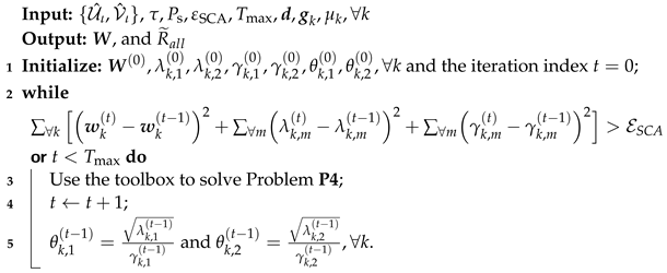
Algorithm 1: SCA ZF-based algorithm for Problem P4 under the given $\{{\widehat{\mathcal{U}}}_{\iota },{\widehat{\mathcal{V}}}_{\iota }\}$.

Algorithm 2 provides the complete process for solving Problem P1. Before executing Algorithm 1, in Step 4, we add a feasibility check. This is because, regardless of whether $n_{\mathrm{s}}{\mathit{g}}_k^T{\mathit{w}}_k$ is greater than 0, the inequality $\frac{n_{\mathrm{s}}{\mathit{g}}_k^T{\mathit{w}}_k}{\sqrt{{\lambda }_{k,1}}}\ge \frac{n_{\mathrm{s}}{\mathit{g}}_k^T{\mathit{w}}_k}{\sqrt{{\lambda }_{k,2}}},\forall k$ always exists. By preliminarily assessing feasibility, we can reduce the possibilities for discussion and decrease the likelihood of the program entering an infinite loop.    

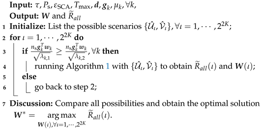
Algorithm 2: The proposed algorithm for Problem P1.

In Algorithm 1, we specify the iteration precision of SCA to ${\epsilon }_{\mathrm{SCA}}$, which requires $\mathcal{O}\left(log\left(1/{\epsilon }_{\mathrm{SCA}}\right)\right)$ iterations to be performed. In each iteration process, the MATLAB toolbox is used to resolve Problem P4, whose time complexity is $\mathcal{O}\left(\sqrt{{\mathsf{\Omega }}_{\mathrm{v}}}max{\left\{{\mathsf{\Omega }}_{\mathrm{c}},{\mathsf{\Omega }}_{\mathrm{v}}\right\}}^4\right)$ [35]. Here, ${\mathsf{\Omega }}_{\mathrm{v}}$ represents the number of variables, and ${\mathsf{\Omega }}_{\mathrm{c}}$ represents the number of constraints. For Problem P4, ${\mathsf{\Omega }}_{\mathrm{v}}=NK+4K$ and ${\mathsf{\Omega }}_{\mathrm{c}}=6K+2N$. Then, the overall computational complexity of Algorithm 1 is $\mathcal{O}\left({(NK+4K)}^{4.5}log\left(1/{\epsilon }_{\mathrm{SCA}}\right)\right)$. Algorithm 2 requires analysis of $3^K$ possibilities, meaning Algorithm 1 needs to be run $3^K$ times. Therefore, the overall computational complexity of Algorithm 2 is $\mathcal{O}\left(3^K{\left(NK\right)}^{4.5}log\left(1/{\epsilon }_{\mathrm{SCA}}\right)\right)$.

As the number of users increases, the computational complexity of Algorithm 2 rapidly escalates. Considering the properties of the function $\mathcal{F}(·)$, we can propose the following proposition.

Proposition 3. 

The ${\gamma }_{k,1}$,${\gamma }_{k,2}$ corresponding to the user with a better product of the channel state and the weight coefficient will preferentially fall within the convex interval of the function $\mathcal{F}(·)$.

Proposition 3 is easily understandable: when resources are constrained, allocating the majority of resources to users with better states can yield higher overall benefits. According to Proposition 2, under the optimal solution, ${\gamma }_{k,1}$,${\gamma }_{k,2}$ must be non-negative. Moreover, as $\mathcal{F}(·)$ monotonically decreases in the positive half-axis, resources will prioritize, placing more ${\gamma }_{k,1}$,${\gamma }_{k,2}$ values within the convex intervals. Therefore, we can use the CSI and weight distribution to pre-sort K users. Then, we can discuss the possibilities of the number of users in concave intervals, ranging from 0 to K users, corresponding to $K+1$ potential distributions of ${\gamma }_{k,1}$,${\gamma }_{k,2}$. We summarize the simplified algorithmic process in Algorithm 3, reducing the overall algorithm complexity to $\mathcal{O}\left(2K{\left(NK\right)}^{4.5}log\left(1/{\epsilon }_{\mathrm{SCA}}\right)\right)$.    

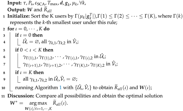
Algorithm 3: The proposed low-complexity algorithm for Problem P1.

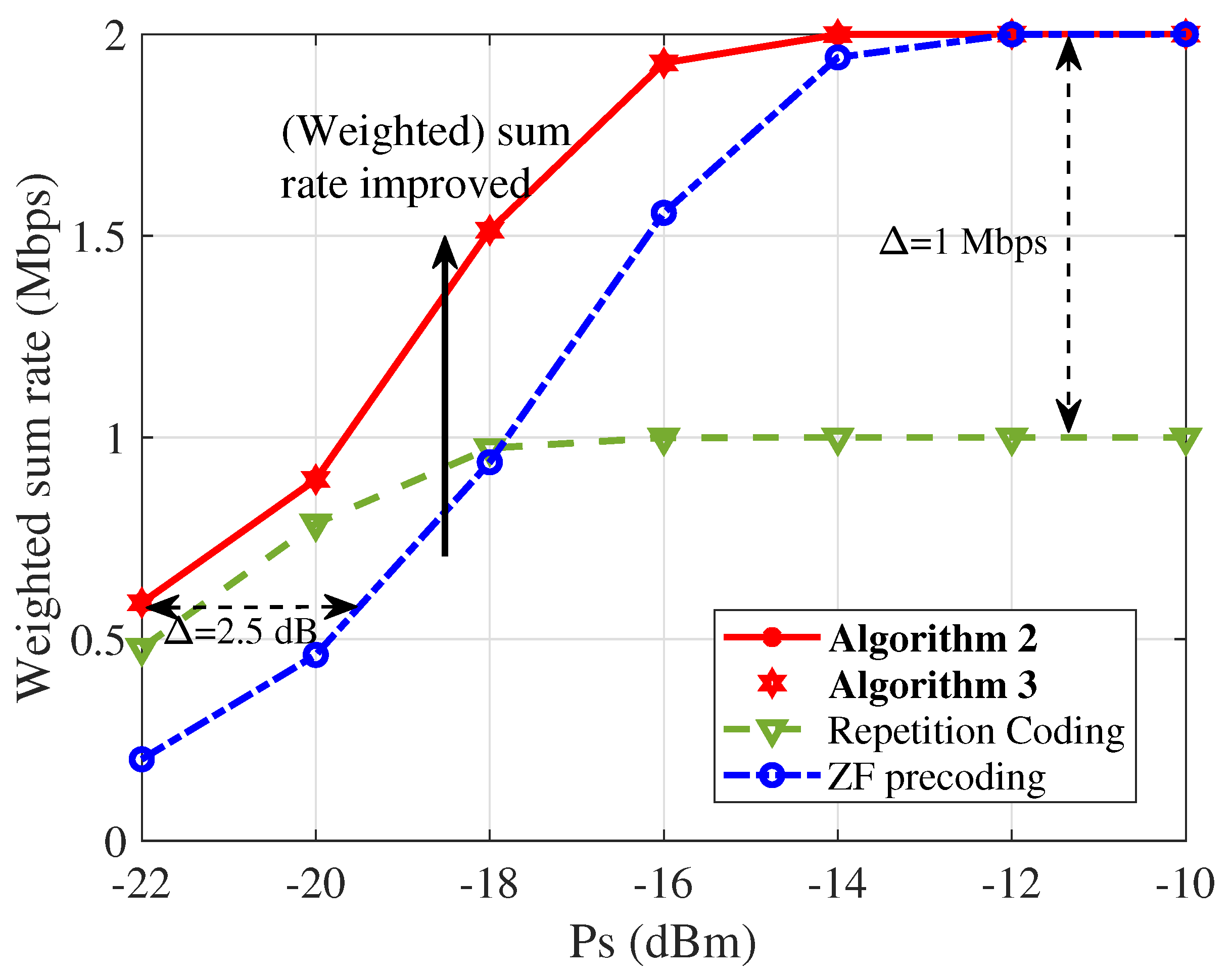
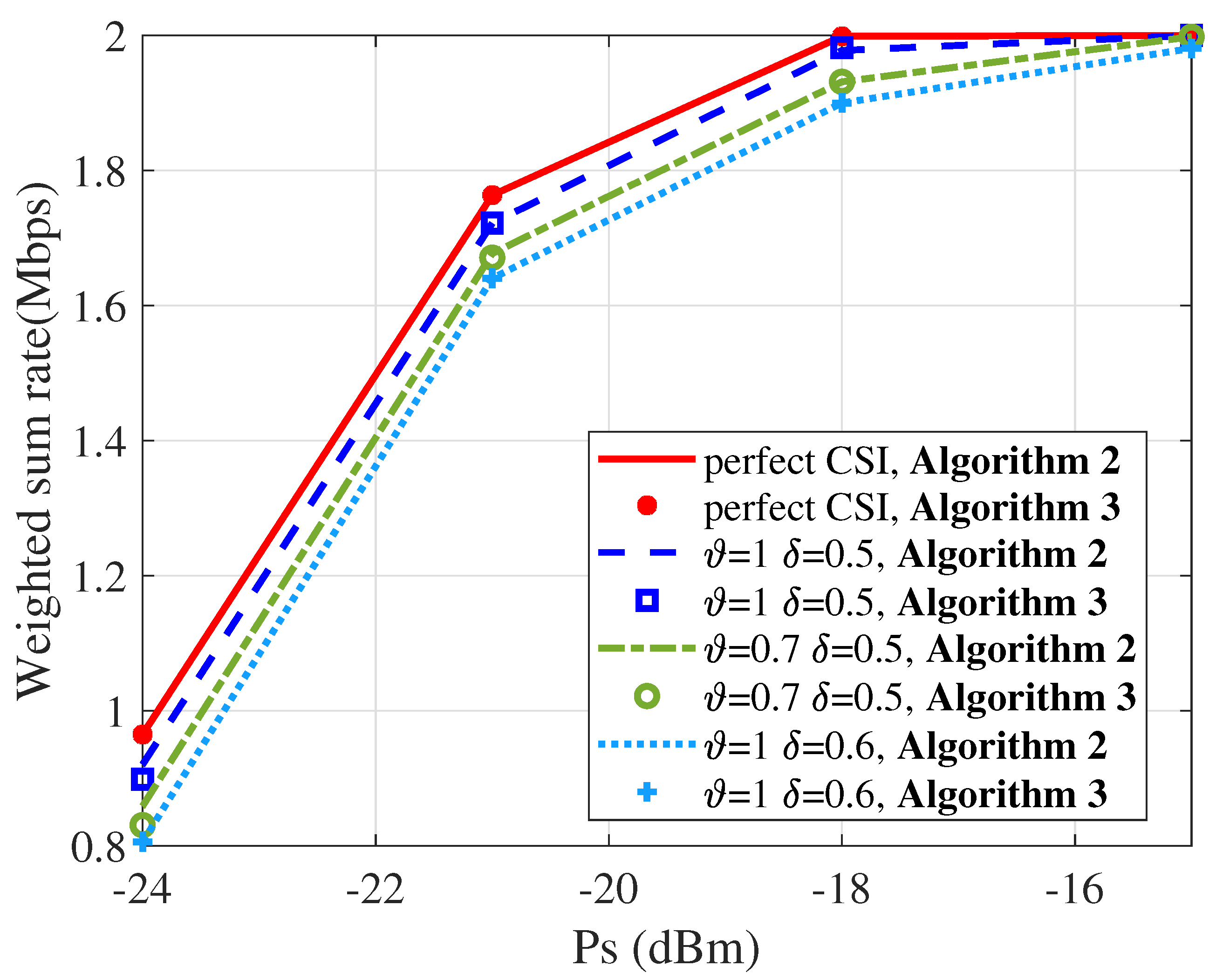
5. Numerical Results

In this section, we provide the simulation results of Algorithms 2 and 3 in the downlink MU-PhC-MIMO VLC system. The indoor space size we consider is $5\times 5\times 3$ m³. We assume the center of the ceiling to be $(2.5,2.5)$ m and evenly place N LED arrays with a grid size of $(\Delta x,\Delta y)=(0.1,0.1)$ m on the ceiling [36]. All receiving users are located on the same flat floor with a height of $0.85$ m. For the sake of generality, we assume uniformity in the weight parameters of all users during the weight-setting process, i.e., ${\mu }_k=1,\forall k$. The specific numerical values for the other parameters involved in the simulation process are presented in Table 1. The wavelength falls within the blue light range of the visible spectrum and is supported by current manufacturing processes for LEDs. The symbol duration is set to 1 $\mathsf{\mu }$s to disregard the impact of dead time effects [32]. The remaining parameter settings are adopted from [24,37].

Table 1. Simulation parameters of the system [24,37].

Parameter	Value
Visible light wavelength (v)	450 nm
Symbol duration ($\tau$)	1 $\mathsf{\mu }$s
The receiving area of the PD ($A_r$)	1 cm2
PD field of view (${\psi }_{\mathrm{F}\mathrm{o}\mathrm{V}}$)	60°
LED semi-angle (${\phi }_{1/2}$)	60°
Optical filter gain $\left(T\left({\psi }_{i,k}\right)\right)$	1
Refractive index (o)	1.5
Quantum efficiency ($\zeta$)	0.54
Background radiation power per slot ($P_{\mathrm{b}}$)	−75 dBm [38]

To the best of our knowledge, there is currently no literature exploring the achievable rates of MIMO systems affected by signal-dependent Poison shot noises, as presented in this paper. Hence, we borrow the classic ZF precoding design and repetition coding scheme from AWGN systems as benchmarks for our algorithms:

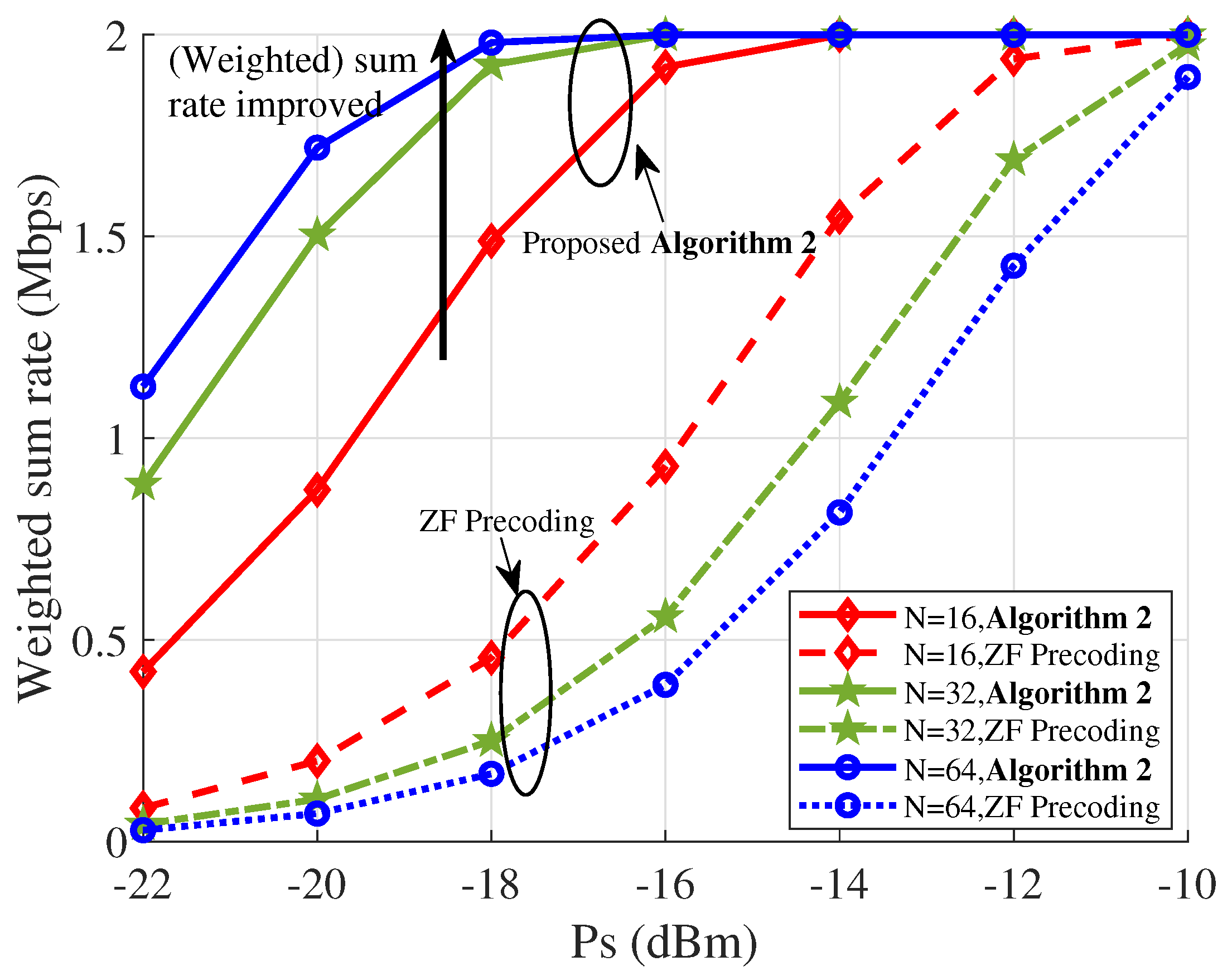
• ZF precoding [5]: We adopt the commonly used ZF precoding scheme under AWGN systems. The specific calculation method is as follows: ${\mathit{W}}_{\mathrm{ZF}}={\mathit{G}}^T{\left(\mathit{G}{\mathit{G}}^T\right)}^{-1}$ and $\mathit{G}={\left[{\mathit{g}}_1,\cdots ,{\mathit{g}}_K\right]}^T$. We rigorously check that ${\mathit{W}}_{\mathrm{ZF}}$ complies with the constraints C1–C4 in (16). If it does not meet the requirements, we normalize ${\mathit{W}}_{\mathrm{ZF}}$, i.e., ${\mathit{W}}_{\mathrm{ZF}}=\frac{{\mathit{W}}_{\mathrm{ZF}}}{\left|\right|{\mathit{W}}_{\mathrm{ZF}}{\left|\right|}_{\infty }}$. By substituting ${\mathit{W}}_{\mathrm{ZF}}$ into (15), the corresponding (weighted) sum rate can be obtained.
• Repetition coding [39]: We select the user with the best channel condition and utilize all LED arrays to transmit single-stream data to that user. This configuration establishes a MIMO framework serving a single user.

Figure 2 compares the performance of the system’s (weighted) sum rate using different algorithms as the peak power per symbol $P_{\mathrm{s}}$ increases, where $N=8$ and $K=4$. We set the upper limit of the LED’s transmission power to $P_{\max }=5\mathrm{dBm}$, the bias power to $P_{\mathrm{d}}=-5\mathrm{dBm}$, and $\mathit{d}$ can be obtained based on $\mathit{d}=\frac{P_{\mathrm{d}}\tau }{ħv}$. We can observe that the proposed Algorithms 2 and 3 are better than the ZF precoding and repetition coding schemes because the classic schemes are not suitable for MIMO systems limited by Poisson shot noises. In the case of low $P_{\mathrm{s}}$, Algorithms 2 and 3 can improve by 2.5 dB compared to the ZF precoding method. The repetition coding scheme tends to a fixed value as $P_{\mathrm{s}}$ continues to increase. This is because this scheme serves a single user and has an upper limit on the achievable rate. On the other hand, we can observe that the proposed Algorithms 2 and 3 are almost consistent, indicating that Algorithm 3 can play a certain role in simplifying Algorithm 2.

Figure 2. Sum-rate performance of the proposed MU-PhC-MIMO VLC system with $N=4$ and $K=2$ using different algorithms.

Figure 3 shows the sum-rate performance of Algorithm 2 and the ZF precoding method as $P_{\mathrm{s}}$ increases, where $K=2$ and $N=16,32,64$. We can observe that an increase in the number of active LEDs in Algorithm 2 leads to an improvement in the system’s (weighted) sum rate. In other words, to achieve the same (weighted) sum rate, increasing the number of LED arrays can save transmit peak power. This is because it leverages the properties of transmit diversity. However, in the ZF precoding scheme, as N increases, the elements become smaller when calculating the pseudo-inverse of the channel matrix, leading to a gradual deterioration in performance.

Figure 3. Sum-rate performance of the proposed MU-PhC-MIMO VLC system with $K=2$ under different numbers of LED arrays.

Figure 4 depicts the system’s (weighted) sum rate based on Algorithm 2 under various DC bias power scenarios, where $N=16,K=4,$ and $P_{\mathrm{d}}=-5,-6.2,-8,-11$ dBm. It is evident that an increase in the DC bias results in a reduction in the system’s (weighted) sum rate. This indicates that the DC bias causes interference at the receivers. Therefore, in practical applications, selecting an appropriate value for the bias becomes crucial. It should comply with the non-negativity requirement of the transmitted signal while minimizing the impact on the receivers’ rates.

Figure 4. Sum-rate performance of the proposed MU-PhC-MIMO VLC system with $N=16$ and $K=4$ under different DC bias power scenarios.

Figure 5 demonstrates the impact of increasing user numbers, resulting in multiple streams on the system’s (weighted) sum rate for the proposed Algorithms 2 and 3, where $N=16$ and $K=2,3,4,5$. It can be observed that Algorithm 3 performs slightly lower than Algorithm 2 at low power levels. However, with the growth of the transmit peak power, the gap between them gradually diminishes, approaching convergence. At lower transmit peak power, ${\gamma }_{k,1}$,${\gamma }_{k,2},\forall k$ cannot simultaneously fall within the convex intervals due to the limited considerations in Algorithm 3, resulting in gaps. Yet, with sufficient transmit peak power, the likelihood of being within the convex intervals increases. Algorithm 3 accounts for this possibility, thus converging with the performance of Algorithm 2. Additionally, we also notice that the performance diminishes at lower transmit-power levels as the number of users increases. However, increasing power demonstrates the advantages of multi-user scenarios. This is also a consequence of power limitations.

Figure 5. Sum-rate performance of the proposed MU-PhC-MIMO VLC system with $N=16$ for different numbers of users.

Figure 6 plots the convergence behavior of Algorithm 1. Figure 6a depicts the iterative convergence of Algorithm 1 with five distinct $\{{\widehat{\mathcal{U}}}_{\iota },{\widehat{\mathcal{V}}}_{\iota }\}$ scenarios selected in Algorithm 3 when $P_{\mathrm{s}}=-16$ dBm. It can be observed that under the various $\{{\widehat{\mathcal{U}}}_{\iota },{\widehat{\mathcal{V}}}_{\iota }\}$ scenarios, the system’s (weighted) sum rate shows a step-like growth pattern. Figure 6b displays the iterative process of running Algorithm 1 corresponding to the optimal solutions obtained by Algorithm 3 under various transmit peak power levels, where $P_{\mathrm{s}}=-24,-20,-18,-16$ dBm. The comparison reveals that at lower power conditions, fewer occurrences of ${\gamma }_{k,1}$,${\gamma }_{k,2},\forall k$ fall within the convex intervals. However, as the power increases, the occurrences of ${\gamma }_{k,1}$,${\gamma }_{k,2},\forall k$ within these intervals gradually rise, confirming our hypothesis in Proposition 3. Figure 6a,b collectively demonstrate that after a few iterations, Algorithm 1 converges to a solution, substantiating the effectiveness of the algorithm to a certain extent.

Figure 6. Convergence of Algorithm 1. (a) Running Algorithm 1 with five different $\{{\widehat{\mathcal{U}}}_{\iota },{\widehat{\mathcal{V}}}_{\iota }\}$ scenarios determined by Algorithm 3 under $P_{\mathrm{s}}=-16$ dBm. (b) Running Algorithm 3 for different transmit-power scenarios and illustrating the convergence process of Algorithm 1 corresponding to the optimal solution cases.

Figure 7 shows the numerical results under scenarios where the transmitter possesses imperfect CSI because of the CSI estimation errors or delayed feedback from the receiver. We assume that these errors follow an independent Gaussian distribution, represented as ${\epsilon }_{\mathrm{CSI}}\sim \mathcal{N}(0,{\sigma }_{\epsilon }^2)$. The variances of these errors are represented by the error parameters $\delta$ and $\vartheta$, i.e., ${\sigma }_{\epsilon }={\left(\delta g\right)}^{\vartheta }$ [32]. We present the simulation results for four different error levels, where $N=4,K=2$, and $P_d=-13$ dBm. The legend ’perfect CSI’ represents the case where the variance is 0. It is observed that both Algorithms 2 and 3 exhibit good robustness. Furthermore, the imperfections in the channel can be mitigated by increasing the transmit power.

Figure 7. Sum-rate performance of the proposed MU-PhC-MIMO VLC system under imperfect CSI.

6. Conclusions

We have utilized the zero-forcing concept to maximize the weighted sum rate of an interference-free downlink MU-PhC-MIMO VLC system. First, we derive the precise expression for the system’s weighted sum rate and propose the rate expression based on the ZF scheme. Furthermore, we employ mathematical tools to accomplish Gaussian approximations. Then, by employing variable substitutions and SCA, we recursively convexify and maximize the new objective. By comparing various possibilities, we arrive at the optimal solution for the complete optimization problem. After extensive simulation validation, our algorithms exhibit performance that allows saving 2.5 dB of transmit peak power compared to the classical ZF precoding scheme in low-transmit-power scenarios. Moreover, at higher power levels, the system’s weighted sum rate significantly outperforms the repetition coding scheme. Additionally, the two proposed algorithms exhibit almost identical performance and showcase improved weighted sum rates with more active LED arrays and lower DC bias power.

References

1. Wang, C.X.; Haider, F.; Gao, X.; You, X.H.; Yang, Y.; Yuan, D.; Hepsaydir, E. Cellular architecture and key technologies for 5G wireless communication networks. IEEE Commun. Mag. 2014, 52, 122–130. [Google Scholar] [CrossRef]
2. Xu, Z.; Liu, W.; Wang, Z.; Hanzo, L. Petahertz communication: Harmonizing optical spectra for wireless communications. Digit. Commun. Netw. 2021, 7, 605–614. [Google Scholar] [CrossRef]
3. Yang, Z.; Chen, M.; Saad, W.; Hong, C.S.; Shikh-Bahaei, M. Energy efficient federated learning over wireless communication networks. IEEE Trans. Wirel. Commun. 2020, 20, 1935–1949. [Google Scholar] [CrossRef]
4. Feng, R.; Kong, J.; Guo, X.; Jiang, W.; Xie, S. Joint precoding and power allocation in FSO channel with signal-dependent noise. Appl. Opt. 2023, 62, 6060–6071. [Google Scholar] [CrossRef]
5. Ge, H.; Zhou, X.; Chen, Y.; Zhang, J.; Ni, W.; Wang, X.; Zheng, L. Shot-noise-limited photon-counting precoding scheme for MIMO ultraviolet communication in atmospheric turbulence. Opt. Express 2023, 31, 426–441. [Google Scholar] [CrossRef]
6. Ahmadypour, N.; Gohari, A. Transmission of a bit over a discrete Poisson channel with memory. Digit. Commun. Netw. 2021, 67, 4710–4727. [Google Scholar]
7. Zhang, J.Z.; Ke, K.; Ren, J. Multiuser robust transceiver design for indoor VLC with noisy channel state information. In Proceedings of the IEEE International Conference on Progress in Informatics and Computing (PIC), Shanghai, China, 18–20 December 2020; pp. 289–293. [Google Scholar]
8. Ma, X.; Jin, X.; Deng, J.; Jin, M.; Gong, C.; Xu, Z. Symbol-level precoding for multiuser visible light communication. In Proceedings of the 11th International Conference on Wireless Communications and Signal Processing (WCSP), Xi’an, China, 23–25 October 2019; pp. 1–6. [Google Scholar]
9. Guo, Y.; Xiong, K.; Lu, Y.; Gao, B.; Fan, P.; Letaief, K.B. SLIPT-enabled multi-LED MU-MISO VLC networks: Joint beamforming and DC bias optimization. IEEE Trans. Green Commun. Netw. 2023, 7, 1104–1120. [Google Scholar] [CrossRef]
10. Shen, H.; Deng, Y.; Xu, W.; Zhao, C. Rate-maximized zero-forcing beamforming for VLC multiuser MISO downlinks. IEEE Photonics J. 2016, 8, 7901913. [Google Scholar] [CrossRef]
11. Shen, H.; Xu, W.; Zhao, K.; Bai, F.; Zhao, C. Non-alternating globally optimal MMSE precoding for multiuser VLC downlinks. IEEE Commun. Lett. 2019, 23, 608–611. [Google Scholar] [CrossRef]
12. Morales-Céspedes, M.; Haas, H.; Armada, A.G. Optimization of the receiving orientation angle for zero-forcing precoding in VLC. IEEE Commun. Lett. 2020, 25, 921–925. [Google Scholar] [CrossRef]
13. Zhao, L.; Cai, K.; Jiang, M. Multiuser precoded MIMO visible light communication systems enabling spatial dimming. J. Light. Technol. 2020, 38, 5624–5634. [Google Scholar] [CrossRef]
14. Ma, H.; Mostafa, A.; Lampe, L.; Hranilovic, S. Coordinated beamforming for downlink visible light communication networks. IEEE Trans. Commun. 2018, 66, 3571–3582. [Google Scholar] [CrossRef]
15. Sifaou, H.; Kammoun, A.; Park, K.H.; Alouini, M.S. Robust transceivers design for multi-stream multi-user MIMO visible light communication. IEEE Access 2017, 5, 26387–26399. [Google Scholar] [CrossRef]
16. Zhao, S.; Li, Q.; Tian, M. Capacity-maximized transmitter precoding for MU MIMO VLC systems with bounded channel uncertainties. IEEE Syst. J. 2020, 14, 5144–5147. [Google Scholar] [CrossRef]
17. Wang, Z.Y.; Yu, H.Y.; Wang, D.M. Energy-efficient precoding design for multiuser MISO VLC systems based on joint detection. IEEE Access 2019, 7, 16274–16280. [Google Scholar] [CrossRef]
18. Yu, Z.; Baxley, R.J.; Zhou, G.T. Multi-user MISO broadcasting for indoor visible light communication. In Proceedings of the IEEE International Conference on Acoustics, Speech and Signal Processing, Vancouver, BC, Canada, 26–31 May 2013; pp. 4849–4853. [Google Scholar]
19. Kim, J.H.; Olson, A.; Govindasamy, S.; Rahaim, M.B. An approach for Tomlinson-Harashima precoding in visible-light-communications systems. In Proceedings of the International Conference on Computer, Information and Telecommunication Systems (CITS), Colmar, France, 11–13 July 2018; pp. 1–5. [Google Scholar]
20. Wang, C.; Yang, Y.; Yang, Z.; Feng, C.; Cheng, J.; Guo, C. Joint SIC-based precoding and sub-connected architecture design for MIMO VLC systems. IEEE Trans. Commun. 2022, 71, 1044–1058. [Google Scholar] [CrossRef]
21. Feng, Z.; Guo, C.; Ghassemlooy, Z.; Yang, Y. The spatial dimming scheme for the MU-MIMO-OFDM VLC system. IEEE Photonics J. 2018, 10, 7907013. [Google Scholar] [CrossRef]
22. Wang, Q.; Wang, Z.; Dai, L. Multiuser MIMO-OFDM for visible light communications. IEEE Photonics J. 2015, 7, 7904911. [Google Scholar] [CrossRef]
23. Arya, S.; Chung, Y.H. State-of-the-art ultraviolet multiuser indoor communication over power-constrained discrete-time Poisson channels. Opt. Eng. 2020, 59, 106106. [Google Scholar] [CrossRef]
24. Arfaoui, M.A.; Ghrayeb, A.; Assi, C.M. Secrecy performance of multi-user MISO VLC broadcast channels with confidential messages. IEEE Trans. Wirel. Commun. 2018, 17, 7789–7800. [Google Scholar] [CrossRef]
25. Komine, T.; Nakagawa, M. Fundamental analysis for visible-light communication system using LED lights. IEEE Trans. Consum. Electron. 2004, 50, 100–107. [Google Scholar] [CrossRef]
26. Yang, Y.; Wang, C.; Feng, C.; Guo, C.; Cheng, J.; Zeng, Z. A generalized dimming control scheme for visible light communications. IEEE Trans. Commun. 2021, 69, 1845–1857. [Google Scholar] [CrossRef]
27. Keskin, M.F.; Sezer, A.D.; Gezici, S. Localization via visible light systems. Proc. IEEE Inst. Electr. Electron. Eng. 2018, 106, 1063–1088. [Google Scholar] [CrossRef]
28. Gong, C.; Xu, Z. Channel estimation and signal detection for optical wireless scattering communication with inter-symbol interference. IEEE Trans. Wirel. Commun. 2015, 14, 5326–5337. [Google Scholar] [CrossRef]
29. Chen, X.; Jiang, M. Adaptive statistical Bayesian MMSE channel estimation for visible light communication. IEEE Trans. Signal Process. 2016, 65, 1287–1299. [Google Scholar] [CrossRef]
30. Yesilkaya, A.; Karatalay, O.; Ogrenci, A.S.; Panayirci, E. Channel estimation for visible light communications using neural networks. In Proceedings of the International Joint Conference on Neural Networks (IJCNN), Vancouver, BC, Canada, 24–29 July 2016; pp. 320–325. [Google Scholar]
31. Fray, S.; Johnson, F.A.; Jones, R.; McLean, T.P.; Pike, E.R. Photon-counting distributions of modulated laser beams. Phys. Rev. 1967, 153, 357–359. [Google Scholar] [CrossRef]
32. Chen, Y.; Zhou, X.; Ni, W.; Hossain, E.; Wang, X. Optimal power allocation for multiuser photon-counting underwater optical wireless communications under poisson shot noise. IEEE Trans. Commun. 2023, 71, 2230–2245. [Google Scholar] [CrossRef]
33. Grant, M.; Boyd, S. CVX: MATLAB Software for Disciplined Convex Programming, Version 2.2. Available online: http://cvxr.com/cvx (accessed on 1 January 2020).
34. Marks, B.R.; Wright, G.P. A general inner approximation algorithm for nonconvex mathematical programs. Oper. Res. 1978, 26, 681–683. [Google Scholar] [CrossRef]
35. Sun, C.; Ni, W.; Bu, Z.; Wang, X. Energy minimization for intelligent reflecting surface-assisted mobile edge computing. IEEE Trans. Wirel. Commun. 2022, 21, 6329–6344. [Google Scholar] [CrossRef]
36. Arfaoui, M.A.; Zaid, H.; Rezki, Z.; Ghrayeb, A.; Chaaban, A.; Alouini, M.S. Artificial noise-based beamforming for the MISO VLC wiretap channel. IEEE Trans. Commun. 2018, 67, 2866–2879. [Google Scholar] [CrossRef]
37. Mostafa, A.; Lampe, L. Optimal and robust beamforming for secure transmission in MISO visible-light communication links. IEEE Trans. Signal Process. 2016, 64, 6501–6516. [Google Scholar] [CrossRef]
38. Han, D.; Lee, K. Ambient light noise filtering technique for multimedia high speed transmission system in MIMO-VLC. Multimed. Tools. Appl. 2021, 80, 34751–34765. [Google Scholar] [CrossRef]
39. Alhadiid, G.G.; Astuti, R.P.; Hidayat, B.; Darlis, D. Indoor visible light communication system with diversity combining and repetition code. In Proceedings of the IEEE International Conference on Signals and Systems (ICSigSys), Bandung, Indonesia, 16–18 July 2019; pp. 138–142. [Google Scholar]
40. Leemis, L.M.; McQueston, J.T. Univariate distribution relationships. Am. Stat. 2008, 62, 45–53. [Google Scholar] [CrossRef]
41. Biswas, S.; Ghassemlooy, Z.; Le-Minh, H.; Chattopadhyay, S.; Tang, X.; Lin, B. On application of a positioning system using photosensors with user mobility support in HealthCare system. Proc. Natl. Acad. Sci. India Sect. A Phys. Sci. 2023, 93, 121–133. [Google Scholar] [CrossRef]