Componentwise Perturbation Analysis of the Singular Value Decomposition of a Matrix

Abstract

A rigorous perturbation analysis is presented for the singular value decomposition (SVD) of a real matrix with full column rank. It is proved that the SVD perturbation problem is well posed only when the singular values are distinct. The analysis involves the solution of symmetric coupled systems of linear equations. It produces asymptotic (local) componentwise perturbation bounds on the entries of the orthogonal matrices participating in the decomposition of the given matrix and on its singular values. Local bounds are derived for the sensitivity of the singular subspaces measured by the angles between the unperturbed and perturbed subspaces. Determining the asymptotic bounds of the orthogonal matrices and the sensitivity of singular subspaces requires knowing only the norm of the perturbation of the given matrix. An iterative scheme is described to find global bounds on the respective perturbations, and results from numerical experiments are presented.

1. Introduction

As it is known ([1], Ch. 2), ([2], Ch. 1), ([3], Ch, 2), each $m\times n,m\ge n$ matrix $A\in {\mathbb{R}}^{m\times n}$ can be represented by the singular value decomposition (SVD) in the factorized form

$$A=U\Sigma V^T,$$

(1)

where the $m\times m$ matrix U and the $n\times n$ matrix V are orthogonal and the $m\times n$ matrix $\Sigma$ is diagonal:

$$\Sigma =\left[\begin{array}{c}{\Sigma }_n\\ 0_{(m-n)\times n)}\end{array}\right],{\Sigma }_n=\mathrm{diag}\left({\sigma }_1,{\sigma }_2,\dots ,{\sigma }_n\right).$$

The numbers ${\sigma }_i\ge 0$ are called singular values of the matrix A. The columns of

$$U:=[u_1,u_2,\dots ,u_m],u_j\in {\mathbb{R}}^m,$$

are called left singular vectors and the columns of

$$V:=[v_1,v_2,\dots ,v_n],v_j\in {\mathbb{R}}^n$$

are the right singular vectors. The subspaces spanned by sets of left and right singular vectors are called left and right singular subspaces, respectively.

The singular value decomposition has a long and interesting history described in [4].

The SVD has many properties, making it an invaluable tool in matrix analysis and matrix computations; see the references cited above. Among them is that the rank r of A equals the number of its nonzero singular values and the equality ${\parallel A\parallel }_2={\sigma }_{\max }$. The usual assumption is that by an appropriate ordering of the columns $u_j$ and $v_j$, the singular values appear in the order

$${\sigma }_{\max }:={\sigma }_1\ge {\sigma }_2\ge \dots \ge {\sigma }_n:={\sigma }_{min}.$$

If some of the singular values are equal to zero, then A has $r<n$ linearly independent columns, and the matrix $\Sigma$ in (1) can be represented as

$$\Sigma =\left[\begin{array}{cc}{\Sigma }_r& 0_{r\times (n-r)}\\ 0_{(m-r)\times r}& 0_{(m-r)\times (n-r)}\end{array}\right],{\Sigma }_r=\mathrm{diag}\left({\sigma }_1,{\sigma }_2,\dots ,{\sigma }_r\right).$$

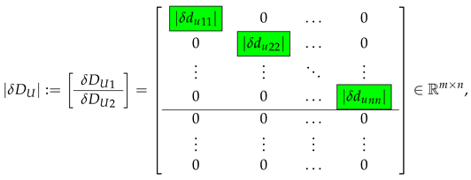
Further, we shall consider the case $r=n$, i.e., assume that the matrix A is of full column rank.

This paper concerns the case when the matrix A is subject to an additive perturbation $\delta A$. In such a case, there exists another pair of orthogonal matrices $\tilde{U}$ and $\tilde{V}$ and a diagonal matrix $\tilde{\Sigma }$, such that

$$\tilde{A}:=A+\delta A=\tilde{U}\tilde{\Sigma }{\tilde{V}}^T.$$

(2)

The perturbation analysis of the singular value decomposition consists in determining the changes in the quantities related to the elements of the decomposition due to the perturbation $\delta A$. This includes determining bounds on the changes of the entries of the orthogonal matrices that reduce the original matrix to diagonal form and bounds on the perturbations of the singular values. Hence, the analysis aims to find bounds on the sizes of $\delta U=\tilde{U}-U$, $\delta V=\tilde{V}-V$, and $\delta \Sigma =\tilde{\Sigma }-\Sigma$ as functions of the size of $\delta A$. It should be emphasized that problems of such a kind arise in most singular value decomposition applications. The most important application of the perturbation analysis is to assess the accuracy of the computed SVD since each algorithm for its determination produces the SVD of $A+\delta A$, not of A, where the size of $\delta A$ depends on the properties of the floating point arithmetic used and the corresponding algorithm. Knowing the size of $\delta A$, we may use the perturbation bounds to estimate the difference between the actual and computed elements of the decomposition. For a deep and systematic presentation of the matrix perturbation theory and its use in accuracy estimation, the reader is referred to the books of Stewart [2], Stewart and Sun [5], and Wilkinson [6].

According to Weyl’s theorem ([2], Ch. 1), we have that

$$|\delta {\sigma }_i|=|{\tilde{\sigma }}_i-{\sigma }_i|\le {\parallel \delta A\parallel }_2,i=1,2,\dots ,n,$$

(3)

which shows that the singular values are perturbed by no more than the 2-norm of the perturbation of A; i.e., the singular values are always well conditioned. The SVD perturbation analysis is well defined if the matrix A is of full column rank n; i.e., ${\sigma }_{min}\ne 0$, since otherwise, the corresponding left singular vector is undetermined.

The size of the perturbations $\delta A$, $\delta U$, $\delta V$, and $\delta \Sigma$ is usually measured by using some of the matrix norms, which leads to the so-called normwise perturbation analysis. In several cases, we are interested in the size of the perturbations of the individual entries of $\delta U$, $\delta V$, and $\delta \Sigma$, so that it is necessary to implement a componentwise perturbation analysis [7]. This analysis has an advantage when the individual components of $\delta U$, $\delta V$, and $\delta \Sigma$ differ significantly in magnitude, and the normwise estimates do not produce tight bounds on the perturbations.

The literature on the perturbation theory of the singular value decomposition is significant. The first results on this topic are obtained by Wedin [8] and Stewart [9], who developed estimates of the sensitivity of pairs of singular subspaces (see also ([5], Ch. V)). Other results concerning the sensitivity of the singular vectors and singular subspaces are obtained in [10,11], and a survey on the perturbation theory of the SVD until 1990 can be found in [12]. Using the technique of perturbation expansions for invariant subspaces, Sun [13] derived perturbation bounds for a pair of singular subspaces that improved the bounds obtained in [9] and contained as a special case the bounds presented in [11]. A perturbation theory for the singular values and singular subspaces of diagonally dominant matrices, including graded matrices, is presented in [14], and optimal perturbation bounds for the case of structured perturbations are derived in [15]. The seminal paper by Demmel and his co-authors [16] contains a perturbation theory that provides relative perturbation bounds for the singular values and singular subspaces for different classes of matrices. The problem of backward error analysis of SVD algorithms is discussed in [17]. High-accuracy algorithms for computing SVD are proposed by Drmač and Veselić in [18,19] and implemented in the LAPACK package [20]. An improvement in the results of [8] is presented in [21]. Several results concerning the sensitivity of the SVD are summarized in the survey [22], and a reach bibliography on the accurate computation of SVD can be found in [23]. Finally, some recent applications of SVD are described in [24,25]. It should be pointed out that the available SVD perturbation theory provides bounds on the sensitivity of the singular vectors and singular subspaces but does not provide perturbation bounds on the individual entries of the matrices U and V. Such bounds are important in several applications, and this fact justifies the opinion that apart from the large number of results about the sensitivity of the singular values and singular vectors, a complete componentwise perturbation analysis of the SVD is not available up to the moment.

This paper presents a rigorous perturbation analysis of the orthogonal matrices, singular subspaces, and singular values of a real matrix of full column rank. It is proved that the SVD perturbation problem is well posed only in the case of distinct (simple) singular values. The analysis produces asymptotic (local) componentwise perturbation bounds of the entries of the orthogonal matrices U and V and the singular values of the given matrix. Local bounds are derived for the sensitivity of a pair of singular subspaces measured by the angles between the unperturbed and perturbed subspaces. An iterative scheme is described to find global bounds on the respective perturbations, and the results of numerical experiments are presented. The analysis performed in the paper implements the same methodology as the one used previously in [26] to determine componentwise perturbation bounds of the QR decomposition of a matrix. However, the SVD perturbation analysis has some distinctive features, making it a self-dependent problem.

The paper is organized as follows. In Section 2, we derive the basic nonlinear algebraic equations used to perform the perturbation analysis of the SVD. After introducing in Section 3 the perturbation parameters that determine the perturbations of the matrices U and V, we derive a symmetric system of coupled equations for these parameters in Section 4. The solution to the equations for the first-order terms of the perturbation parameters allows us to find asymptotic bounds on the parameters in Section 5, on the singular values in Section 6, and on the perturbations of the matrices U and V in Section 7. Using the bounds on the perturbation parameters in Section 8, we derive bounds on the sensitivity of the singular subspaces. In Section 9, we develop an iterative scheme for finding global bounds on the perturbations, and in Section 10 we present the results of some numerical experiments illustrating the proposed analysis. Some conclusions are drawn in Section 11.

2. Basic Equations

The perturbed singular value decomposition of A (2) can be written as

$${\tilde{U}}^T\tilde{A}\tilde{V}=\tilde{\Sigma },$$

(4)

where

$$\begin{array}{ccc}\hfill \tilde{U}& =& U+\delta U:=[{\tilde{u}}_1,{\tilde{u}}_2,\dots ,{\tilde{u}}_m],{\tilde{u}}_j\in {\mathbb{R}}^m,\hfill \\ \hfill \delta U& :=& [\delta u_1,\delta u_2,\dots ,\delta u_m],\delta u_j\in {\mathbb{R}}^m,\hfill \\ \hfill {\tilde{u}}_j& =& u_j+\delta u_j,j=1,2,\dots ,m,\hfill \\ \hfill \tilde{V}& =& V+\delta V:=[{\tilde{v}}_1,{\tilde{v}}_2,\dots ,{\tilde{v}}_n],{\tilde{v}}_j\in {\mathbb{R}}^n,\hfill \\ \hfill \delta V& :=& [\delta v_1,\delta v_2,\dots ,\delta v_n],\delta v_j\in {\mathbb{R}}^n,\hfill \\ \hfill {\tilde{v}}_j& =& v_j+\delta v_j,j=1,2,\dots ,n,\hfill \end{array}$$

and

$$\begin{array}{ccc}\hfill \tilde{\Sigma }& =& \Sigma +\delta \Sigma =\left[\begin{array}{c}{\tilde{\Sigma }}_n\\ 0\end{array}\right],\hfill \\ \hfill {\tilde{\Sigma }}_n& =& {\Sigma }_n+\delta {\Sigma }_n=\mathrm{diag}({\tilde{\sigma }}_1,{\tilde{\sigma }}_2,\dots ,{\tilde{\sigma }}_n),\hfill \\ \hfill \delta {\Sigma }_n& =& \mathrm{diag}(\delta {\sigma }_1,\delta {\sigma }_2,\dots ,\delta {\sigma }_n),\hfill \\ \hfill {\tilde{\sigma }}_i& =& {\sigma }_i+\delta {\sigma }_i.\hfill \end{array}$$

Equation (4) is rewritten as

$$\delta U^{T}AV+U^{T}A\delta V+\delta F=\left[\begin{array}{c}\delta {\Sigma }_n\\ 0_{(m-n)\times n}\end{array}\right]+{\Delta }_0,$$

(5)

where $\delta F=U^T\delta AV$ and the matrix ${\Delta }_0$

$${\Delta }_0=-\delta U^{T}A\delta V-U^T\delta A\delta V-\delta U^T\delta AV-\delta U^T\delta A\delta V\in {\mathbb{R}}^{m\times n}$$

contains only higher-order terms in the elements of $\delta A$, $\delta U$, and $\delta V$.

Let the matrices U and $\delta U$ be separated as $U=[U_1,U_2],U_1\in {\mathbb{R}}^{m\times n}$ and $\delta U=[\delta U_1,\delta U_2],$$\delta U_1\in {\mathbb{R}}^{m\times n}$, respectively. Since the matrix A can be represented as $A=U_1{\Sigma }_n{V}^T$, the matrix $U_2$ is not well determined but should satisfy the orthogonality condition ${[U_1,U_2]}^T[U_1,U_2]=I_m$. The perturbation $\delta U_2$ is also undefined so that we can bound only the perturbations of the entries in the first n columns of U, i.e., the entries of $\delta U_1$. Further on, we shall use (5) to determine componentwise bounds on $\delta U_1$, $\delta V$ and $\delta {\Sigma }_n$.

3. Perturbed Orthogonal Matrices and Perturbation Parameters

In the perturbation analysis of the SVD, it is convenient to find first componentwise bounds on the entries of the matrices $\delta W_U:=U^T\delta U_1$ and $\delta W_V:=V^T\delta V$, which are related to the corresponding perturbations $\delta U_1$ and $\delta V$ by orthogonal transformations. The implementation of the matrices $\delta W_U$ and $\delta W_V$ allows us to find bounds on

$$\delta U_1=U\delta W_U$$

(6)

and

$$\delta V=V\delta W_V$$

(7)

using orthogonal transformations without increasing the norms of $\delta W_U$ and $\delta W_V$. This helps to determine bounds on $\delta U_1$ and $\delta V$, which are as tight as possible.

First, consider the matrix

$$\delta W_U=U^T\delta U_1=\left[\begin{array}{cccc}{u}_1^T\delta u_1& u_1^T\delta u_2& \dots & u_1^T\delta u_n\\ u_2^T\delta u_1& u_2^T\delta u_2& \dots & u_2^T\delta u_n\\ ⋮& ⋮& ⋮& ⋮\\ u_n^T\delta u_1& u_n^T\delta u_2& \dots & u_n^T\delta u_n\\ u_{n+1}^T\delta u_1& u_{n+1}^T\delta u_2& \dots & u_{n+1}^T\delta u_n\\ ⋮& ⋮& ⋮& ⋮\\ u_m^T\delta u_1& u_m^T\delta u_2& \dots & u_m^T\delta u_n\end{array}\right]\in {\mathbb{R}}^{m\times n}.$$

Further on, we shall use the vector of the subdiagonal entries of the matrix $\delta W_U$,

$$\begin{array}{ccc}\hfill x& :=& {[x_1,x_2,\dots ,x_p]}^T\in {\mathbb{R}}^p,\hfill \\ & =& {[\underset{m-1}{\underbrace{u_2^T\delta u_1,u_3^T\delta u_1,\dots ,u_m^T\delta u_1}},\underset{m-2}{\underbrace{u_3^T\delta u_2,\dots ,u_m^T\delta u_2}},\dots ,\underset{m-n}{\underbrace{u_{n+1}^T\delta u_n,\dots ,u_m^T\delta u_n}}]}^T,\hfill \end{array}$$

where

$$p=\sum _{i=1}^n(m-i)=n(n-1)/2+(m-n)n=n(2m-n-1)/2.$$

As it will become clear later on, together with the orthogonality condition

$${[U_1+\delta U_1]}^T[U_1+\delta U_1]=I_n,$$

the vector x contains the whole information necessary to find the perturbation $\delta U_1$. This vector may be expressed as

$$x=\mathrm{vec}(\mathrm{Low}(\delta W_U)),$$

or, equivalently,

$$x={\Omega }_x\mathrm{vec}(\delta W_U),$$

where

$$\begin{array}{ccc}\hfill {\Omega }_x& :=& \left[\mathrm{diag}({\omega }_1,{\omega }_2,\dots ,{\omega }_n)\right]\in {\mathbb{R}}^{p\times mn},\hfill \\ \hfill {\omega }_i& :=& \left[0_{(m-i)\times i},I_{m-i}\right]\in {\mathbb{R}}^{(m-i)\times m},i=1,2,\dots ,n,\hfill \\ & & {\Omega }_x{\Omega }_x^T=I_p,{\parallel {\Omega }_x\parallel }_2=1\hfill \end{array}$$

is a matrix that “pulls out” the p elements of x from the $m·n$ elements of $\delta W_U$ (we consider $0_{0\times i}$ as an empty matrix). If, for instance, $m=6$ and $n=4$, then

$$\mathrm{Low}(\delta W_U)=\left[\begin{array}{cccc}& & & \\ \delta {w_u}_{21}& & & \\ \delta {w_u}_{31}& \delta {w_u}_{32}& & \\ \delta {w_u}_{41}& \delta {w_u}_{42}& \delta {w_u}_{43}& \\ \delta {w_u}_{51}& \delta {w_u}_{52}& \delta {w_u}_{53}& \delta {w_u}_{54}\\ \delta {w_u}_{61}& \delta {w_u}_{62}& \delta {w_u}_{63}& \delta {w_u}_{64}\end{array}\right],$$

$$\begin{array}{ccc}\hfill \mathrm{vec}(\delta W_U)& =& \left[\delta {w_u}_{11}\delta {w_u}_{21}\delta {w_u}_{31}\delta {w_u}_{41}\delta {w_u}_{51}\delta {w_u}_{61}|\right.\dots \hfill \\ & & \delta {w_u}_{12}\delta {w_u}_{22}\delta {w_u}_{32}\delta {w_u}_{42}\delta {w_u}_{52}\delta {w_u}_{62}|\dots \hfill \\ & & \delta {w_u}_{13}\delta {w_u}_{23}\delta {w_u}_{33}\delta {w_u}_{43}\delta {w_u}_{53}\delta {w_u}_{63}|\dots \hfill \\ & & {\left.\delta {w_u}_{14}\delta {w_u}_{24}\delta {w_u}_{34}\delta {w_u}_{44}\delta {w_u}_{54}\delta {w_u}_{64}\right]}^T,\hfill \end{array}$$

and the matrix

$${\Omega }_x=\left[\begin{array}{cccccccccccccccccccccccc}0& 1& 0& 0& 0& 0& 0& 0& 0& 0& 0& 0& 0& 0& 0& 0& 0& 0& 0& 0& 0& 0& 0& 0\\ 0& 0& 1& 0& 0& 0& 0& 0& 0& 0& 0& 0& 0& 0& 0& 0& 0& 0& 0& 0& 0& 0& 0& 0\\ 0& 0& 0& 1& 0& 0& 0& 0& 0& 0& 0& 0& 0& 0& 0& 0& 0& 0& 0& 0& 0& 0& 0& 0\\ 0& 0& 0& 0& 1& 0& 0& 0& 0& 0& 0& 0& 0& 0& 0& 0& 0& 0& 0& 0& 0& 0& 0& 0\\ 0& 0& 0& 0& 0& 1& 0& 0& 0& 0& 0& 0& 0& 0& 0& 0& 0& 0& 0& 0& 0& 0& 0& 0\\ 0& 0& 0& 0& 0& 0& 0& 0& 1& 0& 0& 0& 0& 0& 0& 0& 0& 0& 0& 0& 0& 0& 0& 0\\ 0& 0& 0& 0& 0& 0& 0& 0& 0& 1& 0& 0& 0& 0& 0& 0& 0& 0& 0& 0& 0& 0& 0& 0\\ 0& 0& 0& 0& 0& 0& 0& 0& 0& 0& 1& 0& 0& 0& 0& 0& 0& 0& 0& 0& 0& 0& 0& 0\\ 0& 0& 0& 0& 0& 0& 0& 0& 0& 0& 0& 1& 0& 0& 0& 0& 0& 0& 0& 0& 0& 0& 0& 0\\ 0& 0& 0& 0& 0& 0& 0& 0& 0& 0& 0& 0& 0& 0& 0& 1& 0& 0& 0& 0& 0& 0& 0& 0\\ 0& 0& 0& 0& 0& 0& 0& 0& 0& 0& 0& 0& 0& 0& 0& 0& 1& 0& 0& 0& 0& 0& 0& 0\\ 0& 0& 0& 0& 0& 0& 0& 0& 0& 0& 0& 0& 0& 0& 0& 0& 0& 1& 0& 0& 0& 0& 0& 0\\ 0& 0& 0& 0& 0& 0& 0& 0& 0& 0& 0& 0& 0& 0& 0& 0& 0& 0& 0& 0& 0& 0& 1& 0\\ 0& 0& 0& 0& 0& 0& 0& 0& 0& 0& 0& 0& 0& 0& 0& 0& 0& 0& 0& 0& 0& 0& 0& 1\end{array}\right]$$

gives the relationship between the subdiagonal entries of the matrix $\delta W_U$ and the parameter vector x,

$$\begin{array}{ccc}\hfill x& =& {\Omega }_x\mathrm{vec}(\delta W_U)=\left[\delta {w_u}_{21}\delta {w_u}_{31}\delta {w_u}_{41}\delta {w_u}_{51}\delta {w_u}_{61}\left|\delta {w_u}_{32}\delta {w_u}_{42}\delta {w_u}_{52}\delta {w_u}_{62}\right|\right.\dots \hfill \\ & & {\left.\delta {w_u}_{43}\delta {w_u}_{53}\delta {w_u}_{63}|\delta {w_u}_{54}\delta {w_u}_{64}\right]}^T.\hfill \end{array}$$

We have that

$$\begin{array}{ccc}\hfill x_k& =& u_i^T\delta u_j,k=i+(j-1)m-\frac{j(j+1)}{2},\hfill \\ & & 1\le j\le n,j<i\le m,1\le k\le p.\hfill \end{array}$$

In a similar way, we introduce the vector of the subdiagonal entries of the matrix $\delta W_V=V^T\delta V$ (note that V is a square matrix),

$$\begin{array}{ccc}\hfill y& =& {[y_1,y_2,\dots ,y_q]}^T\in {\mathbb{R}}^q,\hfill \\ \hfill y_i& =& {[\underset{n-1}{\underbrace{v_2^T\delta v_1,v_3^T\delta v_1,\dots ,v_n^T\delta v_1}},\underset{n-2}{\underbrace{v_3^T\delta v_2,\dots ,v_n^T\delta v_2}},\dots ,\underset{1}{\underbrace{v_n^T\delta v_{n-1}}}]}^T,\hfill \end{array}$$

where $q=n(n-1)/2$. It is fulfilled that

$$y=\mathrm{vec}(\mathrm{Low}(\delta W_V))$$

or, equivalently,

$$y={\Omega }_y\mathrm{vec}(\delta W_V),$$

where

$$\begin{array}{ccc}\hfill {\Omega }_y& :=& \left[\mathrm{diag}({\omega }_1,{\omega }_2,\dots ,{\omega }_n)\right]\in {\mathbb{R}}^{q\times n^2},\hfill \\ \hfill {\omega }_i& :=& \left[0_{(n-i)\times i},I_{n-i}\right]\in {\mathbb{R}}^{(n-i)\times n},i=1,2,\dots ,n,\hfill \\ & & {\Omega }_y^T{\Omega }_y=I_q,{\parallel {\Omega }_y\parallel }_2=1.\hfill \end{array}$$

In this case,

$$\begin{array}{ccc}\hfill y_{\ell }& =& v_i^T\delta v_j,\ell =i+(j-1)n-\frac{j(j+1)}{2},\hfill \\ & & 1\le j\le n,j<i\le n-1,1\le \ell \le q.\hfill \end{array}$$

Further on, the quantities $x_k,k=1,2,\dots ,p$ and $y_{\ell },\ell =1,2,\dots ,q$ will be referred to as perturbation parameters since they determine the perturbations $\delta U_1$ and $\delta V$ as well as the sensitivity of the singular values and singular subspaces.

First, consider the matrix

$$\delta W_U=U^T\delta U_1:=[\delta {w_u}_1,\delta {w_u}_2,\dots ,\delta {w_u}_n],\delta {w_u}_j\in {\mathbb{R}}^m.$$

Lemma 1.

The matrix

(8)

is the linear (asymptotic) approximation of the matrix $\delta W_U$; i.e., for sufficiently small ${\parallel \delta A\parallel }_2$, it is fulfilled that $\delta Q_U\approx \delta W_U$.

Proof. 

Using the vector x of the perturbation parameters, the matrix $\delta W_U$ is written in the form

where the diagonal and superdiagonal entries have to be determined.

First, determine the entries of the superdiagonal part of $W_U$. Since ${\tilde{U}}^T\tilde{U}=I_m$, it follows that

$$U^T\delta U=-\delta U^{T}U-\delta U^T\delta U$$

(9)

and

$$\delta u_i^T{u}_j=-u_i^T\delta u_j-\delta u_i^T\delta u_j,1\le i\le m,i<j\le m.$$

(10)

According to the orthogonality condition (10), the entries of the strictly upper triangular part of $\delta W_U$ can be represented as

$$\begin{array}{ccc}\hfill u_i^T\delta u_j& =& -u_j^T\delta u_i-\delta u_i^T\delta u_j,\hfill \\ & =& -x_k-\delta u_i^T\delta u_j,k=j+(i-1)m-\frac{i(i+1)}{2},1\le i\le n,i<j\le n.\hfill \end{array}$$

Now consider how to determine the diagonal entries of the matrix $\delta W_U$,

$$\delta {d_u}_{jj}:=u_j^T\delta u_j,j=1,2,\dots ,n$$

by the elements of x. Since $\delta u_j^T{u}_j=u_j^T\delta u_j$, according to (10) we have that

$$2u_j^T\delta u_j=-\delta u_j^T\delta u_j,j=1,2,\dots ,n$$

or

$$\delta {d_u}_{jj}=-{\parallel \delta u_j\parallel }_2^2/2.$$

Since

$$\delta {w_u}_j=U^T\delta u_j,$$

it follows that

$$\delta {d_u}_{jj}=-{\parallel \delta {w_u}_j\parallel }_2^2/2.$$

(11)

The above expression shows that $\delta {d_u}_{jj}$ is always negative and the entries $|\delta {d_u}_{jj}|,$$j=1,2,\dots ,n$ depend quadratically on the entries of $\delta W_U$. On the other hand, in a linear setting, we have for the superdiagonal elements of $\delta W_U$ that

$$\left[\begin{array}{c}\delta {w_u}_{1j}\\ ⋮\\ \delta {w_u}_{j-1,j}\\ \delta {w_u}_{jj}\\ \delta {w_u}_{j+1,j}\\ ⋮\\ \delta {w_u}_{m,j}\end{array}\right]=\left[\begin{array}{c}\delta {q_u}_{1j}\\ ⋮\\ \delta {q_u}_{j-1,j}\\ 0\\ \delta {q_u}_{j+1,j}\\ ⋮\\ \delta {q_u}_{m,j}\end{array}\right]+\left[\begin{array}{c}0\\ ⋮\\ 0\\ \delta {d_u}_{jj}\\ 0\\ ⋮\\ 0\end{array}\right]\begin{array}{c}\\ \\ \\ \leftarrow j\\ \\ \\ \end{array},j=1,2,\dots ,n.$$

Hence,

$$\parallel \delta {w_u}_j{\parallel }^2=\parallel \delta {q_u}_j+\delta {d_u}_{jj}{\parallel }_2^2={\parallel \delta {q_u}_j\parallel }_2^2+\delta {d_u}_{jj}^2.$$

(12)

From (12) and (11), we obtain the quadratic equation

$$\delta {d_u}_{jj}^2+2\delta {d_u}_{jj}+{\parallel \delta {q_u}_j\parallel }_2^2=0.$$

(13)

From the two possible solutions to this equation, we take the root

$$\delta {d_u}_{jj}=-{\parallel \delta {q_u}_j\parallel }_2^2/(1+\sqrt{1-\parallel \delta {q_u}_j{\parallel }_2^2}),j=1,2,\dots ,n,$$

(14)

since in this case $\delta {d_u}_{jj}\to 0$ with $\parallel \delta {q_u}_j{\parallel }_2\to 0$. The expression (14) allows us to find an approximation of $\delta {d_u}_{jj}$ from the entries of the matrix $\delta Q_U$. For small perturbation $\delta A$ (small values of ${\parallel \delta {q_u}_j\parallel }_2$), we have the estimate (also following from (11))

$$\left|\delta {d_u}_{jj}\right|\le \delta {d_u}_{jj}^{lin}={\parallel \delta {q_u}_j\parallel }_2^2/2.$$

So, for small perturbations the quantity $|\delta {d_u}_{jj}|,j=1,2,\dots ,n$ depends quadratically on ${\parallel \delta {q_u}_j\parallel }_2$.

Thus, the matrix $\delta W_U$ can be represented as the sum

$$\delta W_U=\delta Q_U+\delta D_U-\delta N_U,$$

(15)

where according to (8), the matrix $\delta Q_U$ has entries depending only on the perturbation parameters x,

and the matrix

contains second-order terms in $\delta u_j,j=1,2,\dots ,n$.

Since the matrices $\delta D_U$ and $\delta N_U$ contain only second-order terms in the entries of $\delta U$, taking into account that $x\to 0$ and consequently $\delta U\to 0$ with ${\parallel \delta A\parallel }_2\to 0$, it follows from (15) that the matrix $\delta Q_U$ is the linear approximation of $\delta W_U$.    □

Similarly, for the matrix

like the case of $\delta W_U$, it is possible to show that

$$\delta W_V=\delta Q_V+\delta D_V-\delta N_V,$$

(16)

where

has elements depending only on the perturbation parameters y,

${d_v}_{jj}=v_j^T\delta v_j,j=1,2,\dots ,n$ and the matrix

contains second-order terms in $\delta v_j,j=1,2,\dots ,n$. The diagonal entries of $\delta D_V$ are determined as in the case of the matrix $\delta D_U$.

4. Equations for the Perturbation Parameters

In this section, we derive exact nonlinear equations for the perturbation parameters x and y and equations for their linear approximations. At this stage, we assume that the perturbation $\delta A$ is known, but in Section 5 we show how to use these equations to find asymptotic approximations of x and y knowing only the perturbation norm.

The elements of the perturbation parameter vectors x and y can be determined from Equation (5). For this aim, it is appropriate to transform this equation as follows. Taking into account that $AV=U\Sigma =U_1{\Sigma }_n$ and $U^{T}A=\Sigma V^T$, the equation is represented as

$$\delta U^T{U}_1{\Sigma }_n+\left[\begin{array}{c}{\Sigma }_n\\ 0_{(m-n)\times n}\end{array}\right]V^T\delta V+\delta F=\left[\begin{array}{c}{\tilde{\Sigma }}_n-{\Sigma }_n\\ 0_{(m-n)\times n}\end{array}\right]+{\Delta }_0.$$

(17)

where

After transposing (9), we obtain that

$$\delta U^T{U}_1=-U^T\delta U_1-\delta U^T\delta U_1.$$

(18)

Substituting in (17) the term $\delta U^T{U}_1$ with the expression on the right hand side of (18), we obtain

$$-U^T\delta U_1{\Sigma }_n+\left[\begin{array}{c}{\Sigma }_n\\ 0_{(m-n)\times n}\end{array}\right]V^T\delta V+\delta F=\left[\begin{array}{c}{\tilde{\Sigma }}_n-{\Sigma }_n\\ 0_{(m-n)\times n}\end{array}\right]+\Delta ,$$

(19)

where

$$\begin{array}{ccc}\hfill \Delta & =& {\Delta }_0+\delta U^T\delta U_1{\Sigma }_n\hfill \\ & =& \delta U^T\delta U_1{\Sigma }_n-\delta U^{T}A\delta V-U^T\delta A\delta V-\delta U^T\delta AV-\delta U^T\delta A\delta V\hfill \end{array}$$

(20)

contains higher-order terms in the entries of $\delta A$, $\delta U$, and $\delta V$.

Replacing the matrices $U^T\delta U_1$ and $V^T\delta V$ by $\delta W_U$, and $\delta W_V$, respectively, (19) is rewritten as

$$-\delta W_U{\Sigma }_n+\left[\begin{array}{c}{\Sigma }_n\\ 0_{(m-n)\times n}\end{array}\right]\delta W_V+\delta F=\left[\begin{array}{c}{\tilde{\Sigma }}_n-{\Sigma }_n\\ 0_{(m-n)\times n}\end{array}\right]+\Delta$$

or

$$\begin{array}{ccc}\hfill -\delta Q_U{\Sigma }_n& +& \left[\begin{array}{c}{\Sigma }_n\\ 0_{(m-n)\times n}\end{array}\right]\delta Q_V+\delta F=\left[\begin{array}{c}{\tilde{\Sigma }}_n-{\Sigma }_n\\ 0_{(m-n)\times n}\end{array}\right]\hfill \\ & & +(\delta D_U-\delta N_U){\Sigma }_n-\Sigma (\delta D_V-\delta N_V)+\Delta .\hfill \end{array}$$

(21)

Note that the matrices $\delta D_U,\delta N_U,\delta D_V,\delta N_V$ and $\Delta$ contain only higher-order terms in the entries of $\delta A,\delta U$ and $\delta V$.

Equation (21) is the basic equation in the perturbation analysis of the SVD performed in this paper. This equation represents a diagonal system of linear equations with respect to the unknown entries of $\delta Q_U$ and $\delta Q_V$, allowing us to solve it efficiently even for high-order matrices. Neglecting the higher-order terms in this equation, we obtain in Section 5 asymptotic bounds for the elements of the SVD. The approximation of these terms makes it possible to determine global perturbation bounds in Section 9.

The entries of the matrices $\delta Q_U$ and $\delta Q_V$ can be substituted by the corresponding elements $x_k,k=i+(j-1)m-\frac{j(j+1)}{2}$ and $y_{\ell },\ell =i+(j-1)n-\frac{j(j+1)}{2}$ of the vectors x and y as shown in the previous section. This leads to the representation of Equation (21) as two matrix equations with respect to two groups of the entries of x,

(22)

and

(23)

where

$$\begin{array}{ccc}\hfill {\Delta }_1& =& \delta U_1^T\delta U_1{\Sigma }_n-\delta U_1^{T}A\delta V-U_1^T\delta A\delta V-\delta U_1^T\delta AV-\delta U_1^T\delta A\delta V,\hfill \end{array}$$

(24)

$$\begin{array}{ccc}\hfill {\Delta }_2& =& \delta U_2^T\delta U_1{\Sigma }_n-\delta U_2^{T}A\delta V-U_2^T\delta A\delta V-\delta U_2^T\delta AV-\delta U_2^T\delta A\delta V,\hfill \end{array}$$

(25)

$$\Delta :=\left[\begin{array}{c}{\Delta }_1\\ {\Delta }_2\end{array}\right],{\Delta }_1\in {\mathbb{R}}^{n\times n},{\Delta }_2\in {\mathbb{R}}^{(m-n)\times n}.$$

We note that the estimation of ${\Delta }_2$ requires knowing an estimate of $\delta U_2$, which is undetermined.

Equations (22) and (23) are the basic equations of the SVD perturbation analysis. They can be used to obtain asymptotic as well as global perturbation bounds on the elements of the vectors x and y.

Let us introduce the vectors

$$x_{(1)}={\Omega }_{1}x,\mathrm{and}{x}_{(2)}={\Omega }_{2}x,$$

where

$$\begin{array}{ccc}\hfill {\Omega }_1& :=& \left[\mathrm{diag}({\omega }_1,{\omega }_2,\dots ,{\omega }_n)\right]\in {\mathbb{R}}^{q\times p},\hfill \\ \hfill {\omega }_i& :=& \left[I_{n-i},0_{(n-i)|\times (m-n)}\right]\in {\mathbb{R}}^{(n-i)\times (m-i)},i=1,2,\dots ,n,\hfill \\ & & {\Omega }_1{\Omega }_1^T=I_q,{\parallel {\Omega }_1\parallel }_2=1,\hfill \\ \hfill {\Omega }_2& :=& \left[\mathrm{diag}({\omega }_1,{\omega }_2,\dots ,{\omega }_n)\right]\in {\mathbb{R}}^{(m-n)n\times p},\hfill \\ \hfill {\omega }_i& :=& \left[0_{(m-n)\times (n-i)},I_{m-n}\right]\in {\mathbb{R}}^{(m-n)\times (m-i)},i=1,2,\dots ,n,\hfill \\ & & {\Omega }_2{\Omega }_2^T=I_{(m-n)n},{\parallel {\Omega }_2\parallel }_2=1.\hfill \end{array}$$

The vector $x_{(1)}$ contains the elements of the unknown vector x participating in (22), while $x_{(2)}$ contains the elements of x participating in (23). It is easy to prove that

$$x={\Omega }_1^T{x}_{(1)}+{\Omega }_2^T{x}_{(2)}.$$

Taking into account that

$$\begin{array}{ccc}\hfill \mathrm{Low}((\delta {D_U}_1-\delta {N_U}_1){\Sigma }_n-{\Sigma }_n(\delta D_V-\delta N_V))& =& 0,\hfill \\ \hfill \mathrm{Up}(\delta {D_U}_1{\Sigma }_n-{\Sigma }_n\delta D_V)& =& 0,\hfill \end{array}$$

the strictly lower part of (22) can be represented column-wise as the following system of linear equations with respect to the unknown vectors $x_{(1)}$ and y,

$$-S_1{x}_{(1)}+S_{2}y=-f+\mathrm{vec}(\mathrm{Low}({\Delta }_1)),$$

(26)

where

$$\begin{array}{ccc}\hfill S_1& =& \mathrm{diag}(\underset{n-1}{\underbrace{{\sigma }_1,{\sigma }_1,\dots ,{\sigma }_1}},\underset{n-2}{\underbrace{{\sigma }_2,\dots ,{\sigma }_2}},\dots ,\underset{1}{\underbrace{{\sigma }_{n-1}}}),\hfill \end{array}$$

(27)

$$\begin{array}{ccc}\hfill S_2& =& \mathrm{diag}(\underset{n-1}{\underbrace{{\sigma }_2,{\sigma }_3,\dots ,{\sigma }_n}},\underset{n-2}{\underbrace{{\sigma }_3,\dots ,{\sigma }_n}},\dots ,\underset{1}{\underbrace{{\sigma }_n}}),\hfill \\ & & S_i\in {\mathbb{R}}^{q\times q},i=1,2.\hfill \end{array}$$

(28)

and

$$\begin{array}{ccc}\hfill f& =& \mathrm{vec}(\mathrm{Low}(\delta F_1))={\Omega }_3\mathrm{vec}(\delta F_1)\in {\mathbb{R}}^q,\hfill \\ \hfill {\Omega }_3& :=& \left[\mathrm{diag}({\omega }_1,{\omega }_2,\dots ,{\omega }_n)\right]\in {\mathbb{R}}^{q\times n^2},\hfill \\ \hfill {\omega }_i& :=& \left[0_{(n-i)\times i},I_{n-i}\right]\in {\mathbb{R}}^{(n-i)\times n},i=1,2,\dots ,n,\hfill \\ & & {\Omega }_3{\Omega }_3^T=I_q,{\parallel {\Omega }_3\parallel }_2=1.\hfill \end{array}$$

Similarly, the strictly upper part of (22) is represented row-wise as the system of equations

$$S_2{x}_{(1)}-S_{1}y=-g-\mathrm{vec}({(\mathrm{Up}(\delta {N_U}_1{\Sigma }_n-{\Sigma }_n\delta N_V-{\Delta }_1))}^T),$$

(29)

where

$$\begin{array}{ccc}\hfill g& =& \mathrm{vec}({(\mathrm{Up}(\delta F_1))}^T)={\Omega }_4\mathrm{vec}(\delta F_1)\in {\mathbb{R}}^q,\hfill \\ \hfill {\Omega }_4& :=& \left[\begin{array}{cc}{0}_{(n-1)\times n},\hfill & {\omega }_1,\\ 0_{(n-2)\times 2n},\hfill & {\omega }_2,\\ ⋮\hfill & ⋮\\ 0_{1\times (n-1)n},\hfill & {\omega }_{n-1}\end{array}\right]\in {\mathbb{R}}^{q\times n^2},\hfill \\ \hfill {\omega }_i& :=& \left[\begin{array}{cccc}[0_{1\times (i-1)},1,0_{1\times (n-i)}]& 0_{1\times n}& \dots & 0_{1\times n}\\ 0_{1\times n}& [0_{1\times (i-1)},1,0_{1\times (n-i)}]& \dots & 0_{1\times n}\\ ⋮& ⋮& \ddots & ⋮\\ 0_{1\times n}& 0_{1\times n}& \dots & [0_{1\times (i-1)},1,0_{1\times (n-i)}]\end{array}\right]\hfill \\ & & \in {\mathbb{R}}^{(n-i)\times (n-i).n},i=1,2,\dots ,n-1,\hfill \\ & & {\Omega }_4{\Omega }_4^T=I_q,{\parallel {\Omega }_4\parallel }_2=1.\hfill \end{array}$$

It should be noted that the operators $\mathrm{Low}$ and $\mathrm{Up}$, used in (26) and (29), respectively, take only the entries of the strict lower and strict upper part of the corresponding matrix. These entries are then arranged by the operator $\mathrm{vec}$ column by column, excluding the zeros above or below the diagonal. For instance, if $n=4$, the elements of the vectors f and g satisfy

In this way, the solution to (22) reduces to the solution to the two symmetric coupled Equations (26) and (29) with diagonal matrices of size $q\times q$. The Equation (23) can be solved independently yielding

$$x_{(2)}=\mathrm{vec}((\delta F_2-{\Delta }_2){\Sigma }_n^{-1}).$$

(30)

Note that the elements of $x_{(1)}$ depend on the elements of y and vice versa, while $x_{(2)}$ depends neither on $x_{(1})$ nor on y.

5. Asymptotic Bounds on the Perturbation Parameters

In this section, we determine linear (asymptotic) bounds on the perturbation parameter vectors x and y using information only for the norm of the perturbation $\Delta A$.

Equations (26) and (29) can be used to determine asymptotic approximations of the vectors $x_{(1)}$ and y. The exact solution to these equations satisfies

$$\begin{array}{ccc}\hfill x_{(1)}& =& S_{xf}(-f+\mathrm{vec}(\mathrm{Low}({\Delta }_1))\hfill \\ & & +S_{xg}(-g-\mathrm{vec}({(\mathrm{Up}(\delta {N_U}_1{\Sigma }_n-{\Sigma }_n\delta N_V-{\Delta }_1))}^T),\hfill \end{array}$$

(31)

$$\begin{array}{ccc}\hfill y& =& S_{yf}(-f+\mathrm{vec}(\mathrm{Low}({\Delta }_1))\hfill \\ & & +S_{yg}(-g-\mathrm{vec}({(\mathrm{Up}(\delta {N_U}_1{\Sigma }_n-{\Sigma }_n\delta N_V-{\Delta }_1))}^T),\hfill \end{array}$$

(32)

where taking into account that $S_1$ and $S_2$ commute, we have that

$$\begin{array}{ccc}\hfill S_{xf}& =& {(S_2-S_1{S}_2^{-1}{S}_1)}^{-1}{S}_1{S}_2^{-1}={(S_2^2-S_1^2)}^{-1}{S}_1\in {\mathbb{R}}^{q\times q},\hfill \\ \hfill S_{xg}& =& {(S_2-S_1{S}_2^{-1}{S}_1)}^{-1}={(S_2^2-S_1^2)}^{-1}{S}_2\in {\mathbb{R}}^{q\times q},\hfill \\ \hfill S_{yf}& =& S_{xg},\hfill \\ \hfill S_{yg}& =& S_{xf}.\hfill \end{array}$$

Exploiting these expressions, it is possible to show that

$$\begin{array}{ccc}\hfill S_{xf}& =& \mathrm{diag}\left(\underset{n-1}{\underbrace{\frac{{\sigma }_1}{{\sigma }_2^2-{\sigma }_1^2},\frac{{\sigma }_1}{{\sigma }_3^2-{\sigma }_1^2},\dots ,\frac{{\sigma }_1}{{\sigma }_n^2-{\sigma }_1^2}}},\underset{n-2}{\underbrace{\frac{{\sigma }_2}{{\sigma }_2^2-{\sigma }_1^2},\dots ,\frac{{\sigma }_2}{{\sigma }_n^2-{\sigma }_2^2}}},\dots ,\underset{1}{\underbrace{\frac{{\sigma }_{n-1}}{{\sigma }_n^2-{\sigma }_{n-1}^2}}}\right),\hfill \end{array}$$

(33)

$$\begin{array}{ccc}\hfill S_{xg}& =& \mathrm{diag}\left(\underset{n-1}{\underbrace{\frac{{\sigma }_2}{{\sigma }_2^2-{\sigma }_1^2},\frac{{\sigma }_3}{{\sigma }_3^2-{\sigma }_1^2},\dots ,\frac{{\sigma }_n}{{\sigma }_n^2-{\sigma }_1^2}}},\underset{n-2}{\underbrace{\frac{{\sigma }_3}{{\sigma }_3^2-{\sigma }_2^2},\dots ,\frac{{\sigma }_n}{{\sigma }_n^2-{\sigma }_2^2}}},\dots ,\underset{1}{\underbrace{\frac{{\sigma }_n}{{\sigma }_n^2-{\sigma }_{n-1}^2}}}\right).\hfill \end{array}$$

(34)

Let us consider the conditions for the existence of a solution to the Equations (26) and (29).

Theorem 1.

The Equations (26) and (29) have a unique solution if and only if the singular values of A are distinct.

Proof. 

The Equations (26) and (29) have a unique solution for $x_{(1)}$ and y if and only if the square symmetric block matrix

$$\left[\begin{array}{cc}\hfill -S_1& \hfill S_2\\ \hfill S_2& \hfill -S_1\end{array}\right]$$

is nonsingular, or equivalently, the matrices $S_1$, $S_2$, and $S_2^2-S_1^2$ are nonsingular. The matrices $S_1$ and $S_2$ are nonsingular since the matrix A has nonzero singular values. (For the solution of linear systems of equations with block matrices, see ([27], Ch. II.)

In turn, a condition for nonsingularity of the matrix $S_2^2-S_1^2$ can be found taking into account the structure of the matrices $S_{xf}$ and $S_{xg}$. Clearly, the denominators of the first $n-1$ diagonal entries of $S_{xf}$ and $S_{xg}$ will be different from zero if ${\sigma }_1$ is distinct from ${\sigma }_2,{\sigma }_3,\dots ,{\sigma }_n$. Similarly, the denominators of the next group of $n-2$ diagonal entries will be different from zero if ${\sigma }_2$ is distinct from ${\sigma }_3,\dots ,{\sigma }_n$, and so on. Finally, ${\sigma }_{n-1}$ should be different from ${\sigma }_n$. Thus, we conclude that the matrices $S_{xf}$ and $S_{xg}$ will exist and the Equations (26) and (29) will have a unique solution, if and only if the singular values of A are distinct.    □

We note that Theorem 1 is in accordance with the results obtained in [14,28]. Such a result should not come as a surprise since U is the matrix of the transformation of $A{A}^T$ to Schur (diagonal) form $U\Sigma {\Sigma }^T{U}^T$ and V is the matrix of the transformation of $A^{T}A$ to diagonal form $V{\Sigma }^T\Sigma V^T$. On the other hand, the perturbation problem for the Schur form is well posed only when the matrix eigenvalues (the diagonal elements of $\Sigma {\Sigma }^T$ or ${\Sigma }^T\Sigma$) are distinct.

Neglecting the higher-order terms in (31) and (32) and approximating each element of f and g by the perturbation norm ${\parallel \delta A\parallel }_2$, we obtain the following result.

Lemma 2.

The linear approximations of the vectors $x_{(1)}$ and y satisfy

$$\begin{array}{ccc}\hfill |x_{(1)}|& ⪯& x_{(1)}^{lin},\left|y\right|⪯y^{lin}\hfill \end{array}$$

(35)

$$\begin{array}{ccc}\hfill x_{(1)}^{lin}& =& (|S_{xf}|+|S_{xg}|)h,\hfill \end{array}$$

(36)

$$\begin{array}{ccc}\hfill y^{lin}& =& (|S_{yf}|+|S_{yg}|)h,\hfill \end{array}$$

(37)

where $S_{yg}=S_{xf}$ and $S_{yf}=S_{xg}$ are given by (33) and (34), respectively, and

$$h={\underset{q}{\underbrace{[1,1,\dots ,1]}}}^T\times {\parallel \delta A\parallel }_2.$$

Clearly, if the matrices $|S_{xf}|,|S_{xg}|,|S_{yf}|,|S_{yg}|$ have large diagonal entries, then the estimates of the perturbation parameters will be large. Using the expressions for $S_{xf}$ and $S_{xg}$, we may show that

$$\begin{array}{ccc}\hfill \parallel S_{xf}{\parallel }_2& =& \underset{i,j}{\max }\frac{{\sigma }_i}{|{\sigma }_j^2-{\sigma }_i^2|},i=1,2,\dots ,n-1,j=i+1,i+2,\dots ,n,\hfill \\ \hfill \parallel S_{xg}{\parallel }_2& =& \underset{i,j}{\max }\frac{{\sigma }_j}{|{\sigma }_j^2-{\sigma }_i^2|}.\hfill \end{array}$$

Note that the norms of $S_{xf}$ and $S_{xg}$ can be considered as condition numbers of the vectors $x_1$ and y with respect to the changes in $\delta A$.

An asymptotic estimate of the vector $x_{(2)}$ is obtained, neglecting the higher-order term ${\Delta }_2$ and approximating its elements according to (30).

Lemma 3.

The linear approximation of the vector $x_{(2)}$ satisfies

$$\begin{array}{ccc}\hfill x_{(2)}^{lin}& =& \mathrm{vec}(Z),\hfill \\ \hfill Z& =& {\parallel \delta A\parallel }_2\times \left[\begin{array}{cccc}1/{\sigma }_1& 1/{\sigma }_2& \dots & 1/{\sigma }_n\\ 1/{\sigma }_1& 1/{\sigma }_2& \dots & 1/{\sigma }_n\\ ⋮& ⋮& ⋮& ⋮\\ 1/{\sigma }_1& 1/{\sigma }_2& \dots & 1/{\sigma }_n\end{array}\right].\hfill \end{array}$$

(38)

Equation (38) shows that a group of n elements of ${x_{(2)}}^{lin}$ will be large if the singular value associated with the corresponding column of Z is small. The presence of large elements in the vector x leads to large entries in $\delta W_U$ and consequently in the estimate of $\delta U$. This observation aligns with the well known fact that the sensitivity of a singular subspace is inversely proportional to the smallest singular value associated with that subspace.

As a result of determining the linear estimates (36)–(38), we obtain an asymptotic approximation of the vector x as

$$x^{lin}={\Omega }_1^T{x}_{(1)}^{lin}+{\Omega }_2^T{x}_{(2)}^{lin}.$$

(39)

It should be emphasized that the determination of the linear bounds $x^{lin}$ and $y^{lin}$ requires knowing only the norm of the perturbation $\delta A$.

Thanks to the diagonal structure of the matrices $S_1,S_2$, and $\Sigma$, the solutions to the Equations (26)–(30) are computed efficiently with high accuracy. In fact, the computing of the diagonal elements of the matrices $S_{xf},S_{xg},S_{yf},S_{yg}$ requires $10q$ floating point operations (flops), the determining of $x_{(1)}^{lin}$ and $y^{lin}$ according to (36) and (37) requires $4q$ flops, and the obtaining of $x_{(2)}^{lin}$ by (38) needs $2(m-n)n$ flops. Thus, the computing of $x^{lin}$ and $y^{lin}$ requires $14n(n-1)/2+2(m-n)n$ flops. Also, the solution of the diagonal systems of equations is performed very accurately in a floating point arithmetic.

Example 1.

Consider the $6\times 4$ matrix

$$A=\left[\begin{array}{cccc}\hfill 3& \hfill 3& \hfill -3& \hfill -6\\ \hfill -3& \hfill -1& \hfill 1& \hfill 8\\ \hfill 3& \hfill 1& \hfill 0& \hfill -9\\ \hfill -3& \hfill 1& \hfill -2& \hfill 11.1\\ \hfill 6& \hfill 4& \hfill -6& \hfill -11.9\\ \hfill 3& \hfill 1& \hfill 1& \hfill -10.1\end{array}\right]$$

and assume that it is perturbed by

$$\begin{array}{ccc}\hfill \delta A& =& {10}^c\times A_0,\hfill \\ \hfill A_0& =& \left[\begin{array}{cccc}\hfill -5& \hfill 3& \hfill 1& \hfill -2\\ \hfill 7& \hfill -4& \hfill -9& \hfill -5\\ \hfill -3& \hfill 8& \hfill 5& \hfill 4\\ \hfill 2& \hfill -6& \hfill -3& \hfill -7\\ \hfill -5& \hfill 3& \hfill 1& \hfill 9\\ \hfill -4& \hfill -8& \hfill -2& \hfill 6\end{array}\right],\hfill \end{array}$$

where c is a varying parameter. (For convenience, the entries of the matrix $A_0$ are taken as integers).

The singular value decompositions of the matrices A and $A+\delta A$ are computed by the function svd of MATLAB^®[29]. The singular values of A are

$$\begin{array}{ccc}\hfill {\sigma }_1& =& 25.460186918120350,\hfill \\ \hfill {\sigma }_2& =& 7.684342946021752,\hfill \\ \hfill {\sigma }_3& =& 1.248776186923002,\hfill \\ \hfill {\sigma }_4& =& 0.017709242587950.\hfill \end{array}$$

In the given case, the matrices $S_1$ and $S_2$ in Equations (27) and (28) are

$$\begin{array}{ccc}\hfill S_1& =& \mathrm{diag}(25.4601869,25.4601869,25.4601869,\hfill \\ & & 7.6843429,7.6843429,1.2487762),\hfill \\ \hfill S_2& =& \mathrm{diag}(7.6843429,1.2487762,0.0177092,\hfill \\ & & 1.2487762,0.0177092,0.0177092),\hfill \end{array}$$

and the matrices participating in (31) and (32) are

$$\begin{array}{ccc}\hfill S_{xf}& =& \mathrm{diag}(-0.0432135,-0.0393717,-0.0392770,\hfill \\ & & -0.1336647,-0.1301354,-0.8009451),\hfill \\ \hfill S_{xg}& =& \mathrm{diag}(-0.0130426,-0.0019311,-0.0000273,\hfill \\ & & -0.0217217,-0.0002999,-0.0113584)\hfill \\ \hfill S_{yf}& =& S_{xg},\hfill \\ \hfill S_{yg}& =& S_{xf}.\hfill \end{array}$$

The matrix

$$\left[\begin{array}{cc}\hfill -S_1& \hfill S_2\\ \hfill S_2& \hfill -S_1\end{array}\right],$$

which determines the solution for $x_{(1)}$ and y, has a condition number with respect to the 2-norm equal to 26.9234179. The exact parameters $x_k$ and their linear approximations $x_k^{lin}$ computed by using (36) and (38) are shown to eight decimal digits for two perturbation sizes in Table 1. The differences between the values of $x_k^{lin}$ and $x_k$ are due to the bounding of the elements of the vectors f and g by the value of ${\parallel \delta A\parallel }_2$ and taking the terms in (36)–(38) with positive signs. Both approximations are necessary to ensure that $x⪯x^{lin}$ for arbitrary small size perturbation.

Table 1. Exact perturbation parameters $x_k$ related to the matrix $\delta W_U$ and their linear estimates.

c	${\parallel \mathit{\delta }\mathit{A}\parallel }_2$	${\mathit{x}}_{\mathit{k}}={\mathit{u}}_{\mathit{i}}^{\mathit{T}}\mathit{\delta }{\mathit{u}}_{\mathit{j}}$	$|{\mathit{x}}_{\mathit{k}}|$	${\mathit{x}}_{\mathit{k}}^{\mathit{lin}}$
$-10$	$2.0819813\times {10}^{-9}$	$x_1=u_2^T\delta u_1$	$5.9651314\times {10}^{-12}$	$1.1712418\times {10}^{-10}$
		$x_2=u_3^T\delta u_1$	$1.2358232\times {10}^{-11}$	$8.5991735\times {10}^{-11}$
		$x_3=u_4^T\delta u_1$	$2.5843633\times {10}^{-12}$	$8.1830915\times {10}^{-11}$
		$x_4=u_5^T\delta u_1$	$7.5119150\times {10}^{-13}$	$8.1773996\times {10}^{-11}$
		$x_5=u_6^T\delta u_1$	$1.9764954\times {10}^{-11}$	$8.1773996\times {10}^{-10}$
		$x_6=u_3^T\delta u_2$	$2.5769606\times {10}^{-11}$	$3.2351171\times {10}^{-10}$
		$x_7=u_4^T\delta u_2$	$6.7934677\times {10}^{-12}$	$2.7156394\times {10}^{-10}$
		$x_8=u_5^T\delta u_2$	$7.1177269\times {10}^{-11}$	$2.7093810\times {10}^{-10}$
		$x_9=u_6^T\delta u_2$	$3.0802793\times {10}^{-11}$	$2.7093810\times {10}^{-10}$
		$x_{10}=u_4^T\delta u_3$	$4.9634458\times {10}^{-10}$	$1.6912007\times {10}^{-9}$
		$x_{11}=u_5^T\delta u_3$	$6.0967501\times {10}^{-10}$	$1.6672173\times {10}^{-9}$
		$x_{12}=u_6^T\delta u_3$	$6.6936869\times {10}^{-10}$	$1.6672173\times {10}^{-9}$
		$x_{13}=u_5^T\delta u_4$	$1.0685519\times {10}^{-8}$	$1.1756467\times {10}^{-7}$
		$x_{14}=u_6^T\delta u_4$	$1.0010811\times {10}^{-9}$	$1.1756467\times {10}^{-7}$
$-5$	$2.0819812\times {10}^{-4}$	$x_1=u_2^T\delta u_1$	$5.9650702\times {10}^{-7}$	$1.1712418\times {10}^{-5}$
		$x_2=u_3^T\delta u_1$	$1.2358210\times {10}^{-6}$	$8.5991735\times {10}^{-6}$
		$x_3=u_4^T\delta u_1$	$2.5843445\times {10}^{-7}$	$8.1830915\times {10}^{-6}$
		$x_4=u_5^T\delta u_1$	$7.5103866\times {10}^{-8}$	$8.1773996\times {10}^{-6}$
		$x_5=u_6^T\delta u_1$	$1.9765187\times {10}^{-6}$	$8.1773996\times {10}^{-6}$
		$x_6=u_3^T\delta u_2$	$2.5769484\times {10}^{-6}$	$3.2351171\times {10}^{-5}$
		$x_7=u_4^T\delta u_2$	$6.7937087\times {10}^{-7}$	$2.7156394\times {10}^{-5}$
		$x_8=u_5^T\delta u_2$	$7.1177424\times {10}^{-6}$	$2.7093809\times {10}^{-5}$
		$x_9=u_6^T\delta u_2$	$3.0802821\times {10}^{-6}$	$2.7093809\times {10}^{-5}$
		$x_{10}=u_4^T\delta u_3$	$4.9636511\times {10}^{-5}$	$1.6912007\times {10}^{-4}$
		$x_{11}=u_5^T\delta u_3$	$6.0971010\times {10}^{-5}$	$1.6672173\times {10}^{-4}$
		$x_{12}=u_6^T\delta u_3$	$6.6939951\times {10}^{-5}$	$1.6672173\times {10}^{-4}$
		$x_{13}=u_5^T\delta u_4$	$1.0673940\times {10}^{-3}$	$1.1756467\times {10}^{-2}$
		$x_{14}=u_6^T\delta u_4$	$1.0014883\times {10}^{-4}$	$1.1756467\times {10}^{-2}$

Note: The elements $x_k$ obtained from Equation (38) are highlighted in yellow boxes.

Similarly, in Table 2, we show for the same perturbations of A the exact perturbation parameters $y_{\ell }$ and their linear approximations obtained from (37).

Table 2. Exact perturbation parameters $y_{\ell }$ related to the matrix $\delta W_V$ and their linear estimates.

c	${\parallel \mathit{\delta }\mathit{A}\parallel }_2$	${\mathit{y}}_{\mathit{\ell }}={\mathit{v}}_{\mathit{i}}^{\mathit{T}}\mathit{\delta }{\mathit{v}}_{\mathit{j}}$	$|{\mathit{y}}_{\mathit{\ell }}|$	${\mathit{y}}_{\mathit{\ell }}^{\mathit{lin}}$
$-10$	$2.0819813\times {10}^{-9}$	$y_1=v_2^T\delta v_1$	$5.9724939\times {10}^{-13}$	$1.1712418\times {10}^{-10}$
		$y_2=v_3^T\delta v_1$	$4.0539576\times {10}^{-11}$	$8.5991735\times {10}^{-11}$
		$y_3=v_4^T\delta v_1$	$1.3009739\times {10}^{-11}$	$8.1830915\times {10}^{-11}$
		$y_4=v_5^T\delta v_2$	$3.5278691\times {10}^{-12}$	$3.2351171\times {10}^{-10}$
		$y_5=v_6^T\delta v_2$	$3.3493810\times {10}^{-11}$	$2.7156394\times {10}^{-10}$
		$y_6=v_3^T\delta v_3$	$2.7589325\times {10}^{-10}$	$1.6912007\times {10}^{-9}$
$-5$	$2.0819812\times {10}^{-4}$	$y_1=v_2^T\delta v_1$	$5.9734613\times {10}^{-8}$	$1.1712418\times {10}^{-5}$
		$y_2=v_3^T\delta v_1$	$4.0539817\times {10}^{-6}$	$8.5991735\times {10}^{-6}$
		$y_3=v_4^T\delta v_1$	$1.3009948\times {10}^{-6}$	$8.1830915\times {10}^{-6}$
		$y_4=v_5^T\delta v_2$	$3.5285443\times {10}^{-7}$	$3.2351171\times {10}^{-5}$
		$y_5=v_6^T\delta v_2$	$3.3493454\times {10}^{-6}$	$2.7156394\times {10}^{-5}$
		$y_6=v_3^T\delta v_3$	$2.7590797\times {10}^{-5}$	$1.6912007\times {10}^{-4}$

6. Bounding the Perturbations of the Singular Values

Equation (22) can also be used to determine linear and nonlinear estimates of the perturbations of the singular values. Considering the diagonal elements of this equation (highlighted in green boxes) and taking into account that $\mathrm{diag}(\delta {N_U}_1)=0_n,$$\mathrm{diag}(\delta N_V)=0_n$, we obtain

$$\delta {\Sigma }_n=\mathrm{diag}(\delta F_1)-\mathrm{diag}(\delta {D_U}_1{\Sigma }_n-{\Sigma }_n\delta D_V+{\Delta }_1)$$

or

$$\delta {\sigma }_i=\delta f_{ii}-{(\delta {D_U}_1{\Sigma }_n-{\Sigma }_n\delta D_V+{\Delta }_1)}_{ii},i=1,2,\dots ,n,$$

(40)

where ${(.)}_{ii}$ denotes the ith diagonal element of $(.)$. Neglecting the higher-order terms, we determine the componentwise asymptotic estimate

$$|\delta {\sigma }_i|\le \delta {\sigma }_i^{lin},\delta {\sigma }_i^{lin}:=\left|\delta f_{ii}\right|,i=1,2,\dots ,n.$$

(41)

Bounding each diagonal element $|\delta f_{ii}|$ by ${\parallel \delta A\parallel }_2$, we find the normwise estimate of $\delta {\sigma }_i$,

$$|\delta {\sigma }_i|\le \delta {\widehat{\sigma }}_i,\delta {\widehat{\sigma }}_i:={\parallel \delta A\parallel }_2,$$

which is in accordance with Weyl’s theorem (see (3)).

From (40), we also have that

$$\sqrt{\sum _{i=1}^n\delta {\sigma }_i^2}\le \parallel \delta F_1{\parallel }_F+\parallel \delta {D_U}_1{\Sigma }_n-{\Sigma }_n\delta D_V{\parallel }_F+{\parallel {\Delta }_1\parallel }_F.$$

In Table 3, we show the exact perturbations of the singular values of the matrix A of Example 1 along with the normwise bound $\delta {\widehat{\sigma }}_i={\parallel \delta A\parallel }_2$ and the asymptotic estimate $\delta {\sigma }_i^{lin}$ obtained from (41) under the assumption that $\delta A$ is known. The exact perturbations and their linear bounds are very close.

Table 3. Perturbations of the singular values and their linear estimates.

c	$\mathit{\delta }{\widehat{\mathit{\sigma }}}_{\mathit{i}}={\parallel \mathit{\delta }\mathit{A}\parallel }_2$	$|\mathit{\delta }{\mathit{\sigma }}_{\mathit{i}}|$	$\mathit{\delta }{\mathit{\sigma }}_{\mathit{i}}^{\mathit{lin}}=\left|\mathit{\delta }{\mathit{f}}_{\mathbf{ii}}\right|$
$-10$	$2.0819812\times {10}^{-9}$	$\delta {\sigma }_1=1.5439774\times {10}^{-9}$	$\delta {\sigma }_1=1.5439778\times {10}^{-9}$
		$\delta {\sigma }_2=4.2996717\times {10}^{-11}$	$\delta {\sigma }_2=4.2995882\times {10}^{-11}$
		$\delta {\sigma }_3=6.1140315\times {10}^{-10}$	$\delta {\sigma }_3=6.1140303\times {10}^{-10}$
		$\delta {\sigma }_4=1.7363173\times {10}^{-10}$	$\delta {\sigma }_4=1.7363178\times {10}^{-10}$
$-5$	$2.0819812\times {10}^{-4}$	$\delta {\sigma }_1=1.5439748\times {10}^{-4}$	$\delta {\sigma }_1=1.5439778\times {10}^{-4}$
		$\delta {\sigma }_2=4.2998913\times {10}^{-6}$	$\delta {\sigma }_2=4.2995882\times {10}^{-6}$
		$\delta {\sigma }_3=6.1133265\times {10}^{-5}$	$\delta {\sigma }_3=6.1140303\times {10}^{-5}$
		$\delta {\sigma }_4=1.7375078\times {10}^{-5}$	$\delta {\sigma }_4=1.7363178\times {10}^{-4}$

7. Asymptotic Bounds on the Perturbations of $U_1$ and V

Having componentwise estimates for the elements of x and y, it is possible to find easily asymptotic bounds on the entries of the matrices $\delta U_1$ and $\delta V$.

Theorem 2.

The asymptotic bound on the matrix $|\delta U_1|$ is given by

$$|\delta U_1|⪯|U\left|\right|U^T\delta U_1|⪯\delta U_1^{lin}=\left|U\right|\delta W_U^{lin},$$

(42)

where  

and the parameters $x_k^{lin}\ge 0,k=1,2,\dots ,p$ are determined by (39).

Proof. 

The proof follows directly from Lemma 1 and Equation (6).    □

The linear approximation $\delta U_1^{lin}$ gives bounds on the perturbations of the individual elements of the orthogonal transformation matrix U. Note that (42) is strictly valid only for infinitesimally small perturbation $\delta A$.

Similarly, we have that the linear approximation of the matrix $\delta W_V$ is given by

From (7), we obtain that

$$\left|\delta V\right|⪯\delta V^{lin}=\left|V\right|\delta W_V^{lin}.$$

(43)

Hence, the matrix $\delta V^{lin}$ entries give asymptotic bounds on the perturbations of the entries of V.

Consider the volume of operations necessary to determine the perturbation bounds $\delta U^{lin}$ and $\delta V^{lin}$ provided that the SVD of the matrix A is already computed. According to (42) and (43), the computation of the bounds $\delta U^{lin}$ and $\delta V^{lin}$ requires $2m^{2}n$ and $2n^3$ flops, respectively. Adding the $14n(n-1)/2+2(m-n)n$ flops necessary to determine $x^{lin}$ and $y^{lin}$, we find that the obtaining of the asymptotic componentwise estimates of $\delta U$ and $\delta V$ requires altogether

$$2(m^{2}n+n^3+mn)+5n^2-7n\approx 2(m^{2}n+n^3)$$

flops. Thus, the perturbation analysis requires $O(m^3)$ operations.

For the matrix A of Example 1, we obtain that the absolute values of the exact changes of the entries of the matrix $U_1$ for the perturbation $\delta A={10}^{-5}{A}_0$ satisfy

$$|\delta U_1|={10}^{-3}\times \left[\begin{array}{cccc}0.0020130& 0.0013238& 0.0330402& 0.2407168\\ 0.0009548& 0.0070093& 0.0356216& 0.9425346\\ 0.0006562& 0.0004107& 0.0576633& 0.1185295\\ 0.0000996& 0.0028839& 0.0020370& 0.1517173\\ 0.0004584& 0.0024637& 0.0316821& 0.3649600\\ 0.0004974& 0.0014734& 0.0630623& 0.1877213\end{array}\right]$$

and their asymptotic componentwise estimates found by using (42) are

$$\delta U_1^{lin}={10}^{-2}\times \left[\begin{array}{cccc}0.0018494& 0.0052303& 0.0215558& 0.9587781\\ 0.0012398& 0.0044262& 0.0221410& 1.4004629\\ 0.0014125& 0.0045112& 0.0219559& 0.5375840\\ 0.0017421& 0.0041696& 0.0159680& 0.5367878\\ 0.0015062& 0.0033948& 0.0117823& 0.6368282\\ 0.0016843& 0.0050287& 0.0180170& 0.9570612\end{array}\right].$$

Also, for the same $\delta A$, we have that

$$\left|\delta V\right|={10}^{-4}\times \left[\begin{array}{cccc}0.0188135& 0.0293793& 0.2621967& 0.0365476\\ 0.0348050& 0.0032323& 0.0065525& 0.2572914\\ 0.0153096& 0.0121733& 0.0836556& 0.0994065\\ 0.0036567& 0.0106224& 0.0446413& 0.0002219\end{array}\right]$$

and, according to (43),

$$\delta V^{lin}={10}^{-3}\times \left[\begin{array}{cccc}0.0110821& 0.0341292& 0.1616122& 0.0371114\\ 0.0130708& 0.0300489& 0.0179235& 0.1608765\\ 0.0161344& 0.0250809& 0.0803601& 0.1020482\\ 0.0056686& 0.0191882& 0.0672177& 0.0164358\end{array}\right].$$

It is seen that the magnitude of the entries of $\delta U_1^{lin}$ and $\delta V^{lin}$ correctly reflect the magnitude of the corresponding entries of $|\delta U_1|$ and $\left|\delta V\right|$, respectively. Note that the perturbations of the columns of $U_1$ and V tend to increase with increasing of the column number.

8. Sensitivity of Singular Subspaces

The sensitivity of the left

$${\mathcal{U}}_r=\mathrm{span}(u_1,u_2,\dots ,u_r),r\le min\{m-1,n\}$$

or the right

$${\mathcal{V}}_r=\mathrm{span}(v_1,v_2,\dots ,v_r),r\le n-1$$

singular subspace of dimension r is measured by the canonical angles between the corresponding unperturbed and perturbed subspaces ([2], Ch. 4), ([5], Ch. V), [30].

Let the unperturbed left singular subspace corresponding to the first r singular values be denoted by ${\mathcal{U}}_r$ and its perturbed counterpart as ${\tilde{\mathcal{U}}}_r$, and let $U_{(r)}$ and ${\tilde{U}}_{(r)}$ be the orthonormal bases for ${\mathcal{U}}_r$ and ${\tilde{\mathcal{U}}}_r$, respectively. Further on, the sensitivity of the singular subspace ${\mathcal{U}}_r$ will be characterized by the maximum canonical angle between ${\mathcal{U}}_r$ and ${\tilde{\mathcal{U}}}_r$, defined as

$$cos(\Phi \max ({\mathcal{U}}_r,{\tilde{\mathcal{U}}}_r))={\sigma }_{min}(U_{(r)}^T{\tilde{U}}_{(r)}).$$

(44)

The expression (44) has the disadvantage that if $\Phi \max$ is small, then $cos(\Phi \max )\approx 1$ and the angle $\Phi \max$ is not well determined. To avoid this difficulty, instead of $cos(\Phi \max ({\mathcal{U}}_r,{\tilde{\mathcal{U}}}_r))$, it is preferable to work with $sin(\Phi \max ({\mathcal{U}}_r,{\tilde{\mathcal{U}}}_r))$. Let $U_{(r)}^{\perp }$ be the orthogonal complement of $U_{(r)}$, ${U_{(r)}^{\perp }}^T{U}_{(r)}=0$. Then, it is possible to show that [31]

$$sin(\Phi \max ({\mathcal{U}}_r,{\tilde{\mathcal{U}}}_r))={\sigma }_{\max }({U_{(r)}^{\perp }}^T{\tilde{U}}_{(r)}).$$

(45)

Since

$${\tilde{U}}_{(r)}=U_{(r)}+\delta U_{(r)},$$

we have that

$$sin(\Phi \max ({\mathcal{U}}_r,{\tilde{\mathcal{U}}}_r))={\sigma }_{\max }({U_{(r)}^{\perp }}^T\delta U_{(r)}).$$

(46)

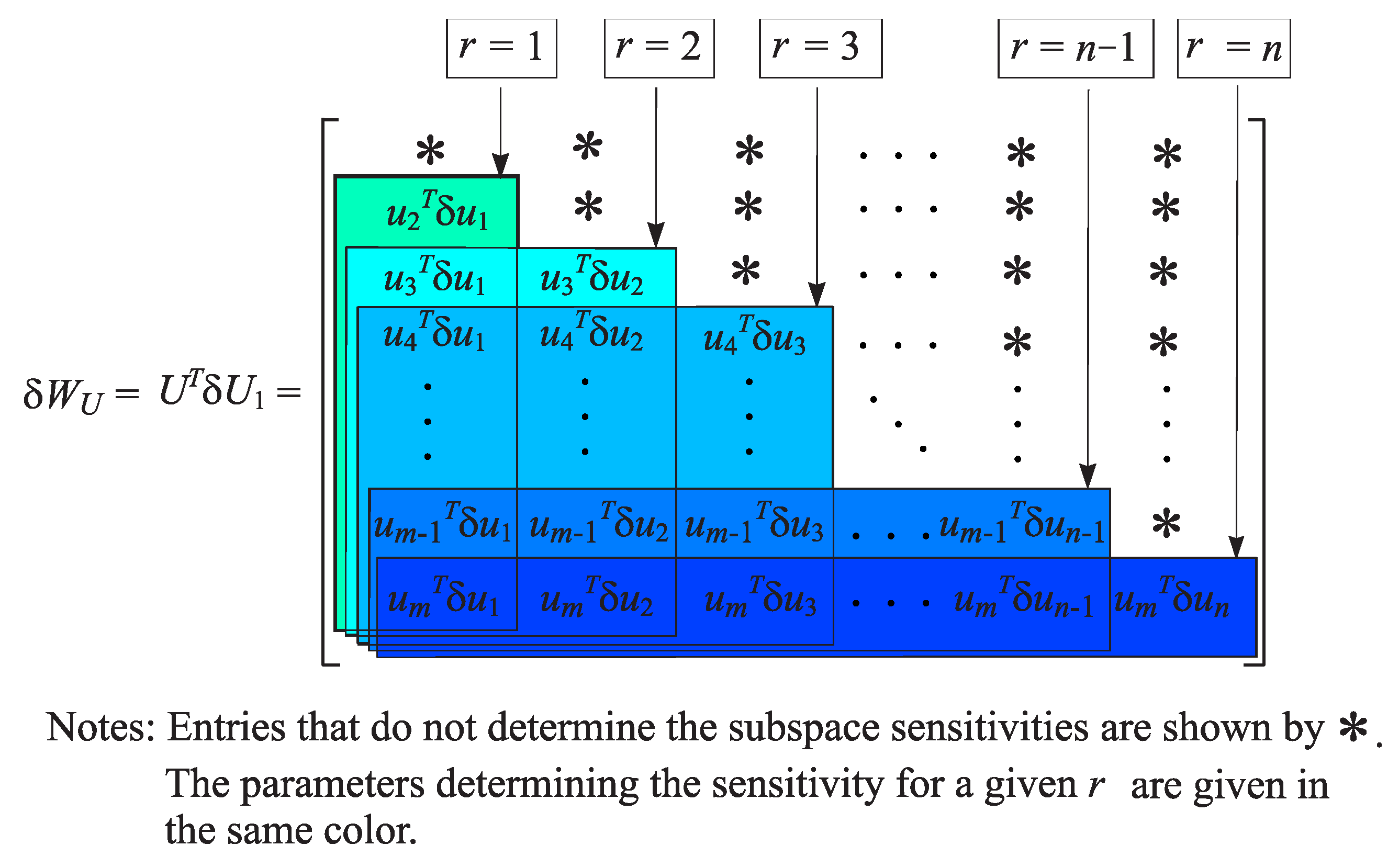
Equation (46) shows that the sensitivity of the left singular subspace ${\mathcal{U}}_r$ is related to the values of the perturbation parameters $x_k=u_i^T\delta u_j,k=i+(j-1)m-\frac{j(j+1)}{2},i>r,$$j=1,2,\dots ,r$. In particular, for $r=1$, the sensitivity of the first column of U (the left singular vector, corresponding to ${\sigma }_1$) is determined by

$$sin(\Phi \max ({\mathcal{U}}_1,{\tilde{\mathcal{U}}}_1))={\sigma }_{\max }(\delta {W_U}_{2:m,1}),$$

for $r=2$ one has

$$sin(\Phi \max ({\mathcal{U}}_2,{\tilde{\mathcal{U}}}_2))={\sigma }_{\max }(\delta {W_U}_{3:m,1:2})$$

and so on (see Figure 1), where the matrices ${U_{(r)}^{\perp }}^T\delta U_{(r)}=\delta {W_U}_{r+1:m,1:r}$ for different values of r are highlighted in boxes.

Figure 1. Sensitivity estimations of the left singular subspaces.

Similarly, utilizing the matrix $\delta W_V$, it is possible to find the sine of the maximum angle between the unperturbed ${\mathcal{V}}_r$ and the perturbed ${\tilde{\mathcal{V}}}_r$ right singular subspace

$$sin(\Theta \max ({\mathcal{V}}_r,\widetilde{{\mathcal{V}}_r}))={\sigma }_{\max }(\delta {W_V}_{r+1:n,1:r})$$

(see Figure 2). Hence, if the perturbation parameters are determined, it is possible to find sensitivity estimates of the nested singular subspaces

$$\begin{array}{ccc}\hfill {\mathcal{U}}_1=\mathrm{span}(U_{(1)})& =& \mathrm{span}(u_1),\hfill \\ \hfill {\mathcal{U}}_2=\mathrm{span}(U_{(2)})& =& \mathrm{span}(u_1,u_2),\hfill \\ \hfill ⋮& & ⋮\hfill \\ \hfill {\mathcal{U}}_r=\mathrm{span}(U_{(r)})& =& \mathrm{span}(u_1,u_2,\dots ,u_r),r=min\{m-1,n\}\hfill \end{array}$$

and

$$\begin{array}{ccc}\hfill {\mathcal{V}}_1=\mathrm{span}(V_{(1)})& =& \mathrm{span}(v_1),\hfill \\ \hfill {\mathcal{V}}_2=\mathrm{span}(V_{(2)})& =& \mathrm{span}(v_1,v_2),\hfill \\ \hfill ⋮& & ⋮\hfill \\ \hfill {\mathcal{V}}_{n-1}=\mathrm{span}(V_{(n)})& =& \mathrm{span}(v_1,v_2,\dots ,v_{n-1}).\hfill \end{array}$$

Figure 2. Sensitivity estimations of the right singular subspaces.

Specifically, as

$$\delta W_U=\left[\begin{array}{ccccc}*& *& *& \dots & *\\ x_1& *& *& \dots & *\\ x_2& x_m& *& \dots & *\\ ⋮& ⋮& ⋮& \ddots & ⋮\\ x_{n-1}& x_{m+n-3}& x_{2m+n-6}& \dots & *\\ ⋮& ⋮& ⋮& ⋮& ⋮\\ x_{m-1}& x_{2m-3}& x_{3m-6}& \dots & x_p\end{array}\right]\in {\mathbb{R}}^{m\times n},$$

we have that the exact maximum angle between the unperturbed and perturbed left singular subspace of dimension r is given by

$$\Phi \max ({\mathcal{U}}_r,{\tilde{\mathcal{U}}}_r)=arcsin({\sigma }_{\max }(\delta {W_U}_{r+1:m,1:r})).$$

(47)

Similarly, the maximum angle between the unperturbed and perturbed right singular subspace of dimension r is

$$\Theta \max ({\mathcal{V}}_r,{\tilde{\mathcal{V}}}_r)=arcsin({\sigma }_{\max }(\delta {W_V}_{r+1:m,1:r})).$$

(48)

Thus, we obtain the following result.

Theorem 3.

The asymptotic estimate of the angle $\Phi \max ({\mathcal{U}}_r,{\tilde{\mathcal{U}}}_r)$ between the unperturbed and perturbed singular subspace of dimension r satisfies

$$\begin{array}{ccc}\hfill |\Phi \max ({\mathcal{U}}_r,{\tilde{\mathcal{U}}}_r)|& \le & {\Phi \max }^{lin}({\mathcal{U}}_r,{\tilde{\mathcal{U}}}_r),\hfill \\ \hfill {\Phi \max }^{lin}({\mathcal{U}}_r,{\tilde{\mathcal{U}}}_r)& =& arcsin(\parallel \delta {W_U}_{r+1:m,1:r}^{lin}{\parallel }_2),\hfill \end{array}$$

(49)

where

$$\delta W_U^{lin}=\left[\begin{array}{ccccc}0& *& *& \dots & *\\ x_1^{lin}& 0& *& \dots & *\\ x_2^{lin}& x_m^{lin}& 0& \dots & *\\ ⋮& ⋮& ⋮& \ddots & ⋮\\ x_{n-1}^{lin}& x_{m+n-3}^{lin}& x_{2m+n-6}^{lin}& \dots & 0\\ ⋮& ⋮& ⋮& ⋮& ⋮\\ x_{m-1}^{lin}& x_{2m-3}^{lin}& x_{3m-6}^{lin}& \dots & x_p^{lin}\end{array}\right]\in {\mathbb{R}}^{m\times n}$$

and the parameters $x_k^{lin},k=1,2,\dots ,p$ are determined from (39).

In particular, for the sensitivity of the range $\mathcal{R}(A)$ of A, we obtain that

$$sin({\Phi \max }^{lin}({\mathcal{U}}_n,{\tilde{\mathcal{U}}}_n))={\parallel \delta {W_U}_{n+1:m,1:n}^{lin}\parallel }_2.$$

Similarly, for the angles between the unperturbed and perturbed right singular subspaces of dimension r, we obtain the linear estimates

$$\begin{array}{ccc}\hfill |\Theta \max ({\mathcal{V}}_r,{\tilde{\mathcal{V}}}_r)|& \le & {\Theta \max }^{lin}({\mathcal{U}}_r,{\tilde{\mathcal{U}}}_r),\hfill \\ \hfill {\Theta \max }^{lin}({\mathcal{V}}_r,{\tilde{\mathcal{V}}}_r)& =& arcsin(\parallel \delta {W_V}_{r+1:n,1:r}^{lin}{\parallel }_2),\hfill \end{array}$$

(50)

where

$$\delta W_V^{lin}=\left[\begin{array}{ccccc}0& *& *& \dots & *\\ y_1^{lin}& 0& *& \dots & *\\ y_2^{lin}& y_n^{lin}& 0& \dots & *\\ ⋮& ⋮& ⋮& \ddots & ⋮\\ y_{n-1}^{lin}& y_{2n-3}^{lin}& y_{3n-6}^{lin}& \dots & 0\end{array}\right]\in {\mathbb{R}}^{n\times n}$$

and $y_{\ell },\ell =1,2,\dots ,q$ are determined from (37).

We note that using separate x and y parameters decouples the SVD perturbation problem and makes it possible to determine the sensitivity estimates of the left and right singular subspaces independently. This is important when the left or right subspace in a pair of singular subspaces is much more sensitive than its counterpart.

Consider as an example the same perturbed matrix A as in Example 1. Computing the matrices $\delta W_U^{lin}$ and $\delta W_V^{lin}$, it is possible to estimate the sensitivity of all four pairs of singular subspaces of dimensions $r=1,2,3$, and 4 corresponding to the chosen ordering of the singular values. In Table 4, we show the actual values of the left and right singular subspaces sensitivity and the computed asymptotic estimates (49) and (50) of this sensitivity. To determine the sensitivity of other singular subspaces, reordering the singular values in the initial decomposition so that the desired subspace appears in the set of nested singular subspaces is possible. Note that asymptotic estimates of the canonical angles between an arbitrary unperturbed singular subspace ${\mathcal{U}}_q,q\le min\{m-1,n\}$ spanned by specific singular vectors combined in the matrix $U_q$ and its perturbed counterpart can be determined by computing the singular values of the matrix ${{U_q}^{\perp }}^T\delta U_q^{lin}$, where $U_q^{\perp }$ is the orthogonal complement of $U_q$, consisting of all singular vectors that do not participate in $U_q$, and $\delta U_q^{lin}$ is the linear estimate obtained by using (42). Similarly, it is possible to obtain asymptotic perturbation bounds for a desired right singular subspace.

Table 4. Sensitivity of the singular subspaces.

c	${\parallel \mathit{\delta }\mathit{A}\parallel }_2$	$|\mathbf{\Phi }\max ({\mathcal{U}}_{\mathit{r}},{\tilde{\mathcal{U}}}_{\mathit{r}})|$	$\mathbf{\Phi }{\mathbf{max}}^{\mathit{lin}}({\mathcal{U}}_{\mathit{r}},{\tilde{\mathcal{U}}}_{\mathit{r}})$
$-10$	$2.0819813\times {10}^{-9}$	${\Phi }_1=0.0024212\times {10}^{-8}$	${\Phi }_1=0.0002029\times {10}^{-6}$
		${\Phi }_2=0.0082136\times {10}^{-8}$	${\Phi }_2=0.0005938\times {10}^{-6}$
		${\Phi }_3=0.0103290\times {10}^{-7}$	${\Phi }_3=0.0029428\times {10}^{-6}$
		${\Phi }_4=0.1074643\times {10}^{-7}$	${\Phi }_4=0.1662787\times {10}^{-6}$
$-5$	$2.0819812\times {10}^{-4}$	${\Phi }_1=0.0024212\times {10}^{-3}$	${\Phi }_1=0.0020294\times {10}^{-2}$
		${\Phi }_2=0.0082136\times {10}^{-3}$	${\Phi }_2=0.0059380\times {10}^{-2}$
		${\Phi }_3=0.1032951\times {10}^{-3}$	${\Phi }_3=0.0294279\times {10}^{-2}$
		${\Phi }_4=0.1073496\times {10}^{-2}$	${\Phi }_4=1.6628641\times {10}^{-2}$
$\mathbf{c}$	${\parallel \mathbf{\delta }\mathbf{A}\parallel }_{\mathbf{2}}$	$|\Theta \mathbf{max}({\mathcal{V}}_{\mathbf{r}},{\tilde{\mathcal{V}}}_{\mathbf{r}})|$	$\Theta {\mathbf{max}}^{\mathit{lin}}({\mathcal{V}}_{\mathbf{r}},{\tilde{\mathcal{V}}}_{\mathbf{r}})$
$-10$	$2.0819813\times {10}^{-9}$	${\Theta }_1=0.0425801\times {10}^{-9}$	${\Theta }_1=0.0166760\times {10}^{-8}$
		${\Theta }_2=0.0438355\times {10}^{-9}$	${\Theta }_2=0.0438688\times {10}^{-8}$
		${\Theta }_3=0.2782232\times {10}^{-9}$	${\Theta }_3=0.1714819\times {10}^{-8}$
$-5$	$2.0819812\times {10}^{-4}$	${\Theta }_1=0.0425804\times {10}^{-4}$	${\Theta }_1=0.0166760\times {10}^{-3}$
		${\Theta }_2=0.0438356\times {10}^{-4}$	${\Theta }_2=0.0438688\times {10}^{-3}$
		${\Theta }_3=0.2782378\times {10}^{-4}$	${\Theta }_3=0.1714819\times {10}^{-3}$

9. Global Perturbation Bounds

Since analytical expressions for the global perturbation bounds of the singular value decompositions are unknown up to this moment, we present an iterative procedure for finding estimates of these bounds based on the asymptotic analysis presented above. This procedure is similar to the corresponding iterative schemes proposed in [26] but is more complicated since determining bounds on the parameter vectors x and y must be performed simultaneously because the equations for these parameters are coupled.

9.1. Perturbation Bounds of the Entries of $U_2$

The main difficulty in determining global bounds of x and y is to find an appropriate approximation of the high-order term ${\Delta }_2$ in (23). As is seen from (25), the determining of such an estimate requires knowing the perturbation $\delta U_2$, which is not well determined since it contains the columns of the matrix $\delta U_2={\tilde{U}}_2-U_2$. This perturbation satisfies the equations

$$\begin{array}{ccc}\hfill {(U_1+\delta U_1)}^T(U_2+\delta U_2)& =& 0,\hfill \end{array}$$

(51)

$$\begin{array}{ccc}\hfill {(U_2+\delta U_2)}^T(U_2+\delta U_2)& =& I_{m-n}\hfill \end{array}$$

(52)

which follow from the orthogonality of the matrix

$$\tilde{U}=[U_1+\delta U_1,U_2+\delta U_2].$$

An estimate of $\delta U_2$ can be found based on a suitable approximation of

$$X=U^T\delta U_2:=\left[\begin{array}{c}{X}_1\\ X_2\end{array}\right].$$

As shown in [26], a first-order approximation of the matrix X can be determined using the estimates

$$\begin{array}{ccc}\hfill X_1^{appr}& =& -{(I_n+\delta W_1^T)}^{-1}\delta W_2^T\in {\mathbb{R}}^{n\times (m-n)},\hfill \end{array}$$

(53)

$$\begin{array}{ccc}\hfill X_2^{appr}& =& -{X_1^{appr}}^T{X}_1^{appr}/2\in {\mathbb{R}}^{(m-n)\times (m-n)},\hfill \end{array}$$

(54)

where $\delta W_1=U_1^T\delta U_1$, $\delta W_2=U_2^T\delta U_1$ and for sufficiently small perturbation $\delta U_1$, the matrix $I_n+\delta W_1^T$ is nonsingular. (Note that $\delta W_U={\left[\delta W_1^T\delta W_2^T\right]}^T$ is already estimated.) Thus, we have that

$$\delta U_2^{appr}=U{X}^{appr}.$$

(55)

9.2. Iterative Procedure for Finding Global Bounds of x and y

Global componentwise perturbation bounds of the matrices U and V can be found using nonlinear estimates of the matrices $\delta W_U$ and $\delta W_V$, determined by (15) and (16), respectively. Such estimates are found correcting the linear estimates of the perturbation parameters $x_k=u_i^T\delta u_j$ and $y_{\ell }=v_i^T\delta v_j$ on each iteration step. This approach is used in [9,32] (Ch. 4), and [33] in the normwise perturbation analysis of invariant subspaces and is related to the solution of the nonlinear equation

$$\mathbf{T}x=g-\varphi (x),$$

where $\mathbf{T}$ is a linear operator corresponding to the asymptotic perturbation estimate and $\varphi (x)$ reflects the higher order terms corresponding to the nonlinear correction of the estimate. In finding the normwise global perturbation bounds, the above operator equation can be solved analytically using the contraction mapping theorem. Unfortunately, in the determining of componentwise estimates it is necessary to solve a system of complicated nonlinear equations and in such case the determining of analytical nonlinear bounds is difficult. That is why, in finding global bounds, we shall implement an iterative technique, similar to the one presented in [26]. Like the asymptotic estimates, the global bounds can be found only knowing the norm of $\delta A$. This is performed approximating in the best possible way the higher-order terms (15) and (16), using on each step the approximations of the parameter vectors x and y. We note that the iteration convergence is established only experimentally, and the derivation of a convergence proof is a matter for further investigation. Thus, the proposed iterative procedure should be considered only as an illustrative one.

Consider the case of estimating the matrix $\delta W_U$. It is convenient to substitute the terms containing the perturbations $\delta u_j$ in (15) with the quantities

$$\delta {w_u}_j=U^T\delta u_j,j=1,2,\dots ,n,$$

which have the same magnitude as $\delta u_j$. Since

$$\delta u_i^T\delta u_j=\delta u_i^{T}U{U}^T\delta u_j=\delta {w_u}_i^T\delta {w_u}_j,$$

the absolute value of the matrix $\delta W_U\in {\mathbb{R}}^{m\times n}$ (15) can be bounded as

$$\begin{array}{ccc}\hfill |\delta W_U^{nonl}|& =& |U^T\delta U_1|=\left[\right|\delta {w_u}_1|,|\delta {w_u}_2|,\dots ,|\delta {w_u}_n\left|\right]\hfill \\ & ⪯& |\delta Q_U|+|\delta D_U|+|\delta N_U|,\hfill \end{array}$$

(56)

where

The diagonal entries $\delta {d_u}_{jj},j=1,2,\dots ,n$ can be found from the entries of $\delta Q_U$ by using the approximation (14). Since the unknown column estimates $|\delta w_j|$ participate in both sides of (56), it is possible to obtain them as follows. The first column of $\delta W_U$ is determined from

$$|\delta {w_u}_1|=|\delta {q_u}_1|+|\delta {d_u}_1|,$$

where $|\delta {q_u}_1|$, $|\delta d_1|$ are the first columns of $|\delta Q_U|$, $|\delta D_U|$, respectively. Then, the next column estimates $|\delta w_j|,j=2,3,\dots n$ can be determined recursively from

$$|\delta {w_u}_j|=|\delta {q_u}_j|+|\delta {d_u}_j|+\left[\begin{array}{c}|\delta {w_u}_1^T\left|\right|\delta {w_u}_j|\\ |\delta {w_u}_2^T\left|\right|\delta {w_u}_j|\\ ⋮\\ |\delta {w_u}_{j-1}^T\left|\right|\delta {w_u}_j|\\ 0\\ ⋮\\ 0\end{array}\right],$$

which is equivalent to solving the linear system

$$|{S_U}_j\left|\right|\delta {w_u}_j|=|\delta {q_u}_j|+|\delta {d_u}_j|,$$

where

$$|{S_U}_j|=\left[\begin{array}{c}{e}_1^T-\left|\delta {w_u}_1^T\right|\\ e_2^T-\left|\delta {w_u}_2^T\right|\\ ⋮\\ e_{j-1}^T-\left|\delta {w_u}_{j-1}^T\right|\\ e_j^T\\ ⋮\\ e_n^T\end{array}\right]\in {\mathbb{R}}^{m\times m}$$

and $e_j$ is the jth column of $I_m$. The matrix $|{S_U}_j|$ is upper triangular with unit diagonal and if $|\delta {w_u}_i|,i=1,2,\dots ,j-1$ have small norms, then the matrix $|{S_U}_j|$ is diagonally dominant. Hence, it is very well conditioned with a condition number close to 1.

As a result we obtain that

$$\left|\delta {w_u}_j\right|⪯|{S_U}_j{|}^{-1}(|\delta {q_u}_j|+|\delta {d_u}_j|)$$

(57)

which produces the jth column of $|\delta W_U^{nonl}|$.

A similar recursive procedure can be used to determine the quantities $|\delta {w_v}_j|=|v_i^T\delta v_j|$. In this case for each j it is necessary to solve the nth order linear system

$$\left|{S_V}_j\right|\left|\delta {w_v}_j\right|=|\delta {q_v}_j|+|\delta {d_v}_j|.$$

The estimates of $|\delta {w_u}_j|,j=1,2,\dots ,m$ and $|\delta {w_v}_j|,j=1,2,\dots ,n$ thus obtained, are used to bound the absolute values of the nonlinear elements ${\Delta }_1$ and ${\Delta }_2$ given in (24) and (25), respectively. Utilizing the approximation of $U^T\delta U_2$, it is possible to find an approximation of the matrix $U^T\delta U$ as

$$Z=[\delta W_U^{nonl},\delta U_2^{appr}]:=[Z_1,Z_2],Z_1\in {\mathbb{R}}^{m\times n},Z_2\in {\mathbb{R}}^{m\times (m-n)}$$

where $\delta U_2^{appr}=U{X}^{appr}$,

$$X^{appr}=\left[\begin{array}{c}{X}_1^{appr}\\ X_2^{appr}\end{array}\right]$$

and $X_1^{appr},X_2^{appr}$ are given by (53), (54). Then, the elements of ${\Delta }_1$, ${\Delta }_2$ are bounded according to (24) and (25) as

$$\begin{array}{ccc}\hfill |{{\Delta }_1}_{ij}^{nonl}|& \le & {\sigma }_j|{Z_1}_i{|}^T|{Z_1}_j|+|{Z_1}_i{|}^T\Sigma \left|Y_j\right|+\hfill \\ & & (\parallel {Z_1}_i{\parallel }_2+\parallel Y_j{\parallel }_2+\parallel {Z_1}_i{\parallel }_2\parallel Y_j{\parallel }_2{)\parallel \delta A\parallel }_2,\hfill \\ & & i=1,2,\dots ,n,j=1,2,\dots ,n,\hfill \end{array}$$

(58)

$$\begin{array}{ccc}\hfill |{{\Delta }_2}_{ij}^{nonl}|& \le & {\sigma }_j|{Z_2}_i{|}^T|{Z_1}_j|+|{Z_2}_i{|}^T\Sigma \left|Y_j\right|+\hfill \\ & & (\parallel {Z_2}_i{\parallel }_2+\parallel Y_j{\parallel }_2+\parallel {Z_2}_i{\parallel }_2\parallel Y_j{\parallel }_2{)\parallel \delta A\parallel }_2.\hfill \\ & & i=1,2,\dots ,m-n,j=1,2,\dots ,n.\hfill \end{array}$$

(59)

Utilizing (31) and (32), the nonlinear corrections of the vectors $x_{(1)}$ and y can be determined from

$$\begin{array}{ccc}\hfill \delta x_{(1)}& =& |S_{xf}|\mathrm{vec}(\mathrm{Low}(|{\Delta }_1|)+|S_{xg}|\mathrm{vec}((\mathrm{Up}(|\delta {N_U}_1|{\Sigma }_n\hfill \\ & & +{\Sigma }_n|\delta N_V|+|{\Delta }_1^{nonl}{|))}^T),\hfill \end{array}$$

(60)

$$\begin{array}{ccc}\hfill \delta y& =& |S_{yf}|\mathrm{vec}(\mathrm{Low}(|{\Delta }_1|)+|S_{yg}|\mathrm{vec}((\mathrm{Up}(|\delta {N_U}_1|{\Sigma }_n\hfill \\ & & +{\Sigma }_n|\delta N_V|+|{\Delta }_1{|}^{nonl}{))}^T),\hfill \end{array}$$

(61)

where $|\delta {N_U}_1|$ is estimated by using the corresponding expression (56) and $|\delta N_V|$—is estimated by using a similar expression.

The nonlinear correction of $x_{(2)}$ is found from

$$\begin{array}{ccc}\hfill \delta x_{(2)}& =& \mathrm{vec}(Z),\hfill \\ \hfill Z& =& \parallel {\Delta }_2^{nonl}{\parallel }_2\times \left[\begin{array}{cccc}1/{\sigma }_1& 1/{\sigma }_2& \dots & 1/{\sigma }_n\\ 1/{\sigma }_1& 1/{\sigma }_2& \dots & 1/{\sigma }_n\\ ⋮& ⋮& ⋮& ⋮\\ 1/{\sigma }_1& 1/{\sigma }_2& \dots & 1/{\sigma }_n\end{array}\right].\hfill \end{array}$$

(62)

and the total correction vector is determined from

$$\delta x={\Omega }_1^T\delta x_{(1)}+{\Omega }_2^T\delta x_{(2)}.$$

(63)

Now, the nonlinear estimates of the vectors x and y are found from

$$\begin{array}{ccc}\hfill x^{nonl}& =& x^{lin}+\delta x,\hfill \end{array}$$

(64)

$$\begin{array}{ccc}\hfill y^{nonl}& =& y^{lin}+\delta y.\hfill \end{array}$$

(65)

In this way, we obtain an iterative scheme for finding simultaneously nonlinear estimates of the coupled perturbation parameter vectors x and y involving the Equations (56)–(59) and (60)–(65). In the numerical experiments presented below, the initial conditions are chosen as $x_0^{nonl}=eps{[1,1,\dots ,1]}^T$ and $y_0^{nonl}=eps{[1,1,\dots ,1]}^T$, where $eps$ is the MATLAB^®function eps, $eps=2^{-52}$. The stopping criteria for x- and y-iterations are taken as

$$\begin{array}{ccc}\hfill er{r}_x& =& {\parallel x_s^{nonl}-x_{s-1}^{nonl}\parallel }_2/{\parallel x_{s-1}^{nonl}\parallel }_2<tol,\hfill \\ \hfill er{r}_y& =& {\parallel y_s^{nonl}-y_{s-1}^{nonl}\parallel }_2/{\parallel y_{s-1}^{nonl}\parallel }_2<tol,\hfill \end{array}$$

where $tol=10eps$. The scheme converges for perturbations $\delta A$ of restricted size. It is possible that y converges while x does not converge.

The nonlinear estimate of the higher term ${\Delta }_1$ can be used to obtain nonlinear corrections of the singular value perturbations. Based on (40), a nonlinear correction of each singular value can be determined as

$$\delta {\sigma }_i^{corr}=(|\delta {D_U}_1|{\Sigma }_n+{\Sigma }_n|\delta D_V|+|{\Delta }_1{|)}_{ii},$$

(66)

so that the corresponding singular value perturbation is estimated as

$$\delta {\sigma }_i^{nonl}={\sigma }_i^{lin}+\delta {\sigma }_i^{corr}.$$

Note that ${\sigma }_i^{lin}=\left|\delta f_{ii}\right|$ is known only when the entries of the perturbation $\delta A$ are known, and usually, this is not fulfilled in practice. Nevertheless, the nonlinear correction (66) can be useful in estimating the sensitivity of a given singular value.

In Table 5, we present the number of iterations necessary to find the global bound $x^{nonl}$ for the problem considered in Example 1 with perturbations $\delta A={10}^c\times A_0,c=-10,-9,\dots ,-3$. In the last two columns of the table, we give the norm of the exact higher-order term $\Delta$ and its approximation $\parallel {\Delta }^{nonl}{\parallel }_2$ computed according to (58) and (59) (the approximation is given for the last iteration). In particular, for the perturbation $\delta A={10}^{-5}{A}_0$, the exact higher-order term $\Delta$, found using (24) and (25), is

$$\begin{array}{ccc}\hfill |\Delta |& =& {10}^{-7}\times \left[\begin{array}{cccc}0.0045563& 0.0006839& 0.0146195& 0.0257942\\ 0.0012737& 0.0008692& 0.0080543& 0.0003708\\ 0.0000993& 0.0015257& 0.0086067& 0.0085598\\ 0.0019107& 0.0007767& 0.0258012& 0.0170781\\ 0.0032494& 0.0006701& 0.0423789& 0.2046100\\ 0.0064032& 0.0004567& 0.0384765& 0.0071094\end{array}\right],\hfill \\ \hfill {\parallel \Delta \parallel }_2& =& 2.12746\times {10}^{-8}.\hfill \end{array}$$

Table 5. Convergence of the global bounds and higher-order terms.

c	${\parallel \mathit{\delta }\mathit{A}\parallel }_{\mathit{F}}$	Number of Iterations	${\parallel \mathit{\Delta }\parallel }_2$	$\parallel {\mathit{\Delta }}^{\mathit{nonl}}{\parallel }_2$
$-10$	$2.08198\times {10}^{-9}$	4	$2.12806\times {10}^{-18}$	$2.09530\times {10}^{-15}$
$-9$	$2.08198\times {10}^{-8}$	4	$2.12806\times {10}^{-16}$	$2.09531\times {10}^{-13}$
$-8$	$2.08198\times {10}^{-7}$	5	$2.12806\times {10}^{-14}$	$2.09537\times {10}^{-11}$
$-7$	$2.08198\times {10}^{-6}$	5	$2.12806\times {10}^{-12}$	$2.09595\times {10}^{-9}$
$-6$	$2.08198\times {10}^{-5}$	7	$2.12800\times {10}^{-10}$	$2.10185\times {10}^{-7}$
$-5$	$2.08198\times {10}^{-4}$	10	$2.12746\times {10}^{-8}$	$2.16338\times {10}^{-5}$
$-4$	$2.08198\times {10}^{-3}$	29	$2.12189\times {10}^{-6}$	$3.23896\times {10}^{-3}$
$-3$	$2.08198\times {10}^{-2}$	No convergence	-	-

Implementing the described iterative procedure, after 10 iterations, we obtain the nonlinear bound

$$\begin{array}{ccc}\hfill {\Delta }^{nonl}& =& {10}^{-5}\times \left[\begin{array}{cccc}0.0019716& 0.0021343& 0.0049111& 0.0047911\\ 0.0041273& 0.0053422& 0.0069174& 0.0069309\\ 0.0189857& 0.0186412& 0.0222135& 0.0179503\\ 0.8671799& 0.8680880& 0.8664831& 0.8607933\\ 0.5146400& 0.5162827& 0.5207565& 0.2618103\\ 0.5146400& 0.5162827& 0.5207565& 0.2618103\end{array}\right],\hfill \\ \hfill \parallel {\Delta }^{nonl}{\parallel }_2& =& 2.16338\times {10}^{-5}\hfill \end{array}$$

computed according to (58) and (59) on the base of the nonlinear bound $x^{nonl}$.

The global bounds $\parallel x^{nonl}{\parallel }_2$ and $\parallel y^{nonl}{\parallel }_2$, found for different perturbations along with the values of ${\parallel x\parallel }_2$ and ${\parallel y\parallel }_2$, are shown in Table 6. The results confirm that the global estimates of x and y are close to the corresponding asymptotic estimates.

Table 6. Global bounds of x and y.

c	${\parallel \mathit{x}\parallel }_2$	$\parallel {\mathit{x}}^{\mathit{nonl}}{\parallel }_2$	${\parallel \mathit{y}\parallel }_2$	$\parallel {\mathit{y}}^{\mathit{nonl}}{\parallel }_2$
$-10$	$1.0782203\times {10}^{-8}$	$1.6628799\times {10}^{-7}$	$2.8118399\times {10}^{-10}$	$1.7511069\times {10}^{-9}$
$-9$	$1.0782176\times {10}^{-7}$	$1.6628817\times {10}^{-6}$	$2.8118379\times {10}^{-9}$	$1.7511072\times {10}^{-8}$
$-8$	$1.0782167\times {10}^{-6}$	$1.6628999\times {10}^{-5}$	$2.8118393\times {10}^{-8}$	$1.7511098\times {10}^{-7}$
$-7$	$1.0782065\times {10}^{-5}$	$1.6630816\times {10}^{-4}$	$2.8118405\times {10}^{-7}$	$1.7511358\times {10}^{-6}$
$-6$	$1.0781037\times {10}^{-4}$	$1.6649057\times {10}^{-3}$	$2.8118536\times {10}^{-6}$	$1.7513967\times {10}^{-5}$
$-5$	$1.0770771\times {10}^{-3}$	$1.6837998\times {10}^{-2}$	$2.8119844\times {10}^{-5}$	$1.7540888\times {10}^{-4}$
$-4$	$1.0668478\times {10}^{-2}$	$1.9743124\times {10}^{-1}$	$2.8132907\times {10}^{-4}$	$1.7960922\times {10}^{-3}$

In Figure 3 and Figure 4, we show the convergence of the relative errors

$$er{r}_x=\parallel x_s^{nonl}-x_{s-1}^{nonl}\parallel /\parallel x_{s-1}^{nonl}\parallel$$

and

$$er{r}_y=\parallel y_s^{nonl}-y_{s-1}^{nonl}\parallel /\parallel y_{s-1}^{nonl}\parallel ,$$

respectively, at step s of the iterative process for different perturbations $\delta A={10}^c\times A_0$. (The value of the relative error on each step is shown by a circle.) As it is seen from the figures, for the given example the convergence of y is close to the convergence of x. For all values of c, except $c=-3$, the relative error begins with values $er{r}_x,er{r}_y>>1$ and ends with values $er{r}_x,er{r}_y<{10}^{-13}$. With the increasing in the perturbation size, the convergence becomes slower and for $c=-3$$(\parallel \delta A{\parallel }_2=2.08198\times {10}^{-2})$, the iteration diverges. This demonstrates the restricted usefulness of the nonlinear estimates, which is valid only for limited perturbation magnitudes.

Figure 3. Relative errors in the iterative determining of the global bounds of x.

Figure 4. Relative errors in the iterative determining of the global bounds of y.

In Table 7, we give normwise perturbation bounds of the singular values along with the actual singular value perturbations and their global bounds found for two perturbations of A under the assumption that the linear bounds of all singular values are known. As can be seen from the table, the nonlinear estimates of the singular values are very tight.

Table 7. Perturbations of the singular values and their nonlinear estimates.

c	$\mathit{\delta }{\widehat{\mathit{\sigma }}}_{\mathit{i}}={\parallel \mathit{\delta }\mathit{A}\parallel }_2$	$|\mathit{\delta }{\mathit{\sigma }}_{\mathit{i}}|$	$\mathit{\delta }{\mathit{\sigma }}_{\mathit{i}}^{\mathit{nonl}}$
$-10$	$2.0819812\times {10}^{-9}$	$\delta {\sigma }_1=0.1543977\times {10}^{-8}$	$\delta {\sigma }_1=0.1543978\times {10}^{-8}$
		$\delta {\sigma }_2=0.4299672\times {10}^{-10}$	$\delta {\sigma }_2=0.4299589\times {10}^{-10}$
		$\delta {\sigma }_3=0.6114032\times {10}^{-9}$	$\delta {\sigma }_3=0.6114031\times {10}^{-9}$
		$\delta {\sigma }_4=0.1736317\times {10}^{-9}$	$\delta {\sigma }_4=0.1736329\times {10}^{-9}$
$-5$	$2.0819812\times {10}^{-4}$	$\delta {\sigma }_1=0.1543975\times {10}^{-3}$	$\delta {\sigma }_1=0.1544264\times {10}^{-3}$
		$\delta {\sigma }_2=0.4299891\times {10}^{-5}$	$\delta {\sigma }_2=0.4373954\times {10}^{-5}$
		$\delta {\sigma }_3=0.6113327\times {10}^{-4}$	$\delta {\sigma }_3=0.6143758\times {10}^{-4}$
		$\delta {\sigma }_4=0.1737508\times {10}^{-4}$	$\delta {\sigma }_4=0.2848085\times {10}^{-4}$

9.3. Global Perturbation Bounds of $\delta U_1$ and $\delta V$

Having nonlinear bounds of x, y, $|\delta W_U|$, and $|\delta W_V|$, we may find nonlinear bounds on the perturbations of the entries of $U_1$ and V according to the relationships

$$\begin{array}{ccc}\hfill \delta U_1^{nonl}& =& \left|U\right|\delta W_U^{nonl},\hfill \end{array}$$

(67)

$$\begin{array}{ccc}\hfill \delta V^{nonl}& =& \left|V\right|\delta W_V^{nonl}.\hfill \end{array}$$

(68)

For the perturbations of the orthogonal matrices of Example 1 in the case of $\delta A={10}^{-5}{A}_0$, we obtain the nonlinear componentwise bounds

$$\delta U_1^{nonl}={10}^{-2}\times \left[\begin{array}{cccc}0.0018797& 0.0053307& 0.0221710& 0.9714224\\ 0.0012678& 0.0045195& 0.0227162& 1.4182521\\ 0.0014492& 0.0046330& 0.0227031& 0.5447168\\ 0.0017643& 0.0042429& 0.0164150& 0.5441097\\ 0.0015182& 0.0034345& 0.0120243& 0.6452928\\ 0.0017076& 0.0051060& 0.0184868& 0.9697071\end{array}\right]$$

and

$$\delta V^{nonl}={10}^{-3}\times \left[\begin{array}{cccc}0.0110869& 0.0341506& 0.1618907& 0.0371700\\ 0.0130756& 0.0300673& 0.0179387& 0.1611512\\ 0.0161396& 0.0250967& 0.0804756& 0.1022096\\ 0.0056705& 0.0191966& 0.0673203& 0.0164507\end{array}\right].$$

These bounds are close to the obtained respective linear estimates $\delta U_1^{lin}$ and $\delta V^{lin}$ in Section 7.

Based on (47) and (48), global estimates of the maximum angles between the unperturbed and perturbed singular subspaces of dimension r can be obtained using the nonlinear bounds $\delta W_U^{nonl}$ and $\delta W_V^{nonl}$ of the matrices $\delta W_U$ and $\delta W_V$, respectively. For the pair of left and right singular subspaces of dimension r, we obtain that

$$\begin{array}{ccc}\hfill {\Phi \max }^{nonl}({\mathcal{U}}_r,{\tilde{\mathcal{U}}}_r)& =& arcsin(\parallel {\delta W_U}_{r+1:m,1:r}^{nonl}{\parallel }_2),\hfill \\ & & r\le min\{m-1,n\},\hfill \end{array}$$

(69)

$$\begin{array}{ccc}\hfill {\Theta \max }^{nonl}({\mathcal{V}}_r,{\tilde{\mathcal{V}}}_r)& =& arcsin(\parallel {\delta W_V}_{r+1:n,1:r}^{nonl}{\parallel }_2),\hfill \\ & & r\le n-1.\hfill \end{array}$$

(70)

In Table 8, we give the exact angles between the unperturbed and perturbed left and right singular subspaces of different dimensions and their nonlinear bounds computed using (69) and (70) for the matrix A from Example 1 and two perturbations $\delta A={10}^c\times A_0,c=-10,-5$. The comparison with the corresponding linear bounds in Table 4 shows that the two types of bounds produce close results. As in estimating the other elements of the singular value decomposition, the global perturbation bounds are slightly larger than the corresponding asymptotic estimates but give guaranteed bounds on the changes of the respective elements, although for a limited size of $\parallel \delta A\parallel$.

Table 8. Nonlinear sensitivity estimates of the singular subspaces.

c	${\parallel \mathit{\delta }\mathit{A}\parallel }_2$	$|\mathbf{\Phi }\max ({\mathcal{U}}_{\mathit{r}},{\tilde{\mathcal{U}}}_{\mathit{r}})|$	$\mathbf{\Phi }{\max }^{\mathit{nonl}}({\mathcal{U}}_{\mathit{r}},{\tilde{\mathcal{U}}}_{\mathit{r}})$
$-10$	$2.0819813\times {10}^{-9}$	${\Phi }_1=0.0024212\times {10}^{-8}$	${\Phi }_1=0.0002029\times {10}^{-6}$
		${\Phi }_2=0.0082136\times {10}^{-8}$	${\Phi }_2=0.0005938\times {10}^{-6}$
		${\Phi }_3=0.1032901\times {10}^{-8}$	${\Phi }_3=0.0029428\times {10}^{-6}$
		${\Phi }_4=1.0746434\times {10}^{-8}$	${\Phi }_4=0.1662788\times {10}^{-6}$
$-5$	$2.0819812\times {10}^{-4}$	${\Phi }_1=0.0024212\times {10}^{-3}$	${\Phi }_1=0.0020601\times {10}^{-2}$
		${\Phi }_2=0.0082136\times {10}^{-3}$	${\Phi }_2=0.0060635\times {10}^{-2}$
		${\Phi }_3=0.1032951\times {10}^{-3}$	${\Phi }_3=0.0303251\times {10}^{-2}$
		${\Phi }_4=1.0734956\times {10}^{-3}$	${\Phi }_4=1.6837810\times {10}^{-2}$
$\mathbf{c}$	${\parallel \mathbf{\delta }\mathbf{A}\parallel }_{\mathbf{2}}$	$|\Theta \mathbf{max}({\mathcal{V}}_{\mathbf{r}},{\tilde{\mathcal{V}}}_{\mathbf{r}})|$	$\Theta {\mathbf{max}}^{\mathit{nonl}}({\mathcal{V}}_{\mathbf{r}},{\tilde{\mathcal{V}}}_{\mathbf{r}})$
$-10$	$2.0819813\times {10}^{-9}$	${\Theta }_1=0.0425801\times {10}^{-9}$	${\Theta }_1=0.0166760\times {10}^{-8}$
		${\Theta }_2=0.0438355\times {10}^{-9}$	${\Theta }_2=0.0438688\times {10}^{-8}$
		${\Theta }_3=0.2782232\times {10}^{-9}$	${\Theta }_3=0.1714819\times {10}^{-8}$
$-5$	$2.0819812\times {10}^{-4}$	${\Theta }_1=0.0425804\times {10}^{-4}$	${\Theta }_1=0.0166819\times {10}^{-3}$
		${\Theta }_2=0.0438356\times {10}^{-4}$	${\Theta }_2=0.0438972\times {10}^{-3}$
		${\Theta }_3=0.2782378\times {10}^{-4}$	${\Theta }_3=0.1718211\times {10}^{-3}$

10. Numerical Experiments

In this section, we present the results of some numerical experiments illustrating the properties of the asymptotic and global estimates obtained in the paper. The computations are performed with MATLAB^®Version 9.9 (R2020b) [29] using IEEE double-precision arithmetic and are verified by using GNU Octave, v. 5.2.0. The M-files implementing the linear and nonlinear SVD perturbation estimates along the example files are available from the authors.

Example 2.

This example illustrates the ill-conditioning of the singular subspaces in the case of close singular values of the given matrix.

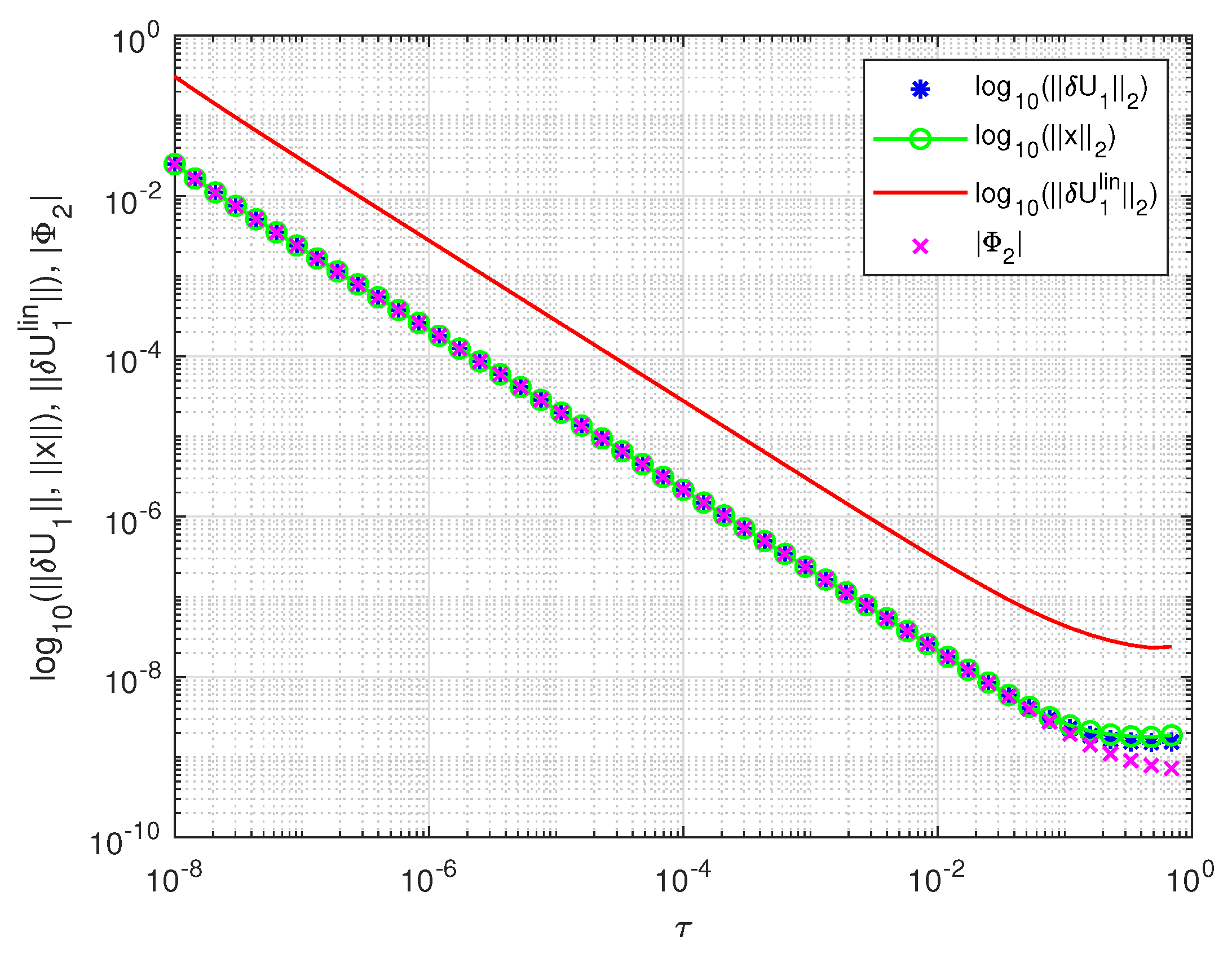
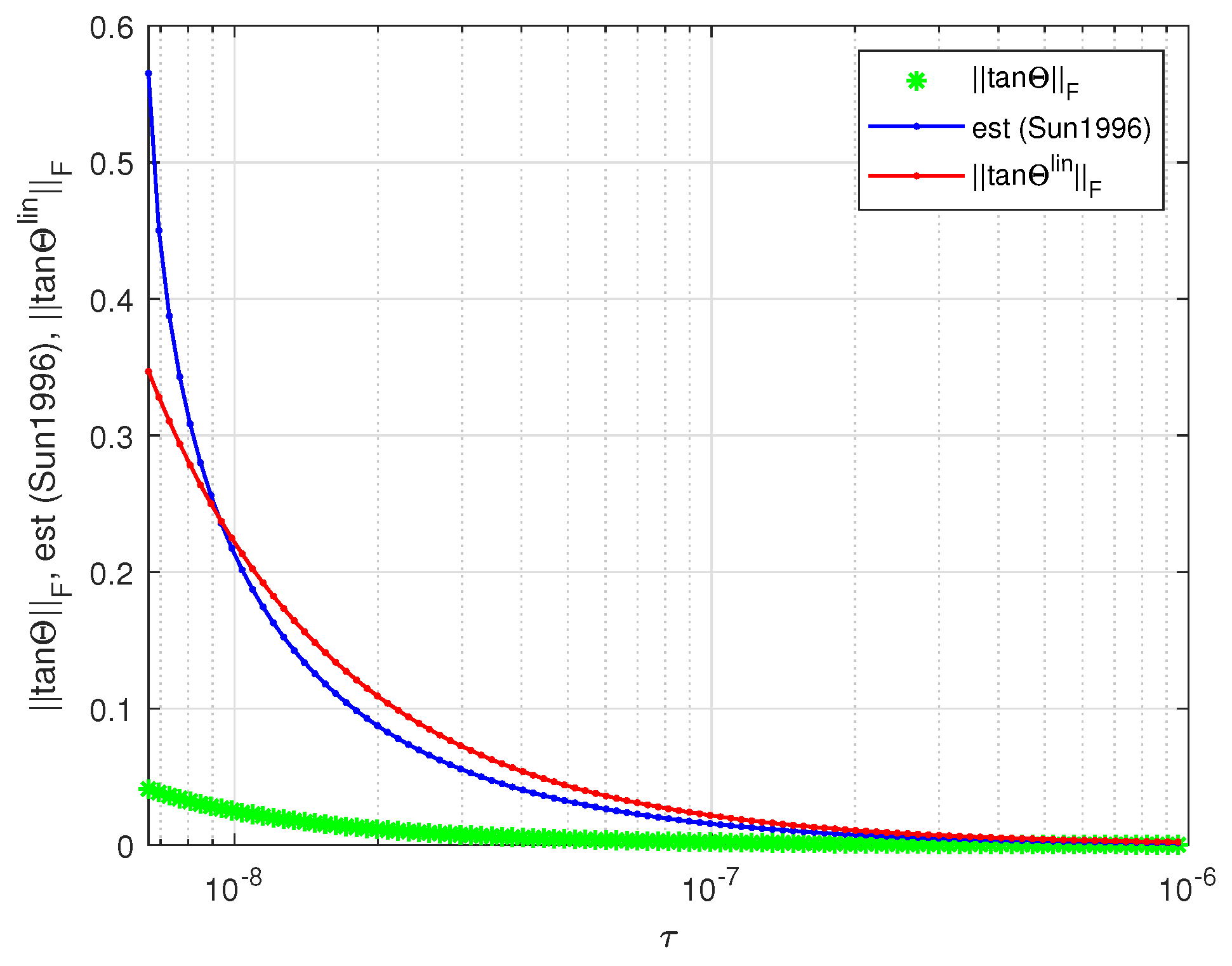
Consider a $10\times 3$ matrix A obtained as

$$A=U_0{\Sigma }_0{V}_0^T,$$

where

$$\begin{array}{ccc}\hfill U_0& =& I-2e{e}^T/10,e=[1,1,\dots ,1],\hfill \\ \hfill V_0& =& I-2h{h}^T/3,h=[1,-1,1]\hfill \end{array}$$

are orthogonal ad symmetric matrices (elementary reflections [Ch. 4] [2]) and

$$\mathrm{diag}({\Sigma }_0)=(2,1+\tau ,1),$$

where the parameter τ varies between ${10}^{-8}$ and ${10}^{-1}$.

In Figure 5, we present the actual values of $\parallel \delta U_1{\parallel }_2,{\parallel x\parallel }_2$ and the angle $|\Phi {\max }_2|$ along with the asymptotic normwise estimate $\parallel \delta U_1^{lin}{\parallel }_2$ as functions of the difference $\tau ={\sigma }_2-{\sigma }_3={10}^{-8},\dots ,{10}^{-1}$. Similarly, in Figure 6, we show the values of ${\parallel \delta V\parallel }_2,{\parallel y\parallel }_2$ and the angle $|\Theta {\max }_2|$ together with the asymptotic estimate $\parallel \delta V^{lin}{\parallel }_2$ as functions of τ. Note that $\Phi {\max }_2$ is the larger angle between the subspaces ${\mathcal{U}}_{(2)}=\mathrm{span}(u_1,u_2)$ and ${\tilde{\mathcal{U}}}_{(2)}=\mathrm{span}({\tilde{u}}_1,{\tilde{u}}_2)$, while $\Theta {\max }_2=\Theta \max ({\mathcal{V}}_2,{\tilde{\mathcal{V}}}_2)$.

Figure 5. Norms of $\delta U_1,x,\delta U_1^{lin}$ and $\Phi {\max }_2$ as functions of the difference $\tau ={\sigma }_2-{\sigma }_3$.

Figure 6. Norms of $\delta V,y,\delta V_{lin}$ and $\Theta {\max }_2$ as functions of the difference $\tau ={\sigma }_2-{\sigma }_3$.

The results shown in Figure 5 and Figure 6 confirm that the sensitivity of SVD increases with the decreasing distance between the singular values. According to (33), (34), (36) and (37), with the decreasing of τ the conditioning of the singular subspaces worsens and the norms of the perturbations $\delta U_1,\delta V$ increase. Hence, a potential source of ill-conditioning of the singular subspaces is the closeness between the singular values of the matrix. Another cause of ill-conditioning may be the presence of small singular values which, according to (38), leads to large elements of the vector $x_2$ and large norms of $\delta U_1,\delta V$. The separation of the parameter vector x in two parts $x_1$ and $x_2$ reveals the independent importance of these two causes.

Example 3.

In this example, we compare the perturbation bounds of the singular subspaces derived in this paper with some known bounds from the literature.

For the matrix A and the perturbation E given in the previous example, compare first the sensitivity of the singular vector $v_3$ associated with the minimum singular value of A with the respective estimate of $sin{\Theta }_3(v_3,\widetilde{v_3})$ presented in [Example 2, p. 267] [5].

In Figure 7, we show the exact value of $|sin{\Theta }_3|$, the estimate given in [5], and the linear estimate $sin{\Theta }^{lin}$ derived in this paper as functions of the parameter τ. (The estimate from [5] is valid for ${\tau >\parallel \delta A\parallel }_2$.) Both estimates are very close for all values of τ.

Figure 7. Exact value of $|sin{\Theta }_3|$ and its perturbation bounds as functions of $\tau$.

Compare now the sensitivity of the left ${\mathcal{U}}_2$ and right ${\mathcal{V}}_2$ singular subspaces for the same matrix, with the bounds derived in [13] and the nonlinear estimates obtained in this paper. Since the estimates in [13] require knowing the norms of parts of the exact perturbation $\delta A$, these norms are substituted by ${\parallel \delta A\parallel }_2$ for a fair comparison.

In Figure 8, we show the exact value of ${\parallel tan\Phi \parallel }_F=\sqrt{tan{\Phi }_1^2+tan{\Phi }_2^2}$, the respective estimate from [13], and the estimate $\parallel tan{\Phi }^{nonl}{\parallel }_F=\sqrt{tan{{{\Phi }_1}^{nonl}}^2+tan{{{\Phi }_2}^{nonl}}^2}$, where ${\Phi }_1$ and ${\Phi }_2$ are the canonical angles between ${\mathcal{U}}_2$ and ${\tilde{\mathcal{U}}}_2$. The corresponding comparison of the exact value of ${\parallel tan\Theta \parallel }_F=|tan{\Theta }_1|$ with the estimate from [13] and the estimate $\parallel tan{\Theta }^{nonl}{\parallel }_F=tan{\Theta }_1^{nonl}$ is given in Figure 9. It is seen from the figures that for values of τ between $9\times {10}^{-9}$ and ${10}^{-6}$ the estimates from [13] produce slightly better results, but for values of τ less than $9\times {10}^{-9}$, these estimates exceed significantly the nonlinear estimates obtained in this paper. (Note that the estimates derived in [13] are valid for $\tau \ge 6.498\times {10}^{-9}.)$ The comparison of the estimates shows that in case of ill conditioned problems (small values of τ) the bound presented in this paper is less conservative than the estimate given in [13].

Figure 8. Exact value of ${\parallel tan\Phi \parallel }_F$ and its perturbation bounds as functions of $\tau$.

Figure 9. Exact value of ${\parallel tan\Theta \parallel }_F$ and its perturbation bounds as functions of $\tau$.

Example 4.

This example illustrates the properties of the linear and nonlinear perturbation bounds obtained in the paper.

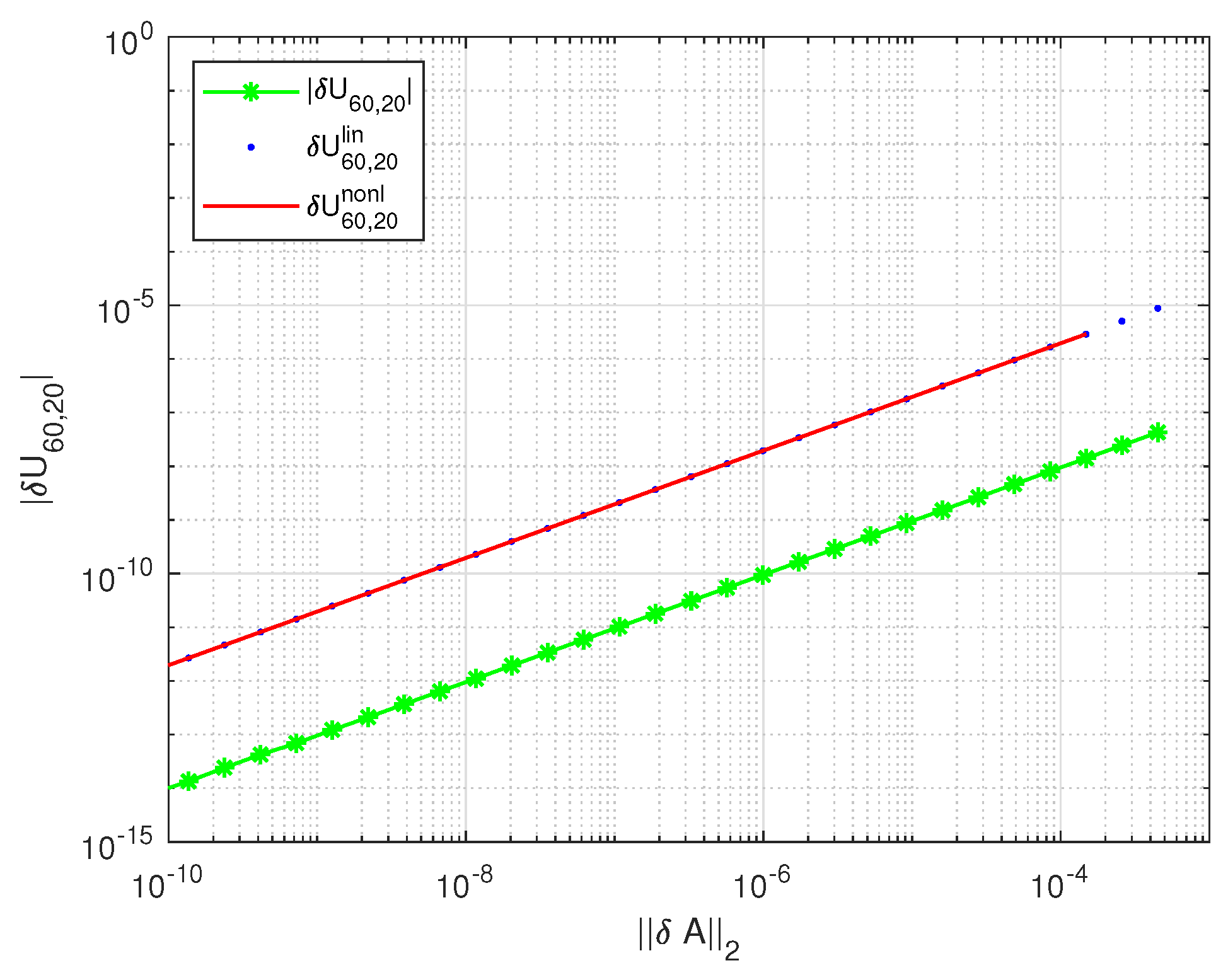
Consider a $100\times 80$ matrix, taken as

$$A=U_0\left[\begin{array}{c}{\Sigma }_0\\ 0\end{array}\right]V_0^T,$$

where ${\Sigma }_0=\mathrm{diag}(1,1,\dots ,1)$, the matrices $U_0$ and $V_0$ are constructed as proposed in [34],

$$\begin{array}{ccc}\hfill U_0& =& M_2{S}_U{M}_1,\hfill \\ \hfill M_1& =& I_m-2e{e}^T/m,M_2=I_m-2f{f}^T/m,\hfill \\ \hfill e& =& {[1,1,1,\dots ,1]}^T,f={[1,-1,1,\dots ,{(-1)}^{m-1}]}^T,\hfill \\ \hfill S_U& =& \mathrm{diag}(1,\sigma ,{\sigma }^2,\dots ,{\sigma }^{m-1}),\hfill \\ & & \\ \hfill V_0& =& N_2{S}_V{N}_1,\hfill \\ \hfill N_1& =& I_n-2g{g}^T/n,N_2=I_n-2h{h}^T/n,\hfill \\ \hfill g& =& {[1,1,1,\dots ,1]}^T,h={[1,-1,1,\dots ,{(-1)}^{n-1}]}^T,\hfill \\ \hfill S_V& =& \mathrm{diag}(1,\tau ,{\tau }^2,\dots ,{\tau }^{n-1}),\hfill \end{array}$$

and the matrices $M_1,M_2,N_1,N_2$ are Householder reflections. The condition numbers of $U_0$ and $V_0$ with respect to the inversion are controlled by the variables σ and τ and are equal to ${\sigma }^{m-1}$ and ${\tau }^{n-1}$, respectively. In the given case, $\sigma =1.05$, $\tau =1.1$ and $\mathrm{cond}(U_0)=125.2,\mathrm{cond}(V_0)=186.2$. The minimum singular value of the matrix A is ${\sigma }_{min}(A)=0.103068025192609$. The perturbation of A is taken as $\delta A={10}^c\times A_0$, where c is a negative number and $A_0$ is a matrix with random entries generated by the MATLAB^®functionrand.

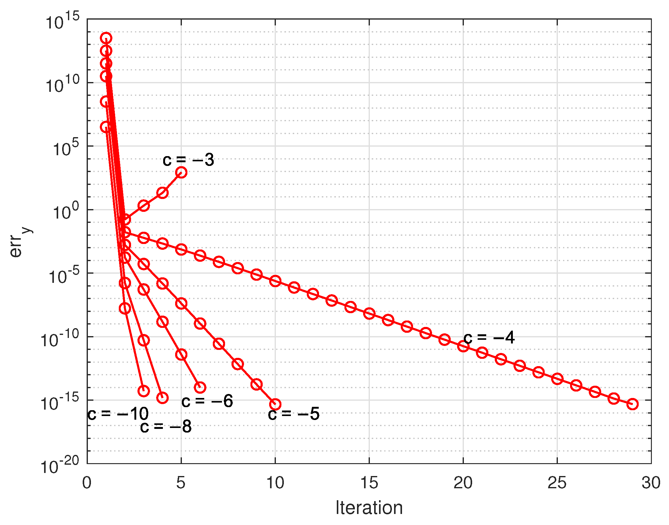
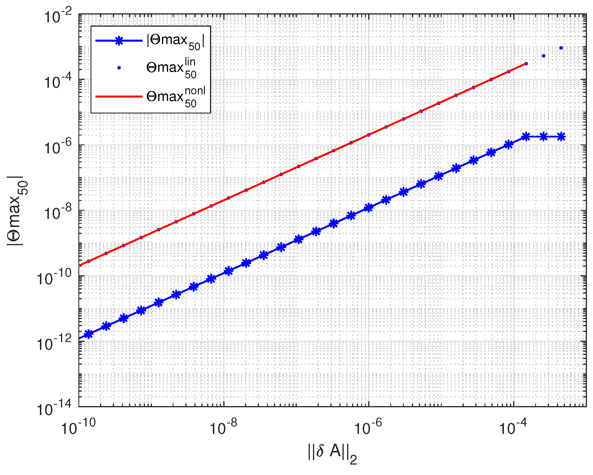
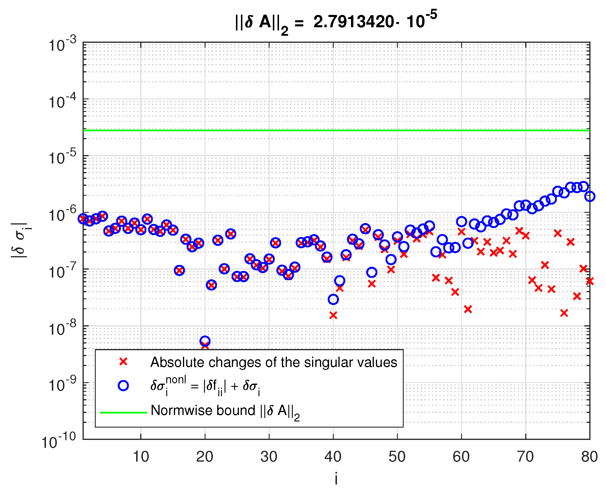
In Figure 10, Figure 11, Figure 12, Figure 13, Figure 14 and Figure 15, we show several results related to the perturbations of the singular value decomposition of A for 30 values of c between $-12$ and $-5$. As particular examples, in Figure 10 we display the perturbations of the entry $U_{60,20}$, which is an element of the matrix $U_1$, and in Figure 11, we display the perturbations of the entry $V_{60,20}$, both as functions of ${\parallel \delta A\parallel }_2$. The componentwise linear bounds correctly reflect the behavior of the actual perturbations and are valid for wide changes in the perturbation size. Note that this holds for all elements of U and V. The global (nonlinear) bounds practically coincide with the linear bounds but do not exist for perturbations whose size is larger than $1.5\times {10}^{-4}$.

Figure 10. Exact values of $|\delta U_{60,20}|$ and the corresponding linear and nonlinear estimates as functions of the perturbation norm.

Figure 11. Exact values of $|\delta V_{60,20}|$ and the corresponding linear and nonlinear estimates as functions of the perturbation norm.

Figure 12. Exact values of $\Phi {\max }_{50}$ and the corresponding linear and nonlinear estimates as functions of the perturbation norm.

Figure 13. Exact values of $\Theta {\max }_{50}$ and the corresponding linear and nonlinear estimates as functions of the perturbation norm.

Figure 14. Perturbations of the singular values and their nonlinear bounds for $\delta A=4.1517085\times {10}^{-10}$.

Figure 15. Perturbations of the singular values and their nonlinear bounds for $\delta A=2.7913420\times {10}^{-5}$.

In Figure 12 and Figure 13, we show the angles between the perturbed and unperturbed left

$${\mathcal{U}}_{50}=\mathrm{span}(u_1,u_2,\dots ,u_{50})$$

and right

$${\mathcal{V}}_{50}=\mathrm{span}(v_1,v_2,\dots ,v_{50})$$

singular subspaces of dimension 50. Again, the linear bounds on the angles $|\Phi \max ({\mathcal{U}}_{50},{\tilde{\mathcal{U}}}_{50})|$ and $|\Theta \max ({\mathcal{V}}_{50},{\tilde{\mathcal{V}}}_{50})|$ are valid for perturbation magnitudes from ${\parallel \delta A\parallel }_2={10}^{-10}$ to ${\parallel \delta A\parallel }_2={10}^{-4}$ and this also holds for singular subspaces of other dimensions. Note that for sufficiently large ${\parallel \delta A\parallel }_2$, the linear estimate also become non-valid.

In Figure 14 and Figure 15, we show the perturbations of the singular values and their nonlinear bounds for two different perturbations with ${\parallel \delta A\parallel }_2=2.7282784\times {10}^{-10}$ and ${\parallel \delta A\parallel }_2=4.3932430\times {10}^{-4}$. While in the first case, the nonlinear bound $\delta {\sigma }_i^{nonl}$ is close to the actual change $\delta {\sigma }_i$ of the singular values, in the second case, the bound becomes significantly greater than the actual change due to the overestimating of the higher-order term ${\Delta }_1$.

From the results shown in Figure 10, Figure 11, Figure 12 and Figure 13, it follows that for the $100\times 80$ matrix in the example under consideration, the overestimates of the perturbations of U and V are approximately 200 times, while the overestimates of $\Phi \max$ and $\Theta \max$ are approximately 100 and 170 times, respectively. In Figure 16 and Figure 17, we show the ratios $\delta U_{ij}^{lin}/\left|\delta U_{ij}\right|,$$i=1,2,\dots ,m;$$j=1,2,\dots ,n$ and $\delta V_{ij}^{lin}/\left|\delta V_{ij}\right|,i=1,2,\dots ,n;j=1,2,\dots ,n$, respectively, along with the corresponding mean values (averages) $E(\delta U_{ij}^{lin}/|\delta U_{ij}|)$ and $E(\delta V_{ij}^{lin}/|\delta V_{ij}|)$ of the ratio for $\delta A={10}^{-8}\times A_0=4.4679\times {10}^{-7}$. The overestimates are mainly due to overestimating the perturbation parameters $x_{(1)},y$ and $x_{(2)}$ in the Equations (36)–(38). In these equations, each entry $\delta A_{ij}$ is replaced by the quantity ${\parallel \delta A\parallel }_2$, leading to an overestimate approximately proportional to m in case of random perturbations. To illustrate this point, in Figure 18 and Figure 19 we show the entries of the matrices $|\delta U_1|$ and $\left|\delta V\right|$, respectively, along with the corresponding componentwise estimates $\delta U^{lin}$ and $\delta V^{lin}$ for $\delta A={10}^{-8}\times A_0=4.4679\times {10}^{-7}$, where the asymptotic estimates are computed for the exact (non approximated) values of the perturbation parameters $x_k=u_i\delta u_j$ and $y_{\ell }=v_i\delta v_j$, obtained by using the exact $\delta A$. Obviously, the estimates are very close to the exact values, which confirms their good quality. The small differences between the actual quantities and their estimates are caused by taking the absolute values of $U,V$ and $\delta W_U,\delta W_V$ in finding the asymptotic bounds $\delta U^{lin}=\left|U\right|\delta W_U^{lin}$ and $\delta V^{lin}=\left|V\right|\delta W_V^{lin}$. We note that the overestimates are inevitable if we want to obtain guaranteed asymptotic perturbation bounds of the SVD elements, and they can be significantly reduced only if we use probability perturbation bounds [28].

Figure 16. The ratio $\delta U_{ij}^{lin}/\left|U_{ij}\right|$ and its mean value for $\delta A={10}^{-8}\times A_0=4.4679\times {10}^{-7}$.

Figure 17. The ratio $\delta V_{ij}^{lin}/V_{ij}$ and its mean value for $\delta A={10}^{-8}\times A_0=4.4679\times {10}^{-7}$.

Figure 18. Values of $|\delta U_{ij}|$ and the corresponding linear estimates for the exact values of $x_k$.

Figure 19. Values of $|\delta V_{ij}|$ and the corresponding linear estimates for the exact values of $y_{\ell }$.

Example 5.

This example visualizes the componentwise estimates of the orthogonal matrices and the singular values for a $200\times 150$ matrix.

Consider a matrix A with $m=200,n=150$, constructed as in the previous example for $\sigma =1.05$ and $\tau =1.0$. The perturbation of A is taken as $\delta A={10}^{-9}\times A_0$, where $A_0$ is a matrix with random entries.

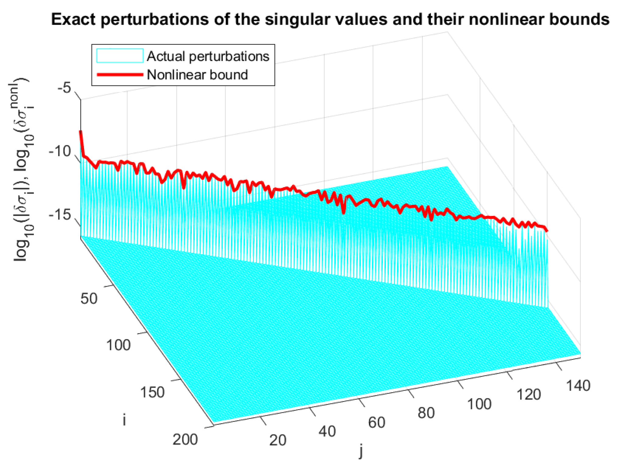
In Figure 20, Figure 21 and Figure 22, we show the entries of the matrix $|\delta U_1|$, the absolute values of the exact changes of all 150 singular values, and the entries of the matrix $\left|\delta V\right|$, respectively, along with the corresponding componentwise estimates $\delta U^{lin}$, $\delta {\sigma }_i^{nonl}$, and $\delta V^{lin}$. The computation of the linear bounds requires the solution of a system of $2q=22350$ linear equations for $x_{(1)}$ and y and $(m-n)m=7500$ equations for $x_{(2)}$. The nonlinear bounds of $\delta U_1$ and $\delta V$ are found only for 7 iterations and are visually indistinguishable from the corresponding linear bounds.

Figure 20. Values of $|\delta U_{ij}|$ and the corresponding linear estimates for a $200\times 150$ matrix.

Figure 21. Perturbations and perturbation bounds of the singular values for a $200\times 150$ matrix.

Figure 22. Values of $|\delta V_{ij}|$ and the corresponding linear estimates for a $200\times 150$ matrix.

The perturbation bounds derived were also tested with higher-order examples, including a $500\times 300$ example.

The examples presented in this section confirm that the new componentwise perturbation bounds of the singular value decomposition can be used efficiently in the analysis of high-order problems and may compare favorably with the known bounds for some particular cases, for instance in the sensitivity analysis of the singular subspaces. The componentwise bounds of the perturbations in the orthogonal matrices U and V in the last example clearly show that for some specific entries the perturbation magnitudes differ ${10}^5$ times and the implementation of normwise perturbation bounds for such examples is not informative. It should also be emphasized that the asymptotic estimates, although not global, ensure valid perturbation bounds for sufficiently large perturbations of the given matrix.

11. Conclusions

The paper presents new results related to the perturbation analysis of the singular value decomposition of a real rectangular matrix of full rank. New asymptotic componentwise perturbation bounds are derived for the orthogonal matrices participating in the decomposition, and an alternative method for computing the sensitivity of the singular subspaces is proposed. The possibility to find non-local bounds is illustrated by using a simple iterative procedure.

A potential disadvantage of the proposed perturbation bounds is their conservatism, i.e., the large difference between the bounds and the corresponding perturbations, especially for large values of m and n. This is due to the necessity to replace the entries of the actual perturbation in the derived bounds by its 2-norm, which leads to pessimistic estimates. This conservatism can be removed using probability perturbation bounds, a matter of further research.

The singular value decomposition perturbation analysis presented in this paper has some peculiarities, making it a challenging problem. On the one hand, the SVD analysis is simpler than other problems, like the perturbation analysis of the orthogonal decomposition to triangular form (the QR decomposition). This is due to the diagonal form of the decomposed matrix, which, among the others, allows the equations for the perturbation parameters to be solved easily, avoiding using the Kronecker product. On the other hand, the presence of two matrices in the decomposition requires the introduction of two different parameter vectors, which are mutually dependent due to the relationship between the perturbations of the two orthogonal matrices. This makes it necessary to solve a coupled system of equations about the parameter vectors, complicating the analysis.

The analysis performed in the paper reveals two reasons for the ill-conditioning of the singular subspaces of a matrix. The first cause is the closeness of some singular values of A, which leads to large elements of the vector $|x_{(1)}|$ and consequently to large entries of the perturbation $|\delta U_1|$. The second reason is the presence of small singular values of A, which is reflected by large elements of the vector $|x_{(2)}|$ and also leads to large values of the respective entries of $|\delta U_1|$. Significantly, these two reasons are independent of each other.