Attacking Robot Vision Models Efficiently Based on Improved Fast Gradient Sign Method

Abstract

The robot vision model is the basis for the robot to perceive and understand the environment and make correct decisions. However, the security and stability of robot vision models are seriously threatened by adversarial examples. In this study, we propose an adversarial attack algorithm, RMS-FGSM, for robot vision models based on root-mean-square propagation (RMSProp). RMS-FGSM uses an exponentially weighted moving average (EWMA) to reduce the weight of the historical cumulative squared gradient. Additionally, it can suppress the gradient growth based on an adaptive learning rate. By integrating with the RMSProp, RMS-FGSM is more likely to generate optimal adversarial examples, and a high attack success rate can be achieved. Experiments on two datasets (MNIST and CIFAR-100) and several models (LeNet, Alexnet, and Resnet-101) show that the attack success rate of RMS-FGSM is higher than the state-of-the-art methods. Above all, our generated adversarial examples have a smaller perturbation than those generated by existing methods under the same attack success rate.

1. Introduction

Nowadays, the robot vision model is widely used in the field of robot vision, such as image classification [1], target detection [2], speech recognition [3], autonomous vehicles [4], etc. Although the robot vision model has achieved success in the field of robot vision, it may suffer from security and robustness problems when feeding with adversarial examples. Adversarial examples are inputs to robot vision models that have been intentionally designed by adding small, imperceptible perturbations [5]. They will cause robot vision models to achieve erroneous results. Influenced by adversarial examples, autonomous vehicles may experience disruptions in their driving state, which can lead to traffic safety issues. Militarily, when using UAVs to detect unknown areas, the adversarial examples will lead to UAV target-identification errors. Apart from these, adversarial examples have a serious impact on the security of all kinds of intelligent system software based on deep neural networks. Memristive chaotic circuits based on CNNs may also be affected [6]. Therefore, the generation method of adversarial examples (adversarial attack method) has gained much attention from researchers. Based on adversarial examples, we can design adversarial defense methods [7,8,9,10] and develop secure and robust intelligent systems.

Currently, adversarial attack methods can be divided into three categories: (1) the gradient-based methods, (2) the optimization-based methods, and (3) the generative adversarial network (GAN)-based methods. The most typical gradient-based method is called the fast gradient sign method (FGSM), which was proposed by Goodfellow et al. [11] in 2015. It computes adversarial examples by maximizing the loss function of the attacked neural network model with the gradient ascent optimizer. Since it can generate adversarial examples efficiently, much research effort has been paid, and many variants have been proposed, including the basic iterative method (BIM, also known as I-FGSM) [12], momentum iterative fast gradient sign method (MI-FGSM) [13], etc. The optimization-based methods [14] directly optimize the distance between the real samples and adversarial examples subject to the misclassification of adversarial examples. The problem with this method is that the added perturbation cannot be constrained properly and may result in invalid adversarial examples [13]. The GAN-based methods [15,16] generate adversarial examples based on generative adversarial networks. These methods train (i) a feed-forward generator network that generates perturbations to create diverse adversarial examples and (ii) a discriminator network to ensure that the generated examples are realistic; once the generator network is trained, it can generate perturbations efficiently for any instance, so as to potentially accelerate adversarial training as defenses. Experiments show that the adversarial examples constructed via the generative adversarial networks have a high attack success rate in the case of defense. However, these kinds of methods are resource-intensive and time-consuming.

In this study, we focus on the gradient-based methods. Compared with other methods, the gradient-based methods are resource-saving and time-efficient. However, since the principle behind the gradient-based methods is the gradient ascent algorithm, just like the gradient descent algorithm, a large learning rate will cause the gradient of the objective function to grow too fast and miss the global optimal solution. A low value will lead to extra iterations and low efficiency. The improper learning rate will cause the problems of large perturbation and low attack success rate. To address this problem, Geoffrey Hinton [17] introduced an adaptive learning rate calculation method, root-mean-square propagation (RMSProp). This method performs a learning rate correction strategy and the exponentially weighted moving average (EWMA) during the gradient update, which can mitigate the problem of rapid gradient growth and keep it efficient. Inspired by the RMSProp algorithm, we efficiently propose an improved RMSProp-based fast gradient sign method, RMS-FGSM, to attack robot vision models. RMS-FGSM generates adversarial examples in an iterative manner. At each iteration, an adaptive learning rate is used to update adversarial examples. Our learning rate is computed based on the EWMA algorithm, which smoothes the change of gradients by considering historical data. Since our method can mitigate the problem of the gradient’s steep growth, adversarial examples can be updated along a stable optimization direction, and the optimal value is highly likely to be achieved; that is, adversarial examples with imperceptible perturbations and a high attack success rate.

The experiments in this study are carried out with several common classification models in robot vision and the environment of Python 3.9, torch 1.13.1, and TorchVision 0.14.1. Two commonly used datasets, MNIST [18] and CIFAR-100 [19], were used. To validate the method, we attacked LeNet [20], Alexnet [1], and Resnet-101 [21]. Experimental results persuasively verify that RMS-FGSM has better performance than other advanced attack methods. Above all, the perturbation of the adversarial examples generated using RMS-FGSM is smaller than other methods under the same attack success rate.

The rest of this study is arranged as follows. Section 2 introduces related work, including the FGSM, BIM, MI-FGSM, and NI-FGSM algorithms. The attack algorithm RMS-FGSM is described in Section 3. In Section 4, we present and analyze the experimental results. And the last section concludes the study.

2. Related Work

In recent years, many gradient-based attack algorithms have been proposed. The process of adversarial attacks can generally be defined as follows: let M be a pre-trained neural network, which can output predicted label y for an input sample x, that is, M(x) = y. J(x, W, y) denotes the loss function of M, where W is the set of weights of model M. Since model M is pre-trained (W is available), we can rewrite J(x, W, y) as J(x, y). The goal of adversarial attacks is to seek an example $x^{*}=x+\eta$ such that $M\left(x^{*}\right)\ne M\left(x\right)$. The noise $\eta$ added to x* should be imperceptible. To this end, the L_p norm of $\eta$ is required to be less than an allowed value $ϵ$ as ${‖x^{*}-x‖}_p\le ϵ$, where p could be 0, 1, 2, and $\infty$.

2.1. Fast Gradient Sign Method

The fast gradient sign method (FGSM) is a one-step gradient-based approach that finds an adversarial example x* by maximizing the loss function J(x, y), which can be formalized as:

$$\underset{x}{\arg \max }(J(x,y))$$

(1)

In order to solve the above problem, the FGSM uses the gradient ascent algorithm, which computes the adversarial noise $\eta$ based on Equation (2):

$$\eta =\epsilon \cdot \mathrm{sign}({\nabla }_{\mathrm{x}}\mathrm{J}(\mathrm{x},\mathrm{y}))$$

(2)

where ∇_x denotes the gradient of loss function J w.r.t. x, $sign\left(·\right)$ is the sign function, and ε is the perturbation factor. The FGSM employs the $L_{\infty }$ norm to validate generated adversarial examples; that is, ${‖\eta ‖}_{\infty }\le ϵ$ should be satisfied.

The FGSM algorithm modifies the image only once based on the gradient calculation, which is time-efficient. However, due to the manually set improper learning rate, in case of the same attack success rate, the perturbation added to the adversarial examples generated using this method will be larger than those of other methods, which will violate the imperceptible requirement.

2.2. Basic Iterative Method

In 2016, Kurakin proposed a FGSM-based basic iterative method (BIM, also known as I-FGSM) to rapidly generate adversarial examples. Different from the one-step attack of the FGSM, the BIM iteratively applies the fast gradient multiple times with a small step size $\alpha$ as shown in Equation (3):

$$x_{t+1}^{*}=Clip\{x_t^{*}+\alpha \cdot sign({\nabla }_{x}J(\theta ,x_t^{*},y))\}$$

(3)

where $x_t^{*}$ denotes the adversarial example obtained at the t-th iteration. In order to make the generated adversarial examples satisfy the $L_{\infty }$ bound, the BIM uses the $Clip\left\{·\right\}$ function to clip $x_t^{*}$ into the $ϵ$ vicinity of x.

Intuitively, the BIM is as easy to understand as the FGSM, concise, and efficient, and the attack effect is obviously better than the FGSM. The author asserted that this approach ensures an optimal pace for gradient ascent, and it is, at worst, equivalent to the FGSM. However, further research has indicated that the samples generated using the BIM lack transferability, resulting in a weak black box attack [22,23,24] effect.

2.3. Momentum Iterative Fast Gradient Sign Method

Dong et al. [25] incorporated the momentum term into the BIM and proposed the MI-FGSM algorithm. As shown in Equation (4), it computes the cumulative gradient g_t+1 by a weighted sum of gradients obtained in the past t-th iterations, where µ is a decay factor. Based on the cumulative gradient, it computes the adversarial example $x_{t+1}^{*}$ by adding a small perturbation to $x_t^{*}$, as shown in Equation (5), where α is a step size. At each iteration, the current gradient ${\nabla }_{x}J(x_t^{*},y)$ is normalized by the L₁ distance of itself.

$$g_{t+1}=\mu g_t+\frac{{\nabla }_{x}J(x_t^{*},y)}{\left|\right|{\nabla }_{x}J(x_t^{*},y)|{|}_1}$$

(4)

$$x_{t+1}^{*}=x_t^{*}+\alpha \ast sign(g_{t+1})$$

(5)

According to the principle of momentum in physics, the iterative calculation process of adversarial examples can be accelerated. In addition, with the help of momentum, the optimization process can go beyond local maxima and is more likely to reach a global maximum. Since the update direction becomes more stable, the MI-FGSM is more efficient and has better transferability [26,27] across different neural networks. However, this method may increase the gradient too rapidly and introduce a large perturbation to adversarial examples.

2.4. Nesterov Iterative Fast Gradient Sign Method

Lin et al. [28] leveraged the Nesterov accelerated gradient (NAG) [29] and presented the NI-FGSM algorithm so that it can improve transferability. The NI-FGSM makes a jump in the direction of previously accumulated gradients before computing the gradients in each iteration. It substitutes $x_t^{*}$ in Equation (4) with $x_t^{adv}+\alpha ·\mu ·g_t$ to leverage the looking-ahead property of the NAG and build a robust adversarial attack. Such looking ahead property of the NAG can help to escape from poor local maxima easier and faster, resulting in the improvement in transferability.

3. Our Technique

3.1. Method Framework

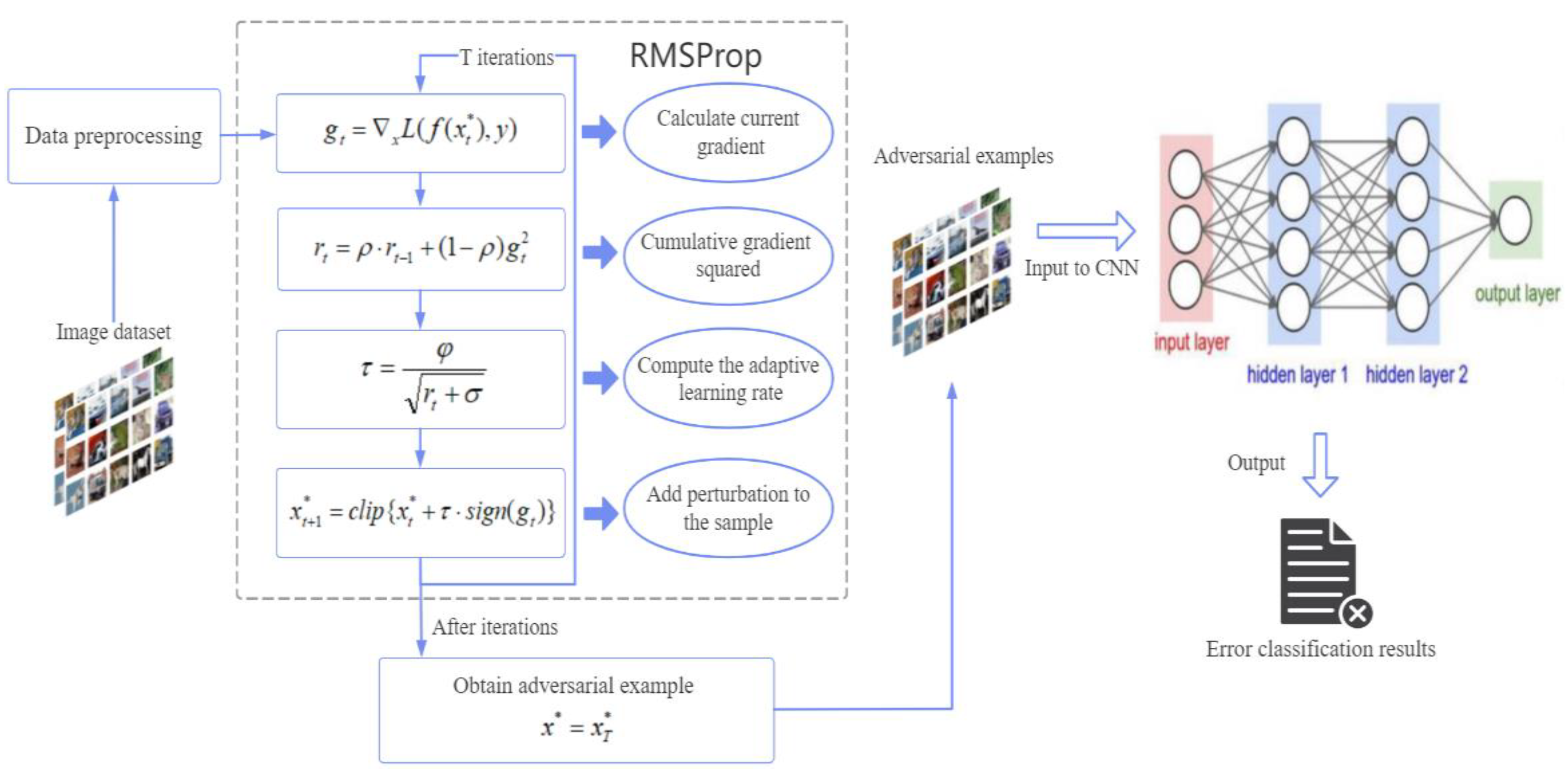
The process of the RMS-FGSM adversarial attack is shown in Figure 1; once the image dataset is input, preprocess the data and calculate the current gradient g_t of the loss function. Next, compute the exponential average r_t of the squared gradients with EWMA to prepare for the next step, and the parameter ρ is used as a weight parameter to control the acquisition of a historical cumulative squared gradient and a new squared gradient. Then, the learning rate $\tau$ is calculated, where the exponential average r_t from the previous step controls the size of the learning rate. When g_t increases, the learning rate decreases; conversely, when g_t decreases, the learning rate increases to achieve the adaptive learning rate. Then, calculate the current perturbation value using the sign function and add it to the original example to generate a new adversarial example and proceed to the next iteration. After the number of iterations reaches a fixed value T, we can obtain the optimal adversarial example, and the perturbation of the adversarial example is imperceptible for humans. Finally, the adversarial example is input into the attacked neural network model, which will lead to the wrong classification results.

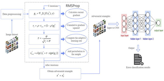
Figure 1. The overall framework of our method.

3.2. Fast Gradient Sign Method Based on Adaptive Learning Rate

The fast gradient sign method (FGSM) is able to generate adversarial examples efficiently based on the gradient ascend approach. However, as shown in Equation (2), a fixed learning rate ε is used to compute the perturbation, which may lead to slow convergence or even failure to converge. Additionally, a fixed learning rate may fail to adapt to different samples, which may result in insufficient updates for some samples to reach optimal solutions. Above all, the missing of the optimal solution may introduce a large perturbation to adversarial examples and decrease the attack success rate. Although some improved variant methods such as I_FGSM and MI_FGSM have been proposed, they also employ a fixed step size $\alpha$ as shown in Equations (3) and (5). In order to further improve the performance of the gradient-based adversarial attack methods, we propose the RMS-FGSM, which utilizes the adaptive learning rate calculation method RMSProp.

Let $f\left(x;W,b\right)=y$ be a neural network model, such as the Alexnet for image classification tasks. W and b are the weight matrix and offset vector, respectively. When feeding with an image sample x, the model will output prediction result y. In the training process of neural networks, we always construct a loss function of the network $L\left(f\right(x;W,b),y)$ and reduce the training of neural networks to an optimization problem as follows:

$$\underset{W,b}{\arg \min }(L(f(x;W,b),y))$$

(6)

In order to resolve the optimization problem, a frequently used approach is the gradient descent, which calculates the optimal W and b along the direction of the gradients ${\nabla }_{W}L\left(f\right(x;W,b),y)$ and ${\nabla }_{b}L\left(f\right(x;W,b),y)$, respectively. During this process, a labeled training dataset $D=\left\{(x,y) | x is an input image sample, y is the corresponding classification label\right\}$ will be used.

Different from the above training process, the white-box adversarial attack methods assume that the neural network model $f\left(x;W,b\right)$ is pre-trained. Therefore, the weight matrix W and offset vector b are both available. The purpose of the adversarial attack is to generate difference-inducing input samples. Formally, given an image sample x with a label y, an adversarial attack aims to generate an adversarial example x* by adding an imperceptible perturbation to x, such that $f(x;W,b)\ne y$. This problem can be addressed by maximizing the loss between label y and the prediction $f(x;W,b)$. Formally, we have the following optimization problem (we neglect W and b because they are available):

$$\underset{x}{\arg \max }(L(f(x),y))$$

(7)

In this study, we address the problem with the gradient ascent algorithm. Different from the FGSM and its variants, the RMS-FGSM calculates the adversarial examples based on an adaptive learning rate given by RMSProp. RMSProp is a variant of the gradient descent algorithm used to adjust model parameters. The most distinctive feature of RMSProp is that it can adaptively adjust the learning rate of different parameters by combining the first-order and second-order moments. By utilizing the smooth nature of the square root function, it can avoid the problems of drastic changes and unstable behavior in the parameter space. The RMS-FGSM computes adversarial examples in an iterative manner as follows:

$$g_t={\nabla }_{x}L(f(x_t^{*}),y)$$

(8)

$$r_t=\rho \cdot r_{t-1}+(1-\rho )g_t^2$$

(9)

$$\tau =\frac{\varphi }{\sqrt{r_t+\sigma }}$$

(10)

$$x_{t+1}^{*}=clip\{x_t^{*}+\tau \cdot sign(g_t)\}$$

(11)

where g_t is the gradient of loss function $L\left(f\right(x_t^{*}),y)$ w.r.t x at the t-th iteration. $x_t^{*}$ denotes the adversarial example achieved at the t-th iteration. Specifically, $x_0^{*}=x$, f(x) = y. In order to adjust the learning rate of adversarial examples, the RMS-FGSM computes an exponential average r_t of the squared gradients based on the EWMA at each iteration according to Equation (9). This is essentially an exponentially decreasing weighted moving average, where the weight of each squared gradient decreases exponentially over time. The square of g_t aims to eliminate the effect of the gradient sign. ρ is a constant that is typically set to 0.9. It determines the speed of weight decay of historical gradients, with smaller values resulting in faster decay. The aim of the decay factor ρ is to decrease the influence of historical gradients on the computation of the exponential average. Based on the exponential average, the RMS-FGSM calculates the learning rate $\tau$ according to Equation (10), where $\phi$ represents the initial learning rate, and $\sigma$ is usually set to 10⁻⁶ to prevent the denominator from being zero. As we can see, if the gradient is large, the learning rate will be suppressed; if the gradient is small, the learning rate will be increased. Different from the usual use case of RMSProp, the essence of our adversarial attack method is the gradient ascent rather than the gradient descent algorithm. Consequently, the RMS-FGSM updates the adversarial examples by adding (rather than subtracting) the computed perturbation $\tau \cdot sign\left(g_t\right)$ according to Equation (11). Additionally, in order to achieve imperceptible adversarial examples, we use the $clip\left\{·\right\}$ function to impose the bounding constraint ${‖x^{*}-x‖}_2\le ϵ$. The algorithm stops when the specified number of iterations is reached; then, we obtain the adversarial examples.

In conclusion, our approach has the following advantages: (1) Different adversarial examples have different learning rates, and the learning rate varies according to gradients during the iterative calculation process. This is completely different from the previous FGSM and variant algorithms with a fixed learning rate. (2) The problems of drastic changes and unstable behavior incurred by the fixed learning rate can be mitigated. (3) Based on the adaptive learning rate, it is more likely to achieve optimal adversarial examples while keeping a high convergence speed. (4) Our adversarial examples may have a small perturbation. (5) Since optimal adversarial examples with a small perturbation can be obtained, our approach may have a high attack success rate. (6) The high convergence speed makes our method time-efficient.

3.3. RMS-FGSM Algorithm

The process of generating adversarial samples using the RMS-FGSM algorithm is as follows: 1. Given an original image x; 2. Input x to classifier f(x) and calculate its gradient g_t of loss function w.r.t x.; 3. According to g_t, compute an exponential average r_t of the squared gradients based on the EWMA; 4. Calculate the adaptive learning rate $\tau$ according to r_t; 5. Calculate the perturbation pixel by pixel, add it to x, and use the $clip\left\{·\right\}$ function to prevent pixels from going out of range; 6. Repeat steps 2 to 5 until the specified number of iterations is reached.

The outline of our the RMS-FGSM algorithm framework is shown in Algorithm 1.

Algorithm 1: RMS-FGSM.

Input: A classifier f with loss function L; original image x; ground-truth label y; decay rate ρ; number of iterations T; initial learning rate $\phi$; Output: Adversarial example x*; 1: Initialize the variable r0 = 0; $x_0^{*}=x$; 2: For t = 0 to T-1 do: 3: Input $x_t^{*}$ to classifier f; 4: Calculate the current gradient: $g_t={\nabla }_{x}L(f(x_t^{*}),y)$; 5: Cumulative squared gradient: $r_t=\rho \cdot r_{t-1}+(1-\rho )g_t^2$; 6: Compute the adaptive learning rate: $\tau =\frac{\varphi }{\sqrt{r_t+\sigma }}$; 7: Add perturbation to the sample: $x_{t+1}^{*}=clip\{x_t^{*}+\tau \cdot sign(g_t)\}$; 8: End for 9: return $x^{*}=x_T^{*}$.

4. Experiments

4.1. Experimental Setup

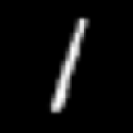
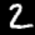
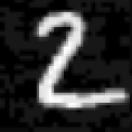
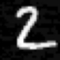
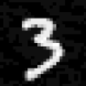
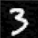
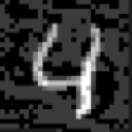
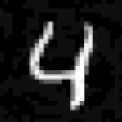
Datasets. We evaluate our method based on two commonly used datasets, MNIST and CIFAR-100. The MNIST dataset is a subset of the NIST (National Institute of Standards and Technology) dataset. It has a total of 70,000 images, including 60,000 in the training set and 10,000 in the test set. Each image is a 28 × 28 pixel image of 0–9 gray scale handwritten digits with white text on a black background. The CIFAR-100 dataset is a small dataset for recognizing pervasive objects. Consisting of 60,000 32 × 32 pixel images, it has 100 classes, and each class contains 600 images with 500 training images and 100 test images. The 100 classes in CIFAR-100 are divided into 20 superclasses. Each image has a “fine” label (the class it belongs to) and a “coarse” label (the superclass it belongs to).

Implementation details. A set of different epsilon values (EPS) represents the initial learning rate in the BIM, MI-FGSM, NI-FGSM, and RMS-FGSM, and it is actually the perturbation factor in the FGSM method. Our experimental results are based on the L₂ norm and non-target attack. The decay factor ρ in our RMS-FGSM is set to 0.9, and the number of iterations T in the BIM, MI-FGSM, NI-FGSM, and RMS-FGSM is set to 10. Our experiments run on a machine with an Intel Core i7-8700K CPU, 32 GB memory, and an Nvidia GeForce GTX 1080Ti graphics card (11 GB memory). We use Python 3.9, Torch 1.13.1, TorchVision 0.14.1, and related libraries.

Evaluation metrics. For the performance evaluation and comparison, we use three different metrics, including the perturbation value (l₂) calculated for different initial learning rates, average attack success rate (Avg asr), and average perturbation value (Avg per).

4.2. Experimental Method

Several common classification models in robot vision are used for our experiments. In order to verify the advantages of the proposed method, we designed two experiments to verify that the proposed method is superior to other methods in terms of effectiveness and imperceptibility. (1) In experiment 1, we set MNIST as the dataset and the LeNet model as the experimental model. Firstly, a set of different epsilon values (0, 0.05, 0.1, 0.15, 0.2, 0.25, 0.3, 0.35, and 0.4) were used as the initial learning rate to generate adversarial examples on the MNIST with the FGSM, BIM, MI-FGSM, NI-FGSM, and RMS-FGSM algorithm, respectively. Then, we analyzed the experimental results to compare the effectiveness and imperceptibility of the adversarial examples generated by these different methods with different initial learning rates. (2) In experiment 2, we set CIFAR-100 as the dataset and Alexnet and Resnet-101 as the experimental models. Generate adversarial examples on both models using the same methods as in experiment 1. And analyze the experimental results to compare the effectiveness and imperceptibility of the adversarial examples generated using these different methods on different models.

4.3. Adversarial Attack Based on MNIST

We first perform a white-box attack on the LeNet network using different methods, including the FGSM, BIM, MI-FGSM, NI-FGSM, and RMS-FGSM algorithms, to demonstrate the effectiveness of our method. Table 1 presents the results of experiment 1 on the MNIST dataset. In addition, we also calculate and plot the prediction accuracy of LeNet with the FGSM and RMS-FGSM methods under different epsilon values in Figure 2, which represents the proportion of test samples that predicted correctly over all test samples.

Table 1. The experimental results of experiment 1 based on MNIST and LeNet ¹.

EPS	Input	La	FGSM			BIM			MI-FGSM			NI-FGSM			RMS-FGSM
			Adv	Ar	l2	Adv	Ar	l2	Adv	Ar	l2	Adv	Ar	l2	Adv	Ar	l2
0		1		1	0		1	0		1	0		1	0		1	0
0.05		2		2	1.374		5	0.876		7	0.884		4	0.816		8	0.745
0.1		3		8	2.753		8	0.982		9	0.975		7	0.828		7	0.776
0.15		4		9	4.081		9	1.078		9	0.978		6	0.854		5	0.792
0.2		5		2	5.517		8	1.146		6	1.042		9	0.873		8	0.804
0.25		6		0	6.878		0	1.177		4	1.078		8	0.883		9	0.801
0.3		7		2	8.149		5	1.216		8	1.106		3	0.907		2	0.806
0.35		8		5	9.591		6	1.223		5	1.149		9	0.915		6	0.813
0.4		9		2	10.969		1	1.275		4	1.178		2	0.902		5	0.809
Avg asr			72.6%			84.5%			86.4%			89.6%			91.6%
Avg per			5.479			0.997			0.932			0.775			0.705

¹ La: the true label of the original image; Adv: the generated adversarial example image; Ar: the prediction label given using the model.

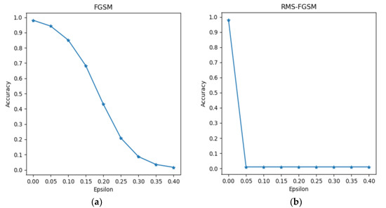
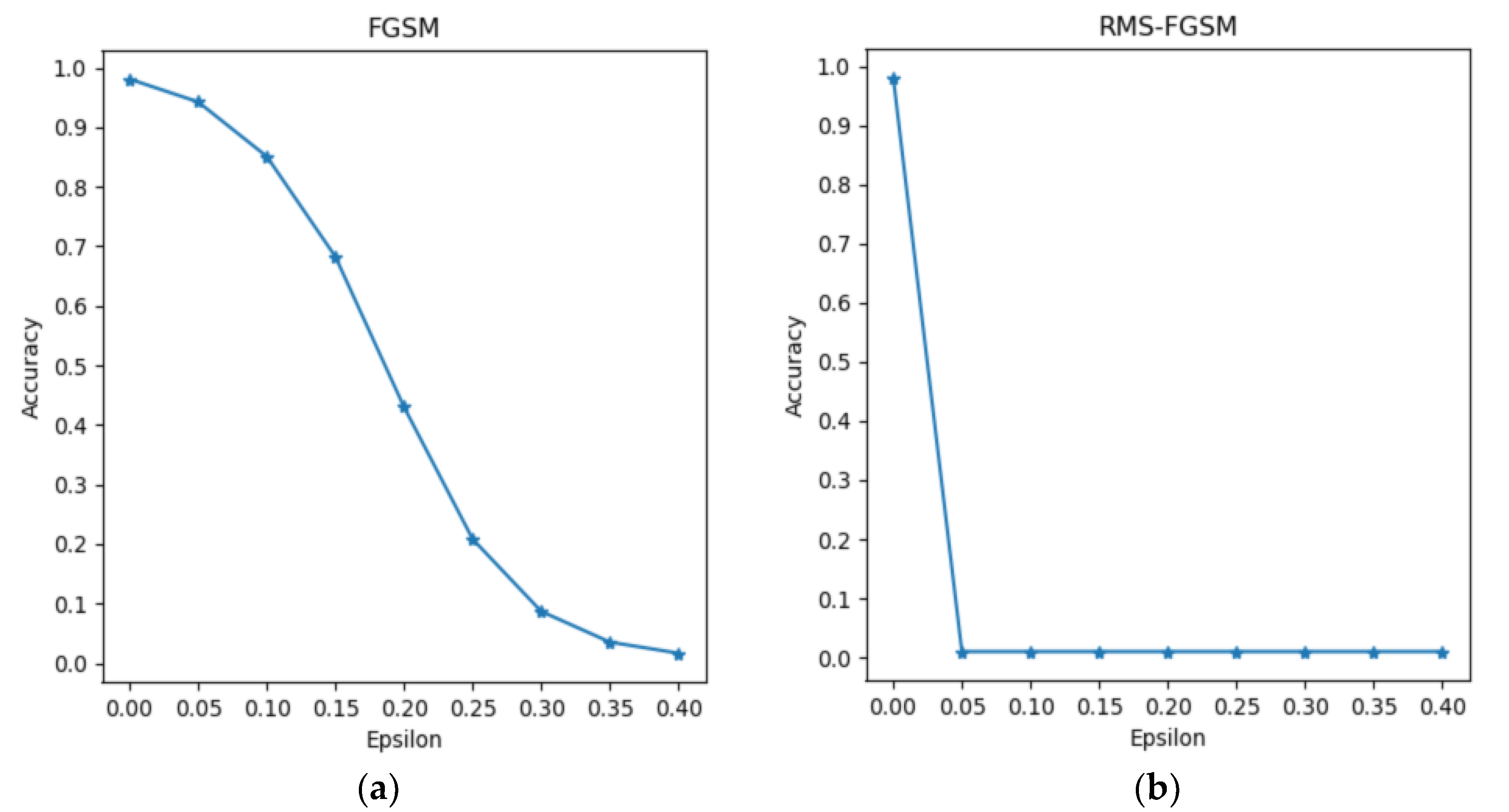
Figure 2. The prediction accuracy in the FGSM (a) and RMS-FGSM (b) methods when attacking the LeNet model. Accuracy represents the proportion of test samples that predicted correctly over all test samples; the lower prediction accuracy of the model indicates the higher attack success rate of the adversarial method. As EPS increases, the accuracy in RMS-FGSM decreases faster than that in FGSM and tends to converge.

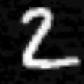
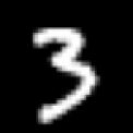
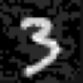
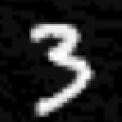
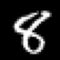
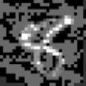
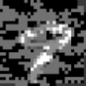
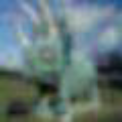
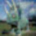
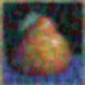
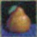
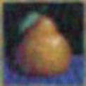
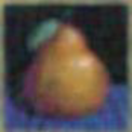
As we can see from Table 1, as the EPS increases, the l₂ of the adversarial examples with the FGSM also increases. The EPS is actually the perturbation factor of Equation (2) in the FGSM. At the same time, the l₂ values in the BIM, MI-FGSM, and NI-FGSM methods are slowly increasing, while the l₂ in the RMS-FGSM has been maintained at around 0.8. From the images, the perturbation of the adversarial examples in the FGSM can be easily recognized by humans, but the perturbations in the BIM, MI-FGSM, NI-FGSM, and RMS-FGSM methods are small. Furthermore, we also calculate the average attack success rate (Avg asr) and average perturbation value (Avg per) in these methods. The results show that the FGSM, BIM, MI-FGSM, and NI-FGSM methods obtain average attack success rates of 72.6%, 84.5%, 86.4%, and 89.6%, respectively, and the average attack success rate of the RMS-FGSM reaches 91.6%, which is the highest of these methods. The average perturbation value of the RMS-FGSM is 0.705, which is also the lowest among the methods.

In Figure 2, we can confirm that the accuracy of the model gradually decreases as the EPS increases in the FGSM method. However, the accuracy of the model in the RMS-FGSM is not affected by the initial learning rate, and finally maintains at about 0.01, which is much lower than the accuracy in the FGSM. This means that the RMS-FGSM is able to find the global optimal solution using the exponentially weighted moving average and adaptive learning rate, and it is not affected by the initial learning rate.

4.4. Adversarial Attack Based on CIFAR-100

In experiment 2, we also perform a white-box attack with the methods in experiment 1, but we use the CIFAR-100 dataset on Alexnet and Resnet-101, respectively. Table 2 and Table 3 show the results of experiment 2 on the CIFAR-100 dataset and two different models.

Table 2. The experimental results of experiment 2 based on CIFAR-100 and Alexnet.

EPS	Input	La	FGSM			BIM			MI-FGSM			NI-FGSM			RMS-FGSM
			Adv	Ar	l2	Adv	Ar	l2	Adv	Ar	l2	Adv	Ar	l2	Adv	Ar	l2
0		11		11	0		11	0		11	0		11	0		11	0
0.05		23		83	1319.89		52	2168.72		43	2749.18		71	2883.94		7	2331.99
0.1		38		58	2631.59		57	2373.98		55	2950.84		66	3004.96		36	2422.59
0.15		42		28	3959.67		94	2584.86		67	2989.19		4	3041.01		46	2425.45
0.2		51		39	5278.10		47	2832.27		13	3055.10		48	3076.21		39	2422.92
0.25		65		48	6439.86		55	3084.59		73	3024.25		52	3103.83		60	2392.04
0.3		74		29	7917.18		74	3113.83		85	3078.15		22	3064.81		65	2413.65
0.35		88		41	9239.20		54	3152.67		93	3126.84		32	3105.91		83	2433.23
0.4		96		3	10,304.54		79	3088.63		66	3093.78		52	3093.25		45	2424.46
Avg asr			72.4%			83.5%			90.2%			92.8%			94.6%
Avg per			5232.22			2488.83			2674.14			2708.21			2140.7

Table 3. The experimental results of experiment 2 based on CIFAR-100 and Resnet-101.

EPS	Input	La	FGSM			BIM			MI-FGSM			NI-FGSM			RMS-FGSM
			Adv	Ar	l2	Adv	Ar	l2	Adv	Ar	l2	Adv	Ar	l2	Adv	Ar	l2
0		15		15	0		15	0		15	0		15	0		15	0
0.05		29		86	1318.59		96	2246.92		7	2860.22		96	2918.59		78	2298.88
0.1		36		45	2629.47		73	2414.55		67	2967.01		67	2967.01		33	2507.00
0.15		45		13	3951.65		76	2599.35		37	3003.38		18	3058.88		61	2417.71
0.2		57		81	5279.56		83	2828.45		29	3052.83		10	3072.11		80	2425.84
0.25		68		48	6598.16		11	3023.82		62	3103.63		59	3103.83		43	2402.16
0.3		75		29	7883.54		5	3089.71		44	3099.17		93	3100.97		35	2422.22
0.35		84		23	9231.48		78	3096.01		80	3103.81		94	3106.59		98	2461.51
0.4		92		76	10,459.62		62	3112.46		64	3109.20		6	3101.57		49	2400.20
Avg asr			81.9%			97.3%			99.1%			99.6%			99.9%
Avg per			5261.48			2499.03			2699.14			2714.39			2148.39

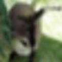
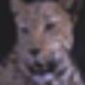
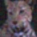
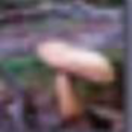
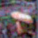
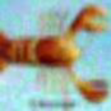
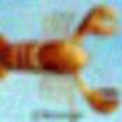
From the experimental results in Table 2, when the EPS is 0.05, the l₂ of the FGSM is 1319.89, which is smaller than those of other methods. However, the l₂ of the FGSM far exceeds those of other methods as the EPS changes, resulting in a large perturbation on the adversarial example images. The l₂ in the BIM, MI-FGSM, and NI-FGSM methods slightly changes as EPS increases but stably remains around 2400 in the RMS-FGSM. In Table 2, we also observe that the RMS-FGSM has the highest average attack success rate of 94.6% on Alexnet, while the FGSM, BIM, MI-FGSM, and NI-FGSM methods obtain an average attack success rate of 72.4%, 83.5%, 90.2%, and 92.8%, respectively. The average perturbation value of the RMS-FGSM is 2140.7 on Alexnet, which has a smaller perturbation on adversarial images.

Then, Table 3 shows the results of experiment 2 on Resnet-101. It can be seen that the l₂ of the FGSM increases rapidly as the EPS changes; there is also a slight increase for the BIM, MI-FGSM, and NI-FGSM methods, while the l₂ of the RMS-FGSM is always maintained at a small value. In addition, the RMS-FGSM reaches a slightly higher average attack success rate of 99.9% on Resnet-101 compared with 99.1% and 99.6% in the MI-FGSM and NI-FGSM. However, our attack method obtains a significantly lower average perturbation value of 2148.39 compared with other methods.

Such experimental results suggest that the RMS-FGSM finds the global optimum point in the process of generating adversarial examples and produces an imperceptible perturbation so that there is only an extremely small difference between the adversarial example and the original example. In addition, with the change in the initial learning rate, the perturbation value generated using the previous methods also fluctuates, while the perturbation value generated using our method remains at a small value. The experimental results on two different models suggest that our RMS-FGSM method is more effective at misleading a white-box network.

5. Conclusions

In this study, we focus on the gradient-based method and improve the fast gradient sign method. The gradient-based method is a kind of efficient and typical attack approach. However, this kind of method is likely to suffer from the problems of large perturbation value and low attack success rate. In this study, we propose an adversarial attack algorithm based on root-mean-square propagation. By integrating with the RMSProp, RMS-FGSM is more likely to generate optimal adversarial examples, and a high attack success rate can be achieved. The experimental results convincingly verified that the performance of the RMS-FGSM is better than the other methods when generating adversarial examples on the MNIST and CIFAR-100 datasets. Furthermore, the adversarial examples generated using the RMS-FGSM have a smaller perturbation under the same attack success rate.

References

- Krizhevsky, A.; Sutskever, I.; Hinton, G.E. Imagenet classification with deep convolutional neural networks. In Proceedings of the 26th Annual Conference on Neural Information Processing Systems, Lake Tahoe, NV, USA, 3–6 December 2012. [Google Scholar]
- Xie, C.; Wang, J.; Zhang, Z.; Zhou, Y.; Xie, L.; Yuille, A. Adversarial Examples for Semantic Segmentation and Object Detection. In Proceedings of the IEEE International Conference on Computer Vision, Venice, Italy, 22–29 October 2017. [Google Scholar]
- Cisse, M.; Adi, Y.; Neverova, N.; Keshet, J. Houdini: Fooling deep structured prediction models. arXiv 2017, arXiv:1707.05373. [Google Scholar]
- Bojarski, M.; Del Testa, D.; Dworakowski, D.; Firner, B.; Flepp, B.; Goyal, P.; Jackel, L.D.; Monfort, M.; Muller, U.; Zhang, J.; et al. End to end learning for self-driving cars. arXiv 2016, arXiv:1604.07316. [Google Scholar]
- Szegedy, C.; Zaremba, W.; Sutskever, I.; Bruna, J.; Erhan, D.; Goodfellow, I.; Fergus, R. Intriguing properties of neural networks. In Proceedings of the 2nd International Conference on Learning Representations, Banff, AB, Canada, 14–16 April 2014. [Google Scholar]
- Buscarino, A.; Fortuna, L.; Frasca, M.; Gambuzza, L.V.; Sciuto, G. Memristive chaotic circuits based on cellular nonlinear networks. Int. J. Bifurc. Chaos 2012, 22, 1250070. [Google Scholar] [CrossRef]
- Zhang, H.; Yu, Y.; Jiao, J.; Xing, E.; El Ghaoui, L.; Jordan, M. Theoretically principled trade-off between robustness and accuracy. In Proceedings of the International Conference on Machine Learning (ICML), Long Beach, CA, USA, 9–15 June 2019; pp. 7472–7482. [Google Scholar]
- Wong, E.; Kolter, Z. Provable defenses against adversarial examples via the convex outer adversarial polytope. In Proceedings of the International Conference on Machine Learning (ICML), San Diego, CA, USA, 3–5 May 2018; pp. 5286–5295. [Google Scholar]
- Tram’er, F.; Kurakin, A.; Papernot, N.; Goodfellow, I.J.; Boneh, D.; McDaniel, P.D. Ensemble adversarial training: Attacks and defenses. In Proceedings of the International Conference on Learning Representations (ICLR), Vancouver, BC, Canada, 30 April–3 May 2018. [Google Scholar]
- Madry, A.; Makelov, A.; Schmidt, L.; Tsipras, D.; Vladu, A. Towards deep learning models resistant to adversarial attacks. In Proceedings of the International Conference on Learning Representations (ICLR), Vancouver, BC, Canada, 30 April–3 May 2018. [Google Scholar]
- Goodfellow, I.J.; Shlens, J.; Szegedy, C. Explaining and harnessing adversarial examples. In Proceedings of the International Conference on Learning Representations, San Diego, CA, USA, 7–9 May 2015. [Google Scholar]
- Kurakin, A.; Goodfellow, I.; Bengio, S. Adversarial examples in the physical world. In Proceedings of the International Conference on Learning Representations Workshop, Toulon, France, 24–26 April 2017. [Google Scholar]
- Dong, Y.; Liao, F.; Pang, T.; Su, H.; Hu, X.; Li, J.; Zhu, J. Boosting adversarial attacks with momentum. arXiv 2017, arXiv:1710.06081. [Google Scholar]
- Carlini, N.; Wagner, D. Towards Evaluating the Robustness of Neural Networks. In Proceedings of the IEEE Symposium on Security and Privacy (SP), San Jose, CA, USA, 22–26 May 2017. [Google Scholar]
- Xie, P.; Shi, S.; Xie, W.; Qin, R.; Hai, J.; Wang, L.; Chen, J.; Hu, G.; Yan, B. Improving the Transferability of Adversarial Examples by Using Generative Adversarial Networks and Data Enhancement. J. Phys. Conf. Ser. 2022, 2203, 012026. [Google Scholar] [CrossRef]
- Hu, S.; Liu, X.; Zhang, Y.; Li, M.; Zhang, L.Y.; Jin, H.; Wu, L. Protecting Facial Privacy: Generating Adversarial Identity Masks via Style-robust Makeup Transfer. arXiv 2022, arXiv:2203.03121. [Google Scholar]
- Tieleman, T.; Hinton, G. Lecture 6.5-rmsprop: Divide the gradient by a running average of its recent magnitude. Coursera Neural Netw. Mach. Learn. 2012, 4, 26–31. [Google Scholar]
- The Mnist Database of Handwritten Digits. Available online: http://yann.lecun.com/exdb/mnist/ (accessed on 11 June 2023).
- The CIFAR-10 Dataset. Available online: http://www.cs.toronto.edu/~kriz/cifar.html (accessed on 2 July 2023).
- Lecun, Y.; Bottou, L. Gradient-based learning applied to document recognition. Proc. IEEE 1998, 86, 2278–2324. [Google Scholar] [CrossRef]
- He, K.; Zhang, X.; Ren, S.; Sun, J. Deep residual learning for image recognition. In Proceedings of the IEEE Conference on Computer Vision and Pattern Recognition, Las Vegas, NV, USA, 27–30 June 2016; pp. 770–778. [Google Scholar]
- Akhtar, N.; Mian, A. Threat of adversarial attacks on deep learning in computer vision: A survey. IEEE Access 2018, 6, 14410–14430. [Google Scholar] [CrossRef]
- Wu, T.; Luo, T.; Ii, D.C.W. Black-Box Attack using Adversarial Examples: A New Method of Improving Transferability. World Sci. Annu. Rev. Artif. Intell. 2023, 1, 2250005. [Google Scholar] [CrossRef]
- Ji, Y.; Zhou, G. Improving Adversarial Attacks with Ensemble-Based Approaches. In Proceedings of the CAAI International Conference on Artificial Intelligence, Beijing, China, 27–28 August 2022; Springer: Cham, Switzerland, 2022. [Google Scholar]
- G’eron, A. Hands-on Machine Learning with Scikit-Learn and Tensorflow: Concepts, Tools, and Techniques to Build Intelligent Systems; O’Reilly Media, Inc.: Sebastopol, CA, USA, 2017. [Google Scholar]
- Papernot, N.; McDaniel, P.; Goodfellow, I. Transferability in machine learning: From phenomena to black-box attacks using adversarial samples. arXiv 2016, arXiv:1605.07277. [Google Scholar]
- Naseer, M.; Khan, S.H.; Rahman, S.; Porikli, F. Distorting neural representations to generate highly transferable adversarial examples. arXiv 2018, arXiv:1811.09020. [Google Scholar]
- Lin, J.; Song, C.; He, K.; Wang, L.; Hopcroft, J.E. Nesterov accelerated gradient and scale invariance for adversarial attacks. In Proceedings of the International Conference on Learning Representations, Addis Ababa, Ethiopia, 26–30 April 2020. [Google Scholar]
- Nesterov, Y. A method for unconstrained convex minimization problem with the rate of convergence o(1/k2). Dokl. Akad. Nauk. USSR 1983, 269, 543–547. [Google Scholar]
Disclaimer/Publisher’s Note: The statements, opinions and data contained in all publications are solely those of the individual author(s) and contributor(s) and not of MDPI and/or the editor(s). MDPI and/or the editor(s) disclaim responsibility for any injury to people or property resulting from any ideas, methods, instructions or products referred to in the content. |
© 2024 by the authors. Licensee MDPI, Basel, Switzerland. This article is an open access article distributed under the terms and conditions of the Creative Commons Attribution (CC BY) license (https://creativecommons.org/licenses/by/4.0/).