Abstract
The utilization of the Monte Carlo method in conjunction with probabilistic seismic hazard analysis (PSHA) constitutes a compelling avenue for exploration. This approach presents itself as an efficient and adaptable alternative to conventional PSHA, particularly when confronted with intricate factors such as parameter uncertainties and diverse earthquake source models. Leveraging the Monte Carlo method and drawing from the widely adopted Cornell-type seismicity model in engineering seismology and disaster mitigation, as well as a seismicity model capturing temporal, spatial, and magnitude inhomogeneity, we have derived a formula for the probability of earthquake intensity occurrence and the mean rate of intensity occurrence over a specified time period. This effort has culminated in the development of a MATLAB-based program named MCPSHA. To assess the model’s efficacy, we selected Baoji City, Shaanxi Province, China, as our research site. Our investigation delves into the disparity between occurrence probability and extreme probability (a surrogate commonly employed for occurrence probability) in the Baoji region over the next 50 years. The findings reveal that the Western region of Baoji exhibits a heightened hazard level, as depicted in the maps, which illustrate a 10% probability of exceedance within a 50-year timeframe. The probability of earthquake occurrence under various intensities (VI, VII, and VIII) over 50 years follows a declining trend from west to east. Furthermore, the likelihood of seismic intensity exceeding VI, VII, and VIII indicates the lowest exceeding probability in the northeast and the highest in the northwest. Notably, for intensities VI-VII, the difference between occurrence probability and extreme probability approaches twice, gradually diminishing with increasing intensity. This study underscores the MCPSHA model’s efficacy in providing robust technical support for mitigating earthquake risk and enhancing the precision of earthquake insurance premium rate calculations.
1. Introduction
China, as one of the world’s most seismically active countries [1], faces significant earthquake risks, with over half of its cities situated in zones prone to earthquakes of intensity VII or higher [2,3]. Recognizing the pivotal role of seismic risk analysis in disaster prevention and reduction, the fundamental aim is to calculate and analyze ground motion characteristics over time, forming an integral part of engineering seismic fortification [4]. Given the escalating global trend in earthquake disasters, conducting medium- and long-term seismic risk assessments becomes crucial. Simultaneously, these assessments provide a scientific foundation for disaster prevention and reduction planning [5,6,7], as well as informing decisions related to disaster reconstruction and site selection [8,9].
The probabilistic seismic hazard analysis (PSHA) result is generally expressed by ground-motion with a varying probability of exceedance at a site [10]. Initially introduced by Conell in 1968 [4], this methodology has been extensively applied for seismic risk assessment in numerous regions [11,12,13]. However, the Cornell–McGuire method, a prominent approach in PSHA, is often perceived as non-transparent by end-users due to its lack of clarity regarding the relative contributions of different sources and magnitudes to seismic hazards. Many scholars have made notable contributions and enhancements to the program. For instance, Slejko et al. [14] applied a logic tree approach to calculate robust seismic hazard estimates for the northeastern regions of Italy. Their methodology involves various seismotectonic knowledge levels, seismicity rate computation methods, maximum magnitude estimation approaches, and PGA attenuation relations. The resulting hazard maps, processed through a GIS system, highlight elevated hazard areas in central Friuli and around Vittorio Veneto. Additionally, D’Amico and Albarello [15] introduced a method specifically designed for estimating seismic hazards through a probabilistic analysis of macroseismic data. This method, available freely upon request, facilitates the computation of hazard curves, intensity, or PGA values with fixed exceedance probabilities. It leverages locally available seismic effects information, integrating both actual and “virtual” intensity values from neighboring sites while considering uncertainties and reliability factors. The method also incorporates adaptable, region-dependent coefficients suitable for international applications.
In earthquake loss estimation, the extreme probability of intensities is commonly used to replace the probability of occurrence at a certain intensity, which is then combined with the vulnerability matrix to obtain seismic risk results [16,17]. Although the assessment results are expressed as a percentage, the PSHA results give the probability of exceeding a certain ground motion intensity, and the seismic vulnerability analysis is the expected degree of losses within a defined area under earthquakes with various seismic intensities, often expressed in matrix form [18]. In recent years, only a few studies about the occurrence probability of intensity have been carried out [19]. Fu et al. [20] use the Bernoulli repeated test to simulate and calculate the probability of ground motion occurrence. Attempts have been made to improve the seismic intensity integral interval of the Poisson model, and the complex integral formula is simplified using the Taylor formula by Gao [19]. Based on the actual ground motion, Peresan et al. [19] define a reasonable and reliable design earthquake, and the deterministic method is used. However, only by increasing the constraints and simplifying the seismic activity model or mathematical expression can the algorithm be implemented. The intensity exceedance probability is calculated using the extreme value distribution, and the final expression is thoroughly considered by taking into account various factors such as the potential source and its magnitude upper limit, as well as the temporal and spatial distribution unevenness of seismic activity. Using hypothetical conditions to reduce the mathematical expressions of the model may result in large deviations in the calculation results, especially in high intensity, and addressing the problem of the uncertainty of various factors caused by model simplification is also challenging. As a result, understanding how to build the resulting occurrence probability of the intensity model is critical for the study of earthquake loss assessment.
The data required for a seismic hazard assessment using traditional probabilistic seismic hazard assessment methods (PSHA) can also be used for probabilistic hazard analysis using Monte Carlo simulation methods [21,22,23]. Monte Carlo simulation methods stand out due to their exceptional flexibility and transparency, proficient handling of parameter uncertainties, and implementing complex seismic activity models [24]. Bolotin [25] systematically explores random factors in seismic risk assessment for structures using the Monte Carlo method, examining the randomization of crucial parameters in numerical simulations and employing asymptotic distributions of extremes to enhance the reliability of estimates, particularly in the context of rare seismic events with multiple response restrictions. Emmi and Horton [26] employ a CIS-based Monte Carlo simulation to assess the impact of random perturbations in earthquake ground shaking intensity zone boundaries and consider sensitivity to intensity estimation errors, revealing that variations within a 1560 m corridor have minimal effect on property loss estimates, while a five percent error in ground shaking intensities leads to an 11 to 15 percent error in property loss estimates, demonstrating the use of GIS to simulate error propagation and identify strategic error reductions in risk assessments. Numerous established software packages exist [24,27,28,29]. These approaches rely on Monte Carlo simulations for hazard calculation and have found extensive application in various seismic risk assessments [22,30,31]. Nevertheless, the package software may not be suitable for the Chinese area. CPSHA (China Probability Sesmic Hazard Assessment) is a modified PSHA method that has advantages in characterizing the non-uniform spatial distribution of intraplate earthquakes in China [32,33]. The effect of the Monte Carlo method with CPSHA is unknown on the resulting probabilistic results in China.
To fill this gap, we present an exploration of the framework for Chinese probabilistic seismic hazard analysis utilizing the Monte Carlo approach (MCPSHA) implemented in MATLAB. This approach allows for the determination of earthquake intensity, occurrence, and exceedance probabilities. The three integral components of MCPSHA, namely the seismic source model, earthquake recurrence model, and ground motion attenuation model, are comprehensively addressed. The Baoji area is selected as the research site. To assess the compatibility of our proposed method with conventional approaches, seismic hazard maps (with a 10 percent probability of exceedance in 50 years) are computed on a 0.05-degree grid using both our program and a classic seismic hazard assessment program (Cornell–McGuire approach). Furthermore, the occurrence and extreme probability of VI, VII, and VIII seismic intensities over 50 years are calculated and analyzed. The development of the framework and the results derived from MCPSHA serve as a benchmark for comprehensive seismic hazard and seismic risk analysis.
2. Method
2.1. Monte Carlo Simulation
Monte Carlo methods, considered numerical techniques, can be broadly defined as statistical simulation methods, where statistical simulation refers to any physical model employing sequences of random numbers for simulation purposes. An integral aspect of a Monte Carlo simulation involves modeling the physical process using one or more probability density functions (pdf). By employing random sampling, a substantial number of samples that satisfy the pdf are generated. Consequently, by compiling the statistics of the occurrence time “n” in “N” simulation runs, the probability of event occurrence can be determined using Equation (1) [34].
where N is the number of experiments and n is the occurrence frequency of the event in N times of experiments.
Theoretically, within a given physical or mathematical model, the relationship between a core parameter(s) and its probability distribution function (F(s)) is established, where F(s) is a monotonically increasing function ranging from 0 to 1, as expressed in Equation (2).
where F(s) is continuous and monotonic, it assumes that r follows a uniform distribution in [0, 1].
F(s) = r for 0 ≤ r ≤ 1
If a random value r is generated according to a uniform distribution, we can obtain the variable s according to Equation (3). This method is a direct sampling technique (DST), and we generate a random number () using the Mersenne Twister algorithm [35,36].
2.2. Strategy for Generating a Stochastic Earthquake Catalogue
The seismic zoning map of China establishes the corresponding earthquake occurrence probability model, a tri-class seismic source model (Figure 1), and provides the basic parameters based on geophysical data obtained from each region. China’s earthquake activity model is based on a three-class seismic source model, which includes the seismic belt, the background seismicity zone, and the tectonic feature zone [37,38].
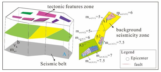
Figure 1.
Sketch Map of an earthquake activity model in China—a tri-class seismic source model.
Based on the basic assumptions and seismic activity parameters of the Chinese ground motion parameter zoning map, the following steps can be used to synthesize the seismic event set:
- (1)
- Youngs and Coppersmith [39] propose the exponential magnitude probability distribution approach to deal with the possible maximum () and minimum () magnitudes, as expressed in Equation (4). Based on the basic assumptions of Chinese probabilistic seismic hazard analysis, in the seismic belt, the magnitude distribution of earthquakes satisfies the doubly-truncated Gutenberg-Richter recurrence relation Equation (4) expressed below.
The value of is monotonous in [0, 1]. Let (r follows uniform distribution in [0, 1]). We can obtain Equation (5) through the inversion transformation of Equation (4).
Therefore, given a random number r from [0, 1], the magnitude of the earthquake can be determined (Figure 2) according to Equation (5).
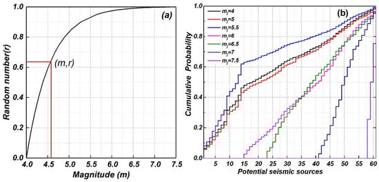
Figure 2.
Cumulative distribution function (a): Magnitude Cumulative Distribution Function. (b) the cumulative probability curves of potential sources under different magnitudes (mj).
- (2)
- The seismic activity in the seismic province follows the Poisson distribution [37]. In [0, t], the probability of a total of earthquakes will be observed, as shown in Equation (6).
We can acquire the cumulative distribution function of Equation (6) as shown in Equation (7):
The value of is continuity and monotonicity, and thus we can get the value of k through the DST.
If is set to the original time of an earthquake, the time interval of adjacent earthquakes (=) follows the exponential distribution [40], as shown in Equation (8):
According to the DST, the time interval of the earthquake event can be obtained. Let , then, the sequence of earthquake events can be obtained.
- (3)
- Determination of the location of the epicenter. The non-uniform spatial distribution of earthquake activity within the seismic belt is manifested by the activity of earthquakes at the potential source (which consists of the background seismicity zone and the tectonic features zone). In practice, the magnitude (m) is divided into intervals, and () represent the mid-value of the magnitude interval . The spatial distribution function () implies the occurrence probability of an earthquake generated by an individual potential source l with a magnitude interval mj.
According to the value of the , we can obtain the cumulative distribution function, as shown in Equation (9)
The value of is monotonous between [0, 1].
r follows a uniform distribution in [0, 1]. With the same method as the DST, given the random value r, the value of , can be determined according to Equations (9) and (10). For example, Figure 2b shows the spatial cumulative distribution function of the Liupanshan-Qilianshan seismic belt. The Liupanshan-Qilianshan seismic belt refers to a seismic zone in China that spans the Liupanshan Mountains and Qilianshan Mountains. These mountain ranges are located in the north-central part of the country. The seismic belt is characterized by tectonic activity, including the interaction of the Eurasian Plate and the Indian Plate. This geological region is known for its seismicity and has experienced earthquakes over the years. The graph’s horizontal axis provides a unique number for every background seismicity zone and tectonic feature zone, and the vertical axis shows the value of . According to Equations (9) and (10), given the random value r, the value of , which represents the number of can be determined.
Within the background seismicity zone and tectonic feature zone, the earthquake activity is supposed to be uniform. In order to generate the epicenter, we build up the minimal bounding rectangle of every background seismicity zone and tectonic feature zone and subsequently generate a two-dimensional random number (, ) that follows a uniform distribution between 0 and 1. According to Equations (11) and (12), we can obtain the point within the minimal bounding rectangle. If the point is located in the background seismicity zone or tectonic feature zone, it is considered the epicenter (Figure 3).
where and are respectively the maximum and minimum longitudes of the minimal bounding rectangle, and and are the maximum and minimum latitudes of the minimal bounding rectangle, respectively.
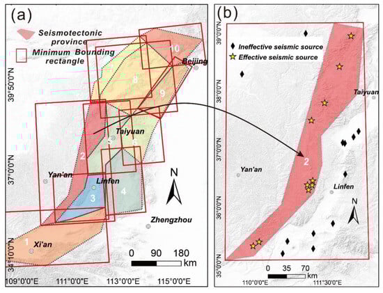
Figure 3.
The sketches of earthquake epicenter generation; (a) the potential sources of the Fenwei belt; (b) the local sketches of the distribution of the non-epicenter samples and epicenter samples based on background seismicity zone.
- (4)
- The seismic azimuth angle (θ) is established by sampling the probability function associated with the long-axis azimuth of potential source region attenuation. By taking into account the comprehensive influence of seismic belts on the site, we iteratively execute these procedures until the specified number of earthquakes is met within the seismic belt, completing a sampling cycle. Consequently, seismic event sets can be generated through extensive sampling simulations.
- (5)
- The conversion of latitude and longitude coordinates to Cartesian coordinates is performed for each earthquake within the event set. Using the epicenter as the coordinate origin, a Cartesian right-handed rectangular coordinate system is established, with the x-axis pointing to the true east and the y-axis pointing to the true north. This coordinate system undergoes a counterclockwise rotation by a specific angle (θ). The coordinates of the site in the new Cartesian coordinate system, denoted as (), can be determined through simultaneous equations, as illustrated in Equation (13).
Utilizing the iterative method [41] to solve the transcendental equation enables the determination of intensity values. Furthermore, the normalized residual (ε) is typically assumed to follow a normal distribution with a mean of zero and a standard deviation (σ). By incorporating ε into the intensity, the final intensity can be obtained. Considering the potential influence of all seismic zones on the site, the process is continued until the specified number of earthquakes is reached within the seismic zone, completing a sampling cycle. Subsequently, through large-scale sampling simulations, seismic event sets can be generated.
2.3. Estimation of Occurrence Probability of Earthquake Intensity
Based on the Monte Carlo method, for a site , our goal is to predict the probability of the seismic intensity exceeding specified seismic intensity in T years. represents the number of earthquake catalog groups simulated in the forthcoming T years. The number of simulated earthquake events in the g-th group is denoted as and the ground motion generated by the i-th earthquake event on the site is .
The total number affected by earthquake magnitude during T years is:
The number of ground motions () which is greater than and less than is shown in Equation (15).
Then, in T years and within the influence range of the site s, an earthquake with m occurs, and the probability that the ground motion value is greater than and less than is shown in Equation (16).
In T years, the mean rate of earthquake intensity occurrence at site s is shown in Equation (17).
In T years, the average number of earthquakes () with a magnitude of is shown in Equation (18).
Therefore, the occurrence probability of earthquake intensity () in T years is shown in Equation (19):
2.4. Estimation of Exceedance Probability of Earthquake Intensity
Based on the Monte Carlo method, in the g-th random independent repeat test, the maximum value of the ground motion generated by events on the site s is:
The number of ground motions that is greater than the set value and less than is written as:
Correspondingly, the extreme probability of the intensity of the specified seismic intensity () in T years is:
MCPSHA represents a relatively straightforward approach for seismic hazard assessment, depicted schematically in Figure 4. The program comprises three modules: (1) simulating earthquake catalog generation based on seismicity parameters; (2) calculating ground motion at the designated site; and (3) determining ground motion probability at the site.
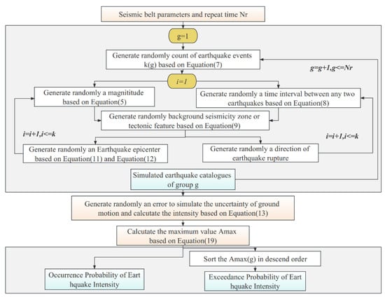
Figure 4.
Flowchart summarizing the method.
3. Geological Setting and Seismic Activity Parameters
Baoji City, situated in Shaanxi Province, is encompassed by the Loess Plateau, Qinling Mountain, and Weihe Basin (Figure 5). The Weihe River traverses the region from west to east. The Baoji area is influenced by three tectonic units, namely the QinLing fold belt, the Fen-Wei fault-depression zone, and the southern margin of the Ordos block [42]. Extensive seismic events have been recorded in this locale, with data sourced from the Catalogue of Shaanxi Earthquakes, 1189BC-2001AD (2015) (http://news.ceic.ac.cn/index.html?time=1524648589, accessed on 13 May 2019). Figure 5 shows the historical earthquake distribution around the Baoji area, spanning from 780 BC to 2015 AD. Notably, since 1973, the region has experienced numerous moderate and small earthquakes characterized by periodicity, migration, and recurrence.
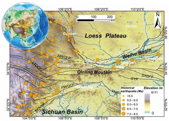
Figure 5.
Map depicting the topography, tectonic settings, and historical earthquakes (within 150 km around Baoji city from 870AD to 2015) distribution in the Baoji area. HYF: the Haiyuan fault; NWQLF: the North Margin of West Qinling fault; LTDCF: the Lintan-Dangchang fault; PWQCF: the Pingwu-Qingchuan fault; MJF: the Minjiang fault; BCYXF: the Beichuan-Yingxiu fault; SYF: the Shanyang fault; SXDFF: the Shangxian-Danfeng fault.
A total of 7 seismic belts may affect the Baoji area. In each background seismicity zone, tectonic feature zones are recognized and classified (Figure 6). The seismic activity parameters and the upper limit of magnitude for each seismic belt are measured based on the results of the “seismic microzonation of 4 cities in the Guan-Zhong” project (Figure 6). The background seismicity zone and tectonic feature zone parameters are obtained based on the results of the 5th National Seismic Zoning Map of China [43]. Seismic motion attenuation relations are based on the results of the “seismic microzonation of four cities in the Guan-Zhong” project (Figure 7) [44,45].
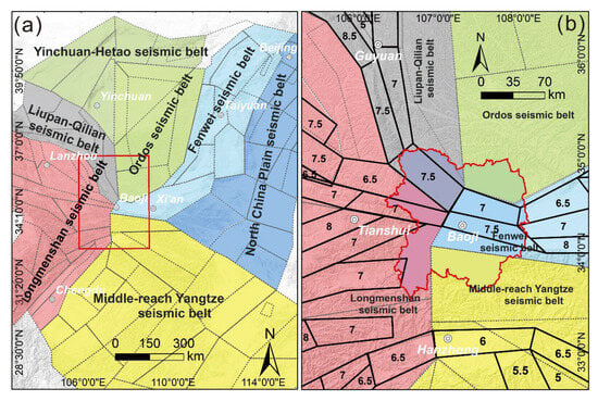
Figure 6.
Distribution of seven seismic belts in the study area. (a) seismic belts and background seismicity zones; and (b) potential seismic sources around the Baoji area. The red border represents the research area.
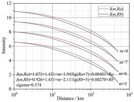
Figure 7.
Seismic motion attenuation relations in the Guan-Zhong area ( and are the semi-major axis and semi-minor axis of an ellipse, respectively).
4. Results and Analyses
4.1. Earthquake Catalog Simulation
To assess whether the generated seismic catalog adheres to the predefined seismic activity parameters and satisfies the assumed Poisson distribution hypothesis, we individually tabulate the annual occurrences of earthquakes with a magnitude of 4 or higher for each catalog group. A total of 50 samples (T = 50 years) were obtained. In the case of seismic events occurring times , the probability density of earthquake occurrences per year is calculated.
Figure 8 presents the Poisson distribution fitting of annual earthquake occurrences with a magnitude of 4 or higher, obtained through nonlinear fitting methods, based on four sets of simulated seismic catalogs from the Fenwei seismic zone (T = 50 years).
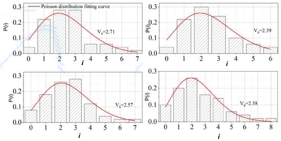
Figure 8.
Poisson distribution fitting diagram (four groups of sub-catalogues generated according to the seismic parameters of the Fenwei seismic province).
We compute the and b values for each subgroup of earthquake catalogs following the aforementioned procedure and then determine the mean values for each seismic belt. Figure 9 illustrates the parameters for the seven seismic belts obtained through simulation tests, while Table 1 provides details on the error parameters. The findings indicate that a sufficient number of repetitions guarantees the accuracy of the parameters.
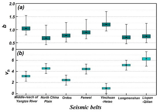
Figure 9.
Parameter test of the simulated earthquake catalogue ((a) b-value distribution of each simulated earthquake catalogue in different seismic belts, (b) Vh distribution of each simulated earthquake catalogue in different seismic belts).

Table 1.
Simulation catalogs (1,000,000 groups) of and b value test parameter.
4.2. Estimation of the Probability of an Earthquake Intensity
Using the method described in this paper, 1,000,000 groups of simulated earthquake catalogs over the next 50 years are generated. Figure 10 shows the distribution of earthquake epicenters (5.0 ≤ M ≤ 8.5) in 1 group of simulated earthquake catalogues in the next 50 years.
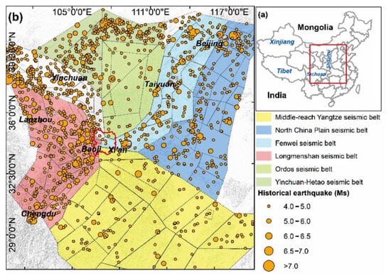
Figure 10.
The distribution of earthquake epicenters (5.0 ≤ M ≤ 8.5) in 1 group of simulated earthquake catalogues in the next 50 years. (a) Distribution of research area scope. (b) The distribution of earthquake epicenters in 1 group and spatial distribution maps of seismic zones.
Using a grid size of 0.05° × 0.05°, we compute the seismic intensity for the Baoji area at a specific hazard level. Macro-seismic intensity uncertainty is randomly drawn from a distribution with a mean of zero and a standard deviation of 0.574, truncated at two standard deviations. Figure 11 illustrates the mean intensity incidence rates for VI, VII, and VIII sites in the region over 50 years based on Equation (18). The results reveal the lowest incidence rate in the northeast and the highest in the northwest. One contributing factor may be the presence of more tectonic feature zones with a muz greater than 7.5 in the northwest, as compared to the northeast and southeast of Baoji city.
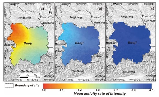
Figure 11.
The mean activity rate of intensity equals VI, VII, and VIII in the region in 50 years. ((a) the mean activity rate of intensity equals VI; (b) the mean activity rate of intensity equals VII; (c) the mean activity rate of intensity equals VIII).
Figure 12 displays the variation in intensity with the probability of occurrence and exceedance over 50 years in the region, calculated using our program. Notably, the difference between the two probabilities is more pronounced at intensity levels VI~VII, whereas at intensity level VIII, the difference is smaller.
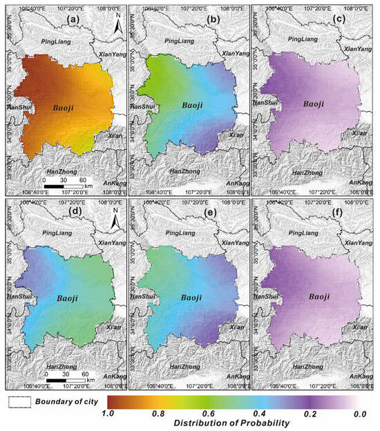
Figure 12.
Different intensity with probability in 50 years. (a–c) show the intensity VI, VII, and VIII with the probability of occurrence in the region; (d–f) display the intensity VI, VII, and VIII with the probability of exceedance in the region.
Figure 13 illustrates a comparison of the mean curves for the two probabilities (VI, VII, and VIII) in the region. The results reveal that as the intensity value increases, the disparity between the two gradually diminishes. Baoji is categorized as a moderate earthquake area, where occurrences of intensity above VIII are infrequent, and the occurrence probability of the intensity aligns closely with the extreme probability of the intensity value. However, in seismic loss estimation, specific regions necessitate individualized analysis owing to their diverse tectonic environments to determine their fundamental consistency. Despite minor distinctions, these differences may still introduce deviations in the evaluation results. Therefore, in the context of general seismic damage loss estimation, the exceedance probability of intensity cannot substitute for the occurrence probability of intensity.
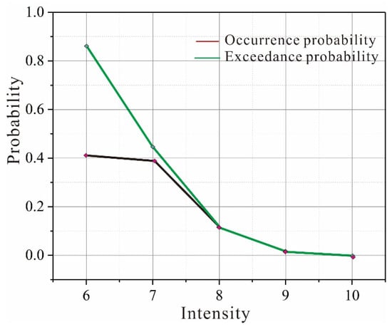
Figure 13.
Comparison of the two probabilities for each intensity in the region.
5. Discussion
To verify the accuracy of the results generated by our program, 300 points are randomly chosen in the Baoji area, and the hazard (return period T = 476 years) for each site is computed using both the traditional CPSHA method and the MCPSHA program (shown in Figure 14). Although the results from both methods exhibit similarities, some differences persist (Figure 14). The correlation between the two intensity results is high, at 0.98 (Figure 15a). To further assess the disparity between the CPSHA and MCPSHA results, we calculate the difference by subtracting the two outcomes (Figure 15b). The average difference is 0.16, with a minimum of 0.08, a maximum of 0.2, and a standard deviation of 0.03. The observed difference may stem from the excessive discretization employed by the CPSHA program, specifically in variables such as earthquake magnitude and epicenter distance, intended for simplified integration. In MCPSHA, the utilization of the Monte Carlo method based on Bayer’s large number theorem ensures that, with an ample number of random simulations, the frequency of events precisely reflects the probability of their occurrence. Additionally, a comprehensive series of repeated experiments assures the occurrence of all possible conditions. Consequently, as the number of simulations increases, even events with low probability are taken into account.
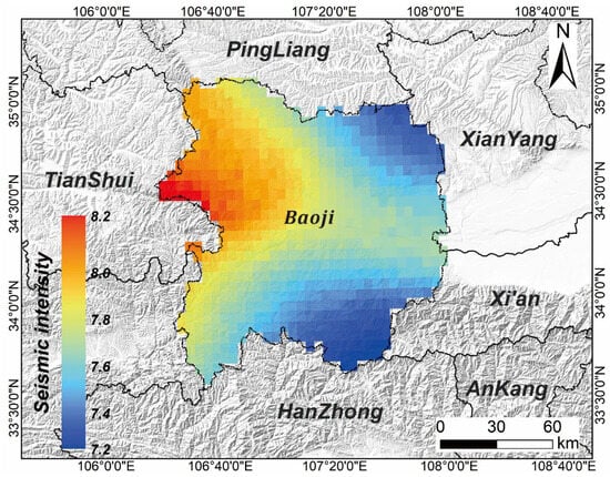
Figure 14.
Seismic hazard maps for 10% probability of exceedance in 50 years calculated by MCPSHA (T = 476 years return period).
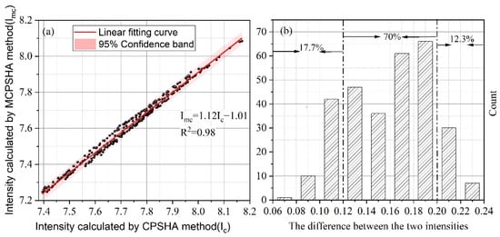
Figure 15.
Comparison of MCPSHA and CPSHA intensity fitting results (T = 476-year return period). (a) The correlation between the two intensity results. (b) Statistical chart of the difference between two results.
The most appropriate and scientifically sound approach for validating the results of the PSHA method is to rely on historical data specific to the region. The seismic activity history spanning approximately 3000 years in the studied area serves as a valuable validation tool. We have presented the expected occurrence probability for a mean return period of 476 years, a period that repeats more than six times within the historical information of the region. However, due to a lack of data, we were unable to locate several or a few sites with recorded macroseismic intensities. In future research, we intend to compare the modeling of observed intensity occurrences with those estimated by MCPSHA. Such a comparison is sufficient to either substantiate or negate the robustness of the proposed methodology.
The current seismic hazard analysis method is generally utilized for engineering seismic fortification; thus, only the extreme intensity of the site is taken into consideration. This method is not applicable to earthquake damage estimation [46,47]. The seismic loss of a site is not only caused by an earthquake, which corresponds to its extreme intensity. Although the original extreme value (only considering one maximum case) correctly handles the randomness of future earthquake occurrences, if the duration is long and the site is located in a region with frequently occurring strong earthquakes, the loss caused by multiple earthquakes with the same intensity and that associated with one earthquake may obviously differ [48]. Therefore, when calculating the expected earthquake-induced loss, both the occurrence probability and the occurrence frequency of the seismic intensity should be considered. For example, the site may suffer multiple VI-intensity ground motions within a given number of years, and the loss produced in this situation is twice that generated by an earthquake with an intensity of VI. The estimation method based on extreme intensity ignores the above effects. Therefore, the seismic hazard analysis method of the engineering site cannot be directly used.
Both the probability of occurrence and exceedance are important indicators of seismic hazards for a given site, but the meaning of the two indicators is distinctly different. Furthermore, the exceedance probability itself contains the meaning of extreme intensity. For any site, it is assumed that the frequency of strong earthquakes will be extremely high in the next 50 years, and the possibility of earthquakes with a magnitude of around 6 is very high (even more earthquakes with a magnitude less than 6). Under this assumption, it is almost inevitable that the site will be affected by intensities VI and VII within a given number of years. The occurrence probability of intensity VI is high, but the probability of intensity VI as an extreme value is relatively small (Figure 12). The method of subtraction adjacent exceedance probability within a given period of time can be considered the exceedance probability of the extreme intensity at the site within a specified number of years. Numerically, it is lower than the occurrence probability of the intensity (Figure 13). From a statistical point of view, if the extreme intensity is a fixed value, the probability of the site being affected is zero. There are two possibilities in this situation: The first is that the intensity values that affect the site are all less than the fixed value within a given period of time; the second is that the probability of an extreme intensity value in a given period of time is 100% equal to 1 (i.e., it is inevitable). In the second case, although the subtraction adjacent exceedance probability is zero, the probability that the intensity will affect the site may be large. Therefore, the exceedance probability of intensity cannot be used to replace the occurrence probability of intensity.
The Monte Carlo method poses computational challenges, particularly for intricate seismic models, leading to high computational costs due to the necessity for an extensive number of random simulations. Moreover, the accuracy of the method hinges on both the quantity and quality of random sampling; insufficient or inappropriate sampling could introduce biases to the results. In the seismic zone earthquake simulation of this study, the Poisson model employed for earthquake occurrence times often deviates from real seismic activity, typically following a clustered model. Addressing the issue of mutual triggering between earthquakes (such as Poisson + clustering), future research can refine the sampling function and incorporate a seismicity model (e.g., ETAS) to yield more precise results, especially in regions with limited historical earthquake records and complex geological structures. Meanwhile, Bolotin [25] systematically investigates random factors in seismic risk assessment for structures, discussing the randomization of key parameters in numerical simulations and applying asymptotic distributions of extremes for more reliable estimates in rare seismic events with multiple response restrictions. In this study, the uniform setting of key parameters, such as seismic intensity attenuation, to a single value using the Monte Carlo method in tandem with spatiotemporal heterogeneous seismic hazard analysis in China may impact the accuracy of the seismic hazard analysis results.
6. Conclusions
In this paper, we derived the formula for the occurrence probability of earthquake intensity and the mean rate of earthquake intensity occurrence within a specified time period, and we have developed a program named MCPSHA. The three fundamental components of MCPSHA are carefully considered, including the seismic source model, magnitude recurrence model, and ground motion attenuation model. This approach offers greater flexibility and transparency, making it easily adaptable to modifications in the seismicity model. For instance, the introduction of complex seismic activity models requires minimal reprogramming—only a new probability density function (pdf) function needs to be provided. Additionally, the modeling of uncertainty in input parameters is highly flexible, accomplished solely through the use of a standard deviation rather than relying on the discrete branches of a logic tree.
Over the next 50 years, we will investigate the disparity between occurrence probability and extreme probability (i.e., the difference in exceeding probability, often used as a substitute for occurrence probability) in the Baoji area. The findings reveal that, for intensities within VI~VII, the difference is nearly twofold, gradually diminishing with increasing intensity. This study underscores that exceeding probability and occurrence probability for specific intensities cannot be interchangeable. Accurate seismic intensity occurrence probability stands as a crucial foundation for seismic risk analysis and loss estimation.
Author Contributions
Conceptualization, X.W. and X.S.; methodology, X.W. and X.S.; software, X.S.; validation, X.W. and X.S.; formal analysis, X.S. and C.X.; data curation, X.W. and X.S.; writing original draft preparation, X.W., X.S. and S.M.; writing—review and editing, X.W., X.S. and C.X.; supervision, C.X.; project administration, X.W. and C.X.; funding acquisition, C.X. All authors have read and agreed to the published version of the manuscript.
Funding
This work was funded by the National Institute of Natural Hazards, the Ministry of Emergency Management of China (ZDJ2021–12), and the National Natural Science Foundation of China (41941016), and the National Key Research and Development Program of China (2021YFB3901205).
Institutional Review Board Statement
Not applicable.
Informed Consent Statement
Not applicable.
Data Availability Statement
The data presented in this study are available on request from the corresponding author. The data are not publicly available due to privacy.
Acknowledgments
Thanks are given for the provision of seismicity characteristics from the Institute of Geophysics, China Earthquake Administration.
Conflicts of Interest
The authors declare no conflict of interest.
References
- Li, Y.; Zhang, Z.; Xin, D. A Composite Catalog of Damaging Earthquakes for Mainland China. Seismol. Res. Lett. 2021, 92, 3767–3777. [Google Scholar] [CrossRef]
- Liu, J.; Wang, Z.; Xie, F.; Lv, Y. Seismic hazard assessment for greater North China from historical intensity observations. Eng. Geol. 2013, 164, 117–130. [Google Scholar] [CrossRef]
- Zhu, W.; Liu, K.; Wang, M.; Koks, E.E. Seismic Risk Assessment of the Railway Network of China’s Mainland. Int. J. Disaster Risk Sci. 2020, 11, 452–465. [Google Scholar] [CrossRef]
- Cornell, C.A. Engineering seismic risk analysis. Bull. Seismol. Soc. Am. 1968, 58, S183–S188. [Google Scholar] [CrossRef]
- Tanyas, H.; Rossi, M.; Alvioli, M.; Westen, C.J.; Marchesini, I. A global slope unit-based method for the near real-time prediction of earthquake-induced landslides. Geomorphology 2019, 327, 126–146. [Google Scholar] [CrossRef]
- Crowley, H.; Despotaki, V.; Rodrigues, D.; Silva, V.; Toma-Danila, D.; Riga, E.; Karatzetzou, A.; Fotopoulou, S.; Zugic, Z.; Sousa, L.; et al. Exposure model for European seismic risk assessment. Earthq. Spectra 2020, 36, 875529302091942. [Google Scholar] [CrossRef]
- Silva, V.; Amo-Oduro, D.; Calderon, A.; Costa, C.; Dabbeek, J.; Despotaki, V.; Martins, L.; Pagani, M.; Rao, A.; Simionato, M.; et al. Development of a Global Seismic Risk Model. Earthq. Spectra 2020, 36, 372–394. [Google Scholar] [CrossRef]
- Silva, V.; Crowley, H.; Varum, H.; Pinho, R. Seismic risk assessment for mainland Portugal. Bull. Earthq. Eng. 2015, 13, 429–457. [Google Scholar] [CrossRef]
- Dolce, M.; Prota, A.; Borzi, B.; da Porto, F.; Lagomarsino, S.; Magenes, G.; Moroni, C.; Penna, A.; Polese, M.; Speranza, E.; et al. Seismic risk assessment of residential buildings in Italy. Bull. Earthq. Eng. 2021, 19, 2999–3032. [Google Scholar] [CrossRef]
- Mcguire, R.K. Deterministic vs. probabilistic earthquake hazards and risks. Soil Dyn. Earthq. Eng. 2011, 21, 377–384. [Google Scholar] [CrossRef]
- Milner, K.R.; Shaw, B.E.; Goulet, C.A.; Richards-Dinger, K.B.; Callaghan, S.; Jordan, T.H.; Dieterich, J.H.; Field, E.H. Toward Physics-Based Nonergodic PSHA: A Prototype Fully Deterministic Seismic Hazard Model for Southern California. Bull. Seismol. Soc. Am. 2021, 111, 898–915. [Google Scholar] [CrossRef]
- Valentini, A.; Pace, B.; Boncio, P.; Visini, F.; Pagliaroli, A.; Pergalani, F. Definition of Seismic Input From Fault-Based PSHA: Remarks After the 2016 Central Italy Earthquake Sequence. Tectonics 2019, 38, 595–620. [Google Scholar] [CrossRef]
- Taroni, M.; Akinci, A. Good practices in PSHA: Declustering, b-value estimation, foreshocks and aftershocks inclusion; a case study in Italy. Geophys. J. Int. 2020, 224, 1174–1187. [Google Scholar] [CrossRef]
- Slejko, D.; Rebez, A.; Santulin, M. Seismic hazard estimates for the Vittorio Veneto broader area (NE Italy). Boll. Geofis. Teor. Appl. 2008, 49, 329–356. [Google Scholar]
- D’Amico, V.; Albarello, D. SASHA: A Computer Program to Assess Seismic Hazard from Intensity Data. Seismol. Res. Lett. 2008, 79, 663–671. [Google Scholar] [CrossRef]
- Turkstra, C. Seismic Risk and Engineering Decisions; Elsevier Scientific Pub. Co.: Amsterdam, The Netherlands, 1976; pp. 287–289. [Google Scholar]
- Yuan, H.; Gao, X.; Qi, W. Assessing the seismic risk of cities at fine-scale: A case study of Haidian District in Beijing, China. Seismol. Geol. 2016, 38, 197–210. [Google Scholar]
- Chen, Y.; Chen, Q.; Chen, L. Vulnerability analysis in earthquake loss estimate. Nat. Hazards 2001, 23, 349–364. [Google Scholar]
- Peresan, A.; Magrin, A.; Nekrasova, A.; Kossobokov, V.G.; Panza, G.F. Earthquake recurrence and seismic hazard assessment: A comparative analysis over the Italian territory. In Proceedings of the Earthquake Resistant Engineering Structures IX, Coruña, Spain, 8–10 July 2013; pp. 23–34. [Google Scholar]
- Fu, Z.; Jiang, L.; Wang, X. Non-Stationary Poisson process of earthquake occurrence and research on long-and medium-term probabilistic earthquake prediction. Earthquake 1998, 18, 105–111. (In Chinese) [Google Scholar]
- Parsons, T. Monte Carlo method for determining earthquake recurrence parameters from short paleoseismic catalogs: Example calculations for California. J. Geophys. Res. 2008, 113, B03302. [Google Scholar] [CrossRef]
- Bourne, S.J.; Oates, S.J.; Bommer, J.J.; Dost, B.; Elk, J.v.; Doornhof, D. A Monte Carlo Method for probabilistic hazard assessment of induced seismicity due to conventional natural gas production. Bull. Seismol. Soc. Am. 2015, 105, 1721–1738. [Google Scholar] [CrossRef]
- Mohammed, T.; Atkinson, G.M.; Assatourians, K. Uncertainty in recurrence rates of large magnitude events due to short historic catalogs. J. Seismol. 2014, 18, 565–573. [Google Scholar] [CrossRef]
- Musson, R.M.W. The use of Monte Carlo simulations for seismic hazard assessment in the U.K. Ann. Geophys. 2000, 43, 1–9. [Google Scholar] [CrossRef]
- Bolotin, V. Seismic risk assessment for structures with the Monte Carlo simulation. Probabilistic Eng. Mech. 1993, 8, 169–177. [Google Scholar] [CrossRef]
- Emmi, P.C.; Horton, C.A. A Monte Carlo simulation of error propagation in a GIS-based assessment of seismic risk. Int. J. Geogr. Inf. Syst. 1995, 9, 447–461. [Google Scholar] [CrossRef]
- Musson, R.M.W.; Sellami, S.; Brüstle, W. Preparing a seismic hazard model for Switzerland: The view from PEGASOS Expert Group 3 (EG1c). Swiss J. Geosci. 2009, 102, 107–120. [Google Scholar] [CrossRef][Green Version]
- Gaxiola-Camacho, J.R.; Azizsoltani, H.; Villegas-Mercado, F.J.; Haldar, A. A novel reliability technique for implementation of performance-based seismic design of structures. Eng. Struct. 2017, 142, 137–147. [Google Scholar] [CrossRef]
- Assatourians, K.; Atkinson, G.M. EqHaz: An Open-Source Probabilistic Seismic-Hazard Code Based on the Monte Carlo Simulation Approach. Seismol. Res. Lett. 2013, 84, 516–524. [Google Scholar] [CrossRef]
- Weatherill, G.A. A Monte Carlo Approach to Probabilistic Seismic Hazard Analysis in the Aegean Region. Tectonophysics 2009, 492, 253–278. [Google Scholar] [CrossRef]
- Liu, J.; Gao, M.; Wu, S. Probabilitic seismic landslide hazard zonation method and its application. Chin. J. Rock Mech. Eng. 2016, 35, 3100–3110. [Google Scholar]
- Li, B.; Sørensen, M.B.; Atakan, K.; Li, Y.; Li, Z. Probabilistic Seismic Hazard Assessment for the Shanxi Rift System, North China. Bull. Seismol. Soc. Am. 2020, 110, 127–153. [Google Scholar] [CrossRef]
- Li, C.; Xu, W.; Wu, J.; Gao, M. Time-dependent probabilistic seismic hazard assessment for Taiyuan, Shanxi Province, China, and the surrounding area. J. Seismol. 2017, 21, 749–757. [Google Scholar] [CrossRef]
- Huh, U.; Cho, W.; Ramachandra, R.; Joy, D.C. Monte Carlo Modeling of Ion Beam Induced Secondary Electrons. Microsc. Microanal. 2016, 168, 28. [Google Scholar] [CrossRef]
- Matsumoto, M.; Nishimura, T. Monte Carlo and Quasi-Monte Carlo Methods 2000. Acta Numer. 1998, 7, 1–49. [Google Scholar]
- Matsumoto, M.; Nishimura, T. Mersenne twister: A 623-dimensionally equidistributed uniform pseudo-random number generator. Acm Trans. Model. Comput. Simul. 1998, 8, 3–30. [Google Scholar] [CrossRef]
- Pan, H.; Gao, M.; Xie, F. The Earthquake Activity Model and Seismicity Parameters in the New Seismic Hazard Map of China. Technol. Earthq. Disaster Prev. 2013, 8, 11–23. [Google Scholar]
- Pan, H.; Gao, M.; Li, J. Comments on the Models of Seismic Source and Parameters Used in the New Edition of United States National Seismic Hazard Maps. Technol. Earthq. Disaster Prev. 2009, 4, 131–140. [Google Scholar]
- Youngs, R.R.; Coppersmith, K.J. Implications of fault slip rates and earthquake recurrence models to probabilistic seismic hazard estimates. Bull. Seismol. Soc. Am. 1985, 75, 939–964. [Google Scholar] [CrossRef]
- Hu, Y. Earthquake Engineering; Seismological Press: Beijing, China, 2006; p. 566. [Google Scholar]
- Lanczos, C. An Iteration Method for the Solution of the Eigenvalue Problem of Linear Differential and Intergral Operators. J. Res. Natl. Bur. Stand. 1950, 45, 255–282. [Google Scholar] [CrossRef]
- Shi, J.; Wu, L.; Wu, S.; Li, B.; Wang, T.; Xin, P. Analysis of the causes of large-scale loess landslides in Baoji, China. Geomorphology 2016, 264, 109–117. [Google Scholar] [CrossRef]
- Zhou, B.; Chen, G.; Gao, Z.; Zhou, Q.; Li, J. The technical highlights in identifying the potential seismic sources for the update of national seismic zoning map of China. Technol. Earthq. Disaster Prev. 2016, 8, 113–124. [Google Scholar]
- Fan, W.; Du, W.; Wang, X.; Shao, H.; Wen, Y. Seismic motion attenuation relations in shaanxi areas. J. Earthq. Eng. Eng. Vib. 2011, 31, 47–54. [Google Scholar]
- Chen, D. Study on relationship between ground-motion peak accelerations and different levels of exceeding probability in Guanzhong area of Shaanxi province. J. Earthq. Eng. Eng. Vib. 2012, 32, 34–40. [Google Scholar] [CrossRef]
- Gao, M. Occurrence probability model of earthquke intensity based on the Poisson distribution. Earthq. Res. China 1996, 13, 195–201. [Google Scholar]
- Chen, K.; Gao, M. Computational Method of Occurrence Probability of Earthquake Intensity Based on MapInfo. Earthq. Res. China 2008, 24, 399–406. [Google Scholar]
- Mulargia, F.; Stark, P.B.; Geller, R.J. Why is probabilistic seismic hazard analysis (PSHA) still used? Phys. Earth Planet. Inter. 2017, 264, 63–75. [Google Scholar] [CrossRef]
Disclaimer/Publisher’s Note: The statements, opinions and data contained in all publications are solely those of the individual author(s) and contributor(s) and not of MDPI and/or the editor(s). MDPI and/or the editor(s) disclaim responsibility for any injury to people or property resulting from any ideas, methods, instructions or products referred to in the content. |
© 2024 by the authors. Licensee MDPI, Basel, Switzerland. This article is an open access article distributed under the terms and conditions of the Creative Commons Attribution (CC BY) license (https://creativecommons.org/licenses/by/4.0/).