Model-Free Adaptive Control of an Active Half-Vehicle-Seat System Coupled with a Nonlinear Energy Sink Inerter (NESI)

Abstract

In order to reduce vehicle vibration and improve vehicle ride comfort and handling stability, a nonlinear energy sink inerter (NESI) is designed by combing an inerter and nonlinear energy sink (NES) for use in the seat suspension and vehicle suspension for the half-vehicle-seat (HVS) system; furthermore, a model-free adaptive control (MFAC) method based on the genetic algorithm is proposed to enhance the dynamic performance of the passive HVS system. The dynamic model of the active HVS system coupled with NESI using the MFAC method is established; its dynamic responses under pavement random and shock excitations are acquired using the numerical method and the dynamic performance is evaluated by seven evaluation indicators. The efficacy of the MFAC method is demonstrated through comparative analysis with the original passive HVS system, the HVS system coupled with NESI, and the active HVS system coupled with NESI using the proportional integral derivative (PID) control method. In addition, the influence of the installed position of MFAC on the dynamic performance of the active HVS system coupled with NESI is examined. The results show that for the active HVS system coupled with NESI using the MFAC method, compared with the other three HVS systems, the root mean square (RMS) values of the vehicle body vertical acceleration, vehicle body pitch acceleration, seat vertical acceleration, and front and rear suspension dynamic travel under pavement random excitation are smaller, the corresponding peak amplitudes under pavement shock excitation reduce, and the vibration attenuation time shortens; the RMS values of the front and rear dynamic tire loading under pavement random excitation are slightly smaller, the corresponding peak amplitudes under pavement shock excitation increase, and the vibration attenuation time decreases, which reflects the best dynamic performance among the four HVS systems and shows the effectiveness of the MFAC method. Furthermore, the control effect of the MFAC method is the best when it acts both on the seat and vehicle suspensions.

1. Introduction

It is well known that the adverse vibrations caused by uneven pavement surfaces significantly affect passenger comfort and vehicle handling stability; severe vibrations can lead to dizziness, spinal disease, lumbar disc pain, and other diseases [1]. Passenger comfort is related to a variety of factors, such as the structure and material of the seat back and the vibration transmitted by the seat to the human body, among which the latter is closely related to the vehicle seat vertical acceleration, as well as the vehicle body vertical and pitch accelerations. The suspension system is one of the most critical components in a vehicle; it plays a crucial role in reducing adverse vibration and improving ride comfort during vehicle operation [2]. The suspension system primarily transfers and absorbs vibrations from the road surface via the shock absorber, thereby attenuating vehicle vibrations, stabilizing vehicle body posture, and enhancing ride comfort and vehicle stability under various road conditions [3]. Given that the vehicle seat is in direct contact with the human body, enhancing the vibration isolation performance of the seat suspension is crucial for reducing human body vibration and improving ride comfort, while adjustments to the structural parameters of the seat suspension have less impact on the other aspects of vehicle performance [4]. Therefore, improving the vibration attenuation performance of both the seat suspension and vehicle suspension is important in vehicle engineering.

In terms of analyzing the vehicle ride comfort, Li et al. [5] established a seven-degree-of-freedom (DOF) vehicle dynamic model and analyzed the vertical, pitch, and roll acceleration values of a heavy mine vehicle under full-load and no-load excitation on a class D road surface. Li et al. [6] analyzed and evaluated the changes in passenger comfort when drivers contact the pressure pad on the seat surface under different driving durations. In order to improve ride comfort under different pavement conditions, some scholars apply the adaptive control method to the vehicle suspension system. Palomares et al. [7] proposed an adaptive optimal control strategy to improve ride comfort by minimizing vertical body acceleration. Jinwoo et al. [8] proposed a suspension controller design method based on an adaptive feedforward algorithm to enhance ride comfort and reduce the heave and pitch vibration of sprung mass. Zhang et al. [9] designed a control method using the genetic algorithm to optimize the fuzzy proportional integral derivative (PID) control algorithm and studied the vehicle ride comfort of the vehicle suspension system by taking the vertical acceleration of the vehicle body, suspension deflection, and wheel dynamic load as evaluation criteria.

The nonlinear energy sink (NES) is an innovative vibration attenuation device and can absorb and dissipate the energy of the main structure [10]. Due to its superior vibration reduction performance, the NES has been widely applied in various fields, such as civil engineering [11,12,13], aerospace engineering [14,15,16], and vehicle engineering [17,18,19]. However, achieving optimal vibration suppression performance of the NES typically requires a larger mass, which contradicts the lightweight vehicle design principle. To address this challenge, a dual-end structural element, the inerter, has been developed to achieve a mass amplification effect, where the output force-to-relative acceleration ratio is termed as inertance [20]. Owing to the mass amplification effect of the inerter, researchers have replaced the mass block in the NES with an inerter, creating a new vibration suppression mechanism known as the nonlinear energy sink inerter (NESI) [21]. Zhang et al. [22] constructed a new type of NESI that successfully achieves ideal vibration damping performance with a smaller mass. Javidialesaadi and Wierschem [23] developed an innovative NESI configuration in which the inerter is positioned between the mass block and the stationary base of an NES, thereby significantly enhancing its effectiveness. Cao et al. [24] used an NESI to suppress the torsional vibration in the rotor system, which reduces the required rotary inertia for torsional vibration suppression. Sui et al. [25] conducted a detailed analysis of the response mechanism and damping effect of the NESI and studied how NESI parameters influence the system’s overall performance, particularly in terms of vibration suppression and stability under varying conditions. Wang et al. [26] applied an NESI in a vehicle suspension system to enhance its vibration damping performance under various pavement excitation levels.

In a previous study by the authors [27], the NESI was applied to the vehicle suspension and seat suspension in a half-vehicle-seat (HVS) system. The harmonic balance method and pseudo-arc length method were used to analyze the dynamic characteristic of the passive HVS system coupled with the NESI under pavement harmonic and random excitations, and the influence of the NESI’s structural parameters on the dynamic performance was analyzed. The results indicate that the NESI can reduce the resonance peak value of seat dynamic travel, front and rear suspension dynamic travel, and front and rear dynamic tire loading; however, seat vertical acceleration, vehicle body vertical acceleration, and pitch acceleration increase slightly. Although the application of the NESI in a passive HVS system improves vehicle vibration attenuation performance [27], its structural parameters are fixed and cannot adaptively adjust to changing road impacts. Compared with passive suspension, active suspension can adjust itself in real time based on information such as vehicle speed and road conditions, ensuring optimal suspension performance across various driving conditions. Du et al. [28] developed H∞ state feedback control to minimize human head acceleration through integrated control of the seat and vehicle suspension and designed a static output feedback controller for the unmeasured driver model during driving. To address the influence of human body dynamics and uncertainties in seat skeleton dynamics, Lathkar et al. [29] designed a sliding mode controller based on a disturbance observer and analyzed the dynamic performance of a 4-DOF human–seat model; the results indicate that the acceleration transmitted from the seat to the human body is significantly reduced. Han et al. [30] proposed a suspension control strategy based on the adaptive fuzzy PID control method to address uncertainties in road disturbances.

In summary, to mitigate the impact of unmodeled vehicle dynamic factors and driver dynamic interference during driving, some researchers employ sensors and feedback control, while others utilize fuzzy methods to address the uncertainty of road disturbances. Hou and Jin [31] proposed a data-driven model-free adaptive control (MFAC) method for multi-input multi-output nonlinear discrete-time systems, utilizing the concept of pseudo-partial derivatives and dynamic linearization. The primary feature of this method is that the controller design relies solely on the measured input/output (I/O) data of the controlled object. Analysis and extensive simulations demonstrate that the MFAC method ensures bounded input–bounded output (BIBO) stability and convergence of tracking errors. As of late, the MFAC method has been widely applied to complex nonlinear systems and systems that are challenging to model [32,33,34,35]. Building on the author’s previous work [27], this paper designs an MFAC method for the joint control of seat suspension and vehicle suspension, utilizes a genetic algorithm to optimize the controller parameters, and efficiently determines the optimal parameter combination. The efficacy of the MFAC method is investigated through comparative analysis with the original passive HVS system, an HVS system coupled with an NESI, and an active HVS system coupled with an NESI using the PID control method. In addition, the influence of the installed position of MFAC on the dynamic performance of the active HVS system coupled with NESI is examined.

The structure of this paper is outlined as follows: Section 2 introduces a dynamic model of an active HVS system coupled with an NESI and establishes its nonlinear dynamic equations using Newton’s second law. Section 3 presents the formulations of the MFAC method based on the genetic algorithm. Section 4 and Section 5 analyze the dynamic performance of the active HVS system coupled with an NESI using the MFAC method under random pavement and shock excitations, respectively, which provides a detailed analysis of the effect of the MFAC method on the dynamic performance of the HVS system. Section 6 provides a summary of the paper.

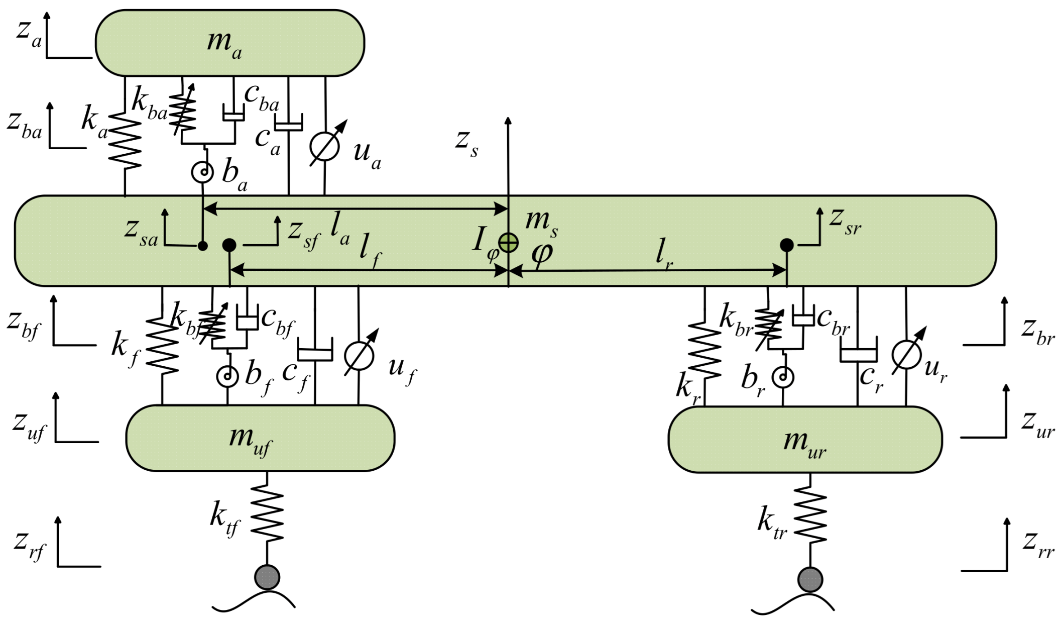
2. Active HVS System Coupled with NESI

Figure 1 presents the schematic diagram of an active HVS system coupled with NESI. m_s, m_uf, m_ur and m_a are the masses of the vehicle body, front tire, rear tire, and seat, respectively; I_φ is the body pitch moment of inertia; k_f, k_r, k_tf, k_tr and k_a are the stiffnesses of the front and rear suspensions, front and rear tires, and seat suspension, respectively; c_f, c_r, c_tf, c_tr and c_a represent the damping coefficients of the front and rear suspensions, front and rear tires, and seat suspension, respectively. l_f, l_r and l_a are the distances from the center of mass to the front axle, rear axle, and seat, respectively; b_f (b_r, b_a), k_bf (k_br, k_ba) and c_bf (c_br, c_ba) represent the inertance, cubic stiffness, and damping coefficients of the NESI installed between the vehicle body and the front and rear tires, and between the vehicle body and seat, respectively. φ is the body pitch angle; z_s, z_a, z_uf, z_ur, z_ba, z_bf and z_br denote the displacements of the vehicle body center of mass, seat center of mass, front and rear tires, the inerter of the NESI installed between the vehicle body and seat, and the inerters of the NESIs installed between the vehicle body and the front and rear tires, respectively. z_rf and z_rr represent the front and rear pavement excitations, respectively; u_a, u_f and u_r are the active forces acting on the seat suspension and front and rear suspensions, respectively. Table 1 presents the structural parameters of the active HVS system. The structural parameters of the NESIs are obtained in [27], which are the optimized structural parameters using the genetic algorithm. For the NESI installed between the vehicle body and seat, the structural parameters are b_a = 299.662 kg, k_ba = 3.25 × 10⁵ N/m, and c_ba = 634.83 Ns/m. For the NESIs installed between the vehicle body and the front and rear tires, the structural parameters are b_f = 86.7921 kg, b_r = 97.9515 kg, k_bf = 2.76414 × 10⁶ N/m, k_br = 1.25991 × 10⁶ N/m, c_bf = 504.536 Ns/m, and c_br = 616.126 Ns/m.

Figure 1. Active HVS system coupled with NESI.

Table 1. Structural parameters of the active HVS system coupled with NESI.

Parameter	Value	Parameter	Value	Parameter	Value
$m_s$	690 kg	$c_a$	800 Ns/m	$l_a$	1.4 m
$I_{\phi }$	1222 kgm2	$k_{tf}$	2 × 105 N/m	$l_r$	1.5 m
$m_{uf}$	45 kg	$k_{tr}$	2 × 105 N/m	$c_f$	1000 Ns/m
$m_{ur}$	45 kg	$k_f$	18,000 N/m	$c_r$	1000 Ns/m
$m_a$	80 kg	$k_r$	22,000 N/m
$k_a$	8000 N/m	$l_f$	1.3 m

Utilizing Newton’s second law, the dynamic equations for the active HVS system coupled with NESI are derived. These equations are formulated based on the static equilibrium positions of the vehicle body, seat, front and rear suspensions, NESI, and front and rear tires. The dynamic equation describing the vertical motion of the vehicle body is

$$\begin{array}{l}{m}_s{z}_s^{″}-b_a(z_{ba}^{″}-z_{sa}^{″})+c_f(z_{sf}^{\prime }-z_{uf}^{\prime })+c_r(z_{sr}^{\prime }-z_{ur}^{\prime })+c_a(z_{sa}^{\prime }-z_a^{\prime })+k_f(z_{sf}-z_{uf})+k_r(z_{sr}-z_{ur})\theta \\ +k_a(z_{sa}-z_a)+c_{bf}(z_{sf}^{\prime }-z_{bf}^{\prime })+c_{br}(z_{sr}^{\prime }-z_{br}^{\prime })+k_{bf}(z_{sf}-z_{bf}{)}^3+k_{br}(z_{sr}-z_{br}{)}^3-u_f-u_r-u_a=0\end{array}$$

(1)

The dynamic equation describing the pitch motion of the vehicle body is

$$\begin{array}{l}{I}_{\phi }{\phi }^{″}+c_r{l}_r(z_{sr}^{\prime }-z_{ur}^{\prime })-c_f{l}_f(z_{sf}^{\prime }-z_{uf}^{\prime })-c_a{l}_a(z_{sa}^{\prime }-z_a^{\prime })+k_r{l}_r(z_{sr}-z_{ur})-k_f{l}_f(z_{sf}-z_{uf})-\\ k_a{l}_a(z_{sa}-z_a)+b_a(z_{ba}^{″}-z_{sa}^{″})l_a+c_{br}{l}_r(z_{sr}^{\prime }-z_{br}^{\prime })-c_{bf}{l}_f(z_{sf}^{\prime }-z_{bf}^{\prime })+k_{br}{l}_r(z_{sr}-z_{br}{)}^3\\ -k_{bf}{l}_f(z_{sf}-z_{bf}{)}^3+l_f{u}_f-l_r{u}_r+l_a{u}_a=0\end{array}$$

(2)

The dynamic equation describing the front tire is

$$(m_{uf}+b_f)z_{uf}^{″}-b_f{z}_{bf}^{″}-c_f{z}_{sf}^{\prime }+c_f{z}_{uf}^{\prime }-k_f{z}_{sf}+(k_f+k_{tf})z_{uf}-u_f=k_{tf}{z}_{rf}$$

(3)

The dynamic equation describing the rear tire is

$$(m_{ur}+b_r)z_{ur}^{″}-b_r{z}_{br}^{″}-c_r{z}_{sr}^{\prime }+c_r{z}_{ur}^{\prime }-k_r{z}_{sr}+(k_r+k_{tr})z_{ur}-u_r=k_{tr}{z}_{rr}$$

(4)

The dynamic equation describing the vehicle seat is

$$m_a{z}_a^{″}+c_a(z_a^{\prime }-z_{sa}^{\prime })+k_a(z_a-z_{sa})+k_{ba}{(z_a-z_{ba})}^3+c_{ba}(z_a^{\prime }-z_{ba}^{\prime })-u_a=0$$

(5)

The dynamic equation describing the NESI installed between the vehicle body and seat is

$$b_a(z_b^{″}-z_{sa}^{″})-k_b{(z_a-z_b)}^3-c_b(z_a^{\prime }-z_b^{\prime })=0$$

(6)

The dynamic equation for the NESI installed between the vehicle body and the front tire is

$$b_f{z}_{bf}^{″}-b_f{z}_{uf}^{″}-c_{bf}{z}_{sf}^{\prime }+c_{bf}{z}_{bf}^{\prime }+k_{bf}{(z_{bf}-z_{sf})}^3=0$$

(7)

The dynamic equation for the NESI installed between the vehicle body and the rear tire is

$$b_r{z}_{br}^{″}-b_r{z}_{ur}^{″}-c_{br}{z}_{sr}^{\prime }+c_{br}{z}_{br}^{\prime }+k_{br}{(z_{br}-z_{sr})}^3=0$$

(8)

As shown in Figure 1, when the pitch angle of the vehicle body is small, the displacements z_sf, z_sr and z_sa can be approximated as

$$\begin{array}{ccc}{z}_{sf}=z_s-l_f\sin \phi \approx z_s-l_f\phi & z_{sr}=z_s+l_r\sin \phi \approx z_{sr}+l_r\phi & z_{sa}=z_s-l_a\sin \phi \approx z_s-l_a\phi \end{array}$$

(9)

Substituting Equation (9) into Equations (1)–(8) yields

$$\left\{\begin{array}{l}{m}_s{z}_s^{″}-m_b(z_b^{″}-z_s^{″}+l_a{\phi }^{″})+c_f({\dot{z}}_s-l_f{\phi }^{\prime }-z_{uf}^{\prime })+c_r(z_s^{\prime }+l_r{\phi }^{\prime }-z_{ur}^{\prime })+c_a(z_s^{\prime }-l_a{\phi }^{\prime }-z_a^{\prime })\\ +k_f(z_s-l_f\phi -z_{uf})+k_r(z_s+l_r\phi -z_{ur})+k_a(z_s-l_a\phi -z_a)+c_{bf}(z_s^{\prime }-l_f{\phi }^{\prime }-z_{bf}^{\prime })\\ +c_{br}(z_s^{\prime }+l_r{\phi }^{\prime }-z_{br}^{\prime })+k_{bf}(z_s-l_f\phi -z_{bf}{)}^3+k_{br}(z_s+l_r\phi -z_{br}{)}^3-u_f-u_r-u_a=0\\ \\ I_{\phi }{\phi }^{″}+c_r{l}_r(z_s^{\prime }+l_r{\phi }^{\prime }-z_{ur}^{\prime })-c_f{l}_f(z_s^{\prime }-l_f{\phi }^{\prime }-z_{uf}^{\prime })-c_a{l}_a(z_s^{\prime }-l_a{\phi }^{\prime }-z_a^{\prime })+k_r{l}_r(z_s+l_r\phi -z_{ur})\\ -k_f{l}_f(z_s-l_f\phi -z_{uf})-k_a{l}_a(z_s-l_a\phi -z_a)+b_a(z_b^{″}-z_s^{″}+l_a{\phi }^{″})l_a+c_{br}{l}_r(z_s^{\prime }+l_r{\phi }^{\prime }-z_{br}^{\prime })\\ -c_{bf}{l}_f(z_s^{\prime }-l_f{\phi }^{\prime }-z_{bf}^{\prime })+k_{br}{l}_r(z_s+l_r\phi -z_{br}{)}^3-k_{bf}{l}_f(z_s-l_f\phi -z_{bf}{)}^3+l_f{u}_f-l_r{u}_r+l_a{u}_a=0\\ \\ (m_{uf}+b_f)z_{uf}^{″}-b_f{z}_{bf}^{″}-c_f({z^{\prime }}_s-l_f{\phi }^{\prime })+c_f{z}_{uf}^{\prime }-k_f(z_s-l_f\phi )+(k_f+k_{tf})z_{uf}-u_f=k_{tf}{z}_{rf}\\ \\ (m_{ur}+b_r)z_{ur}^{″}-b_r{z}_{br}^{″}-c_r(z_s^{\prime }+l_r{\phi }^{\prime })+c_r{z}_{ur}^{\prime }-k_r(z_s+l_r\phi )+(k_r+k_{tr})z_{ur}-u_r=k_{tr}{z}_{rr}\\ \\ m_a{z}_a^{″}+c_a(z_a^{\prime }-z_s^{\prime }+l_a{\phi }^{\prime })+k_a(z_a-z_s+l_a\phi )+k_b(z_a-z_b{)}^3+c_b(z_a^{\prime }-z_b^{\prime })-u_a=0\\ \\ b_a(z_b^{″}-z_s^{″}+l_a{\phi }^{″})-k_b(z_a-z_b{)}^3-c_b(z_a^{\prime }-z_b^{\prime })=0\\ \\ b_f{z}_{bf}^{″}-b_f{z}_{uf}^{″}-c_{bf}(z_s^{\prime }-l_f{\phi }^{\prime })+c_{bf}{z}_{bf}^{\prime }+k_{bf}(z_{bf}-z_s+l_f\phi {)}^3=0\\ \\ b_r{z}_{br}^{″}-b_r{z}_{ur}^{″}-c_{br}(z_s^{\prime }+l_r{\phi }^{\prime })+c_{br}{z}_{br}^{\prime }+k_{br}(z_{br}-z_s-l_r\phi {)}^3=0\end{array}\right.$$

(10)

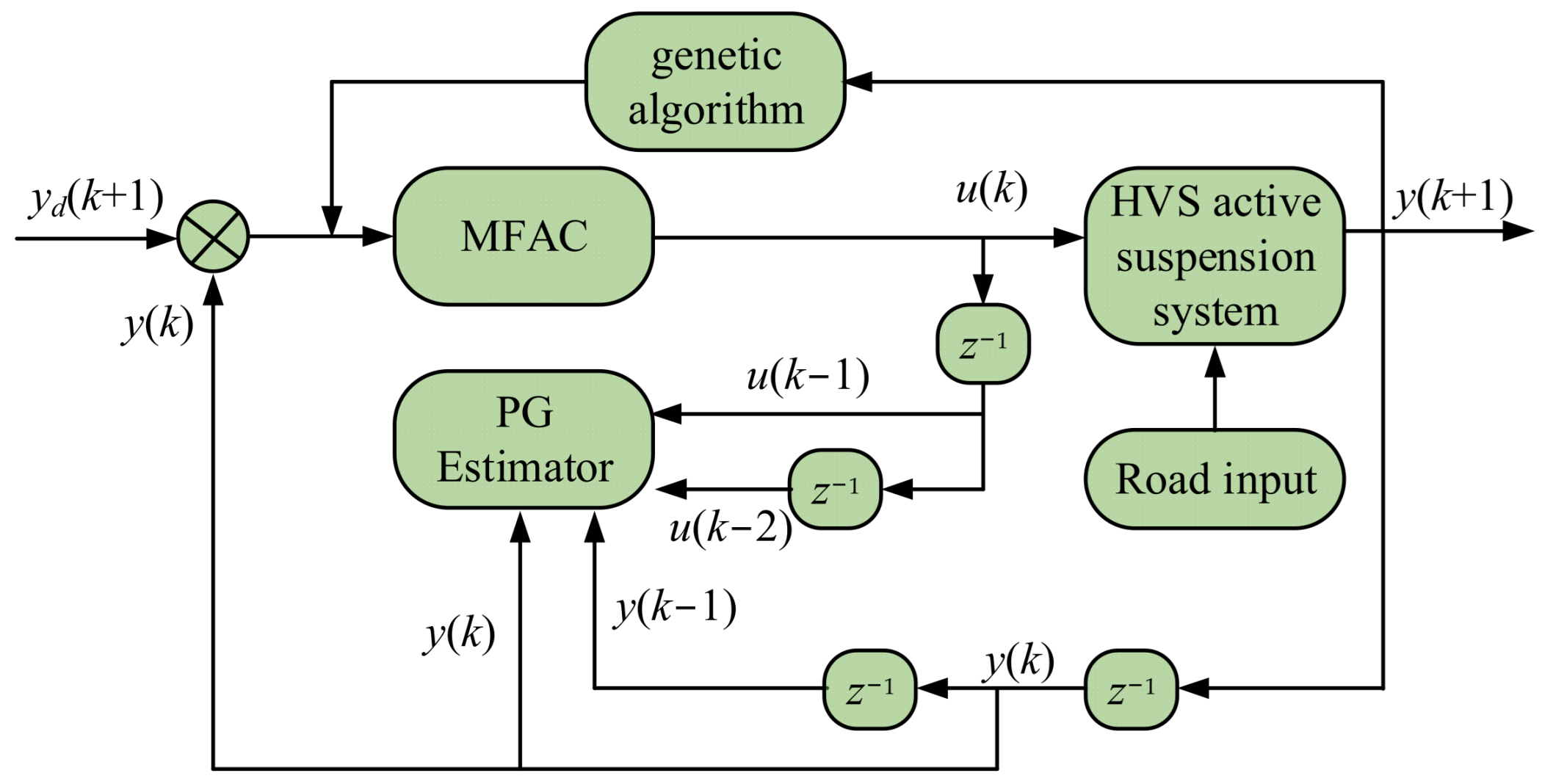
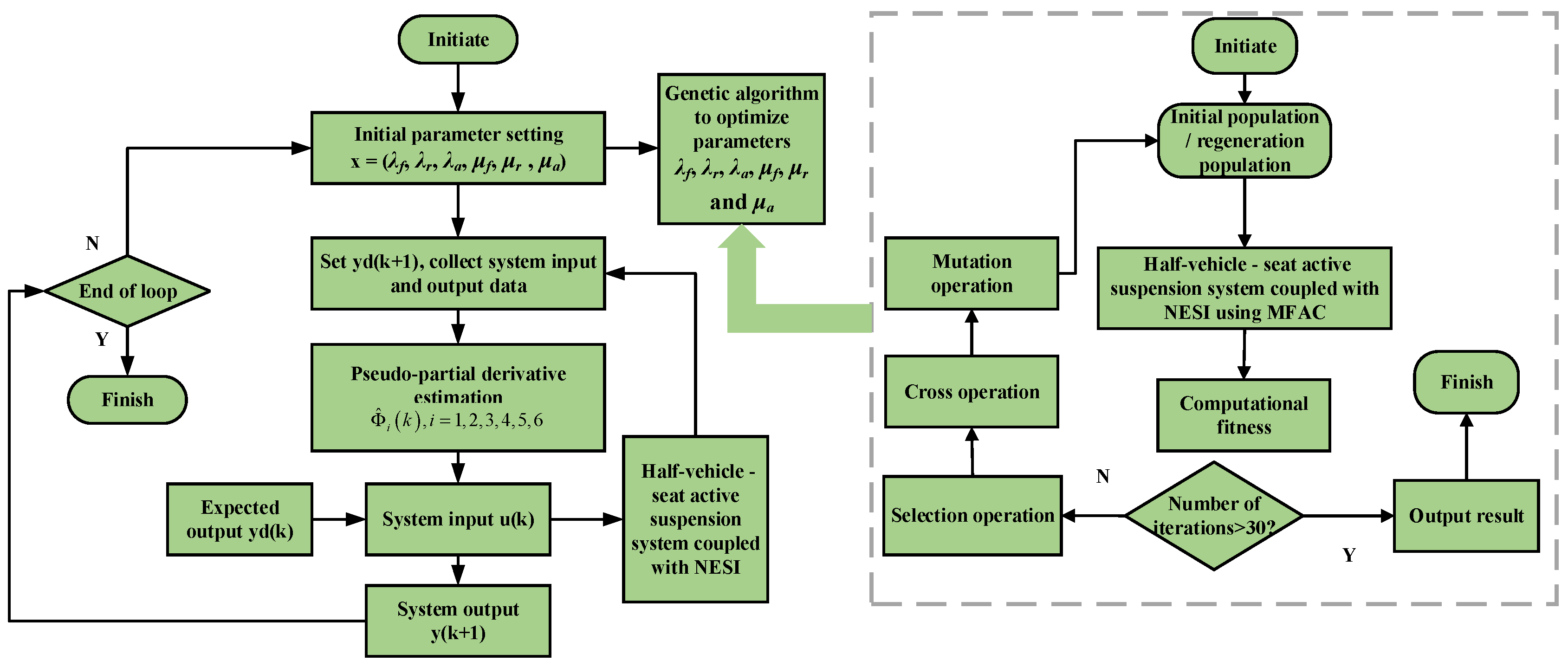
3. MFAC Method Based on Genetic Algorithm

Because the vertical and pitch accelerations of the vehicle body, along with the vertical acceleration of the seat ($z_s^{″}$,${\phi }_s^{″}$,$z_a^{″}$), jointly affect the driver’s ride comfort [36], we define $y={(z_s^{″},{\phi }_s^{″},z_a^{″})}^T$ and $y={(u_f,u_r,u_a)}^T$ as the output and control vectors of the active HVS system coupled with NESI. Taking $y_d={(z_{sd}^{″},{\phi }_{sd}^{″},z_{ad}^{″})}^T={(0,0,0)}^T$ as the control expectation, an MFAC method based on the genetic algorithm is designed and the block diagram is shown in Figure 2.

Figure 2. Block diagram of MFAC method based on genetic algorithm.

Lots of of I/O data are generated when vehicles drive on different pavement surfaces; based on these I/O data, the active HVS system coupled with NESI can be represented as a general discrete-time nonlinear system [37], which is given as

$$y\left(k+1\right)=f\left(y\left(k\right),\cdots y\left(k-n_y\right),u\left(k\right),\cdots u\left(k-n_u\right)\right)$$

(11)

where k is the sampling moment; $u\left(k\right)$ and $y\left(k\right)$ are the inputs and outputs of the system at moment k; $f\left(\cdots \right)={\left[f_1\left(\cdots \right),\cdots ,f_m\left(\cdots \right)\right]}^T\in {\displaystyle \prod _{n_y+n_u+2}{R}^m}\mapsto R^m$ denotes the unknown nonlinear vector function.

$H_{L_{\mathrm{y}},L_{\mathrm{u}}}\left(k\right)={\left[y\left(k\right),\cdots y\left(k-L_y+1\right),u\left(k\right),\cdots u\left(k-L_u+1\right)\right]}^T$ is defined as all input data of time window $\left[k-L_u+1,k\right]$ associated with all output data of time window $\left[k-L_y+1,k\right]$ [38]. The following assumptions are made for a reasonable dynamic linearization of the system.

Assumption 1.

There exist continuous partial derivatives of $f\left(\cdots \right)$ related to $u\left(k\right)$.

Assumption 2.

On the control domain, when $\left|u\left(k\right)\right|\ne 0$, the control system that needs to be dynamically linearized satisfies the generalized Lipschitz continuity condition, which has

$$\left|\Delta y\left(k+1\right)\right|\le a\left|\Delta H_{L_y,L_u}\left(k\right)\right|$$

(12)

where a > 0 is a constant; $\Delta y\left(k\right)=y\left(k\right)-y\left(k-1\right)$; $\Delta H_{L_y,L_u}\left(k\right)=H_{L_y,L_u}\left(k\right)-H_{L_y,L_u}\left(k-1\right)$.

Lemma 1.

For system (11) satisfying Assumptions 1 and 2, when $0\le L_y\le n_y,$ $0\le L_u\le n_u,$ $\Delta H_{L_y,L_u}\left(k\right)\ne 0$, there must exist a pseudo Jacobian matrix $\Phi \left(k\right)$ such that the system (11) can be changed to

$$\Delta y\left(k+1\right)=y\left(k+1\right)-y\left(k\right)={{\Phi }^T}_{f,L_y,L_u}\left(k\right)\Delta H_{L_y,L_u}\left(k\right)$$

(13)

where ${{\Phi }^T}_{f,L_y,L_u}\left(k\right)=\left[{\Phi }_1\left(k\right),\cdots ,{\Phi }_{L_y+L_u}\left(k\right)\right]$ is bounded for any time k.

For ease of calculation, taking $L_y=L_u=3$, we have

$${{\Phi }^T}_{f,L_y,L_u}\left(k\right)=\left[{\Phi }_1\left(k\right),{\Phi }_2\left(k\right),{\Phi }_3\left(k\right),{\Phi }_4\left(k\right),{\Phi }_5\left(k\right),{\Phi }_6\left(k\right)\right]$$

(14)

$$\Delta H_{L_y,L_u}\left(k\right)={\left[\Delta y\left(k\right),\Delta y\left(k-1\right),\Delta u\left(k\right),\Delta u\left(k-1\right)\right]}^T$$

(15)

By bringing Equations (15) and (14) into Equation (13), the dynamical model can be transformed into

$$\begin{array}{l}\Delta y\left(k+1\right)={\Phi }_1\left(k\right)\Delta y\left(k\right)+{\Phi }_2\left(k\right)\Delta y\left(k-1\right)+{\Phi }_3\left(k\right)\Delta y\left(k-2\right)\\ +{\Phi }_4\left(k\right)\Delta u\left(k\right)+{\Phi }_5\left(k\right)\Delta u\left(k-1\right)+{\Phi }_6\left(k\right)\Delta u\left(k-2\right)\end{array}$$

(16)

where ${\Phi }_1\left(k\right),{\Phi }_2\left(k\right),{\Phi }_3\left(k\right),{\Phi }_4\left(k\right),{\Phi }_5\left(k\right),{\Phi }_6\left(k\right)$ is the partial derivative of the system.

To prevent instability in the control system due to excessively large control inputs and the resulting significant errors, the following criterion function for control inputs is introduced:

$$J\left(u\left(k\right)\right)={\left|y_d\left(k+1\right)-y\left(k+1\right)\right|}^2+\lambda {\left|u\left(k\right)-u\left(k-1\right)\right|}^2$$

(17)

where $y_d\left(k+1\right)$ is the desired value; $\lambda$ is a variable coefficient utilized as a weighting factor to constrain variations in the control inputs.

Carrying Equation (16) into Equation (17), deriving derivation for $u\left(k\right)$ and making $u{\left(k\right)}^{\prime }=0$, the MFAC rate can be obtained as follows:

$$\begin{array}{l}u\left(k\right)=u\left(k-1\right)+{\displaystyle \frac{{\rho }_4{\widehat{\Phi }}_4\left(k\right)\left[y^{\ast }\left(k+1\right)-y\left(k\right)\right]}{{\left|{\widehat{\Phi }}_4\left(k\right)\right|}^2+\lambda }}-{\displaystyle \frac{{\widehat{\Phi }}_4\left(k\right){\displaystyle \sum _{i=1}^3{\rho }_i{\Phi }_i}\left(k\right)\Delta u\left(k-i+1\right)}{{\left|{\widehat{\Phi }}_4\left(k\right)\right|}^2+\lambda }}\\ -{\displaystyle \frac{{\widehat{\Phi }}_4\left(k\right){\displaystyle \sum _{i=5}^6{\rho }_i{\Phi }_i}\left(k\right)\Delta u\left(k-3-i+1\right)}{{\left|{\widehat{\Phi }}_4\left(k\right)\right|}^2+\lambda }}\end{array}$$

(18)

where ${\rho }_i\in \left(0,1\right]$ is the step factor, which is introduced to make the MFAC method more flexible, and ${\widehat{\Phi }}_i\left(k\right),i=1,2,3,4,5,6$ is the estimated value of the unknown parameter ${\Phi }_i\left(k\right),i=1,2,3,4,5,6$ with time variation, respectively.

For Equation (18), a critical aspect of designing the control rate is determining the value of the pseudo-partial derivative. However, due to the system’s unknown exact model and the time-varying nature of the pseudo-partial derivative, it is necessary to estimate Φ₁(k), Φ₂(k), Φ₃(k), Φ₄(k), Φ₅(k) and Φ₆(k). Based on the system I/O data for gradient estimation, the following pseudo-partial derivative estimation criterion function is proposed and given by

$$J(\left[\begin{array}{c}{\Phi }_1\left(k\right)\\ {\Phi }_2\left(k\right)\\ {\Phi }_3\left(k\right)\\ {\Phi }_4\left(k\right)\\ {\Phi }_5\left(k\right)\\ {\Phi }_6\left(k\right)\end{array}\right])={\left|\Delta y\left(k\right)-{\left[\begin{array}{c}{\Phi }_1\left(k\right)\\ {\Phi }_2\left(k\right)\\ {\Phi }_3\left(k\right)\\ {\Phi }_4\left(k\right)\\ {\Phi }_5\left(k\right)\\ {\Phi }_6\left(k\right)\end{array}\right]}^T\left[\begin{array}{c}\Delta y\left(k-1\right)\\ \Delta y\left(k-2\right)\\ \Delta y\left(k-3\right)\\ \Delta u\left(k-1\right)\\ \Delta u\left(k-2\right)\\ \Delta u\left(k-3\right)\end{array}\right]\right|}^2+\mu {‖\left[\begin{array}{c}{\Phi }_1\left(k\right)\\ {\Phi }_2\left(k\right)\\ {\Phi }_3\left(k\right)\\ {\Phi }_4\left(k\right)\\ {\Phi }_5\left(k\right)\\ {\Phi }_6\left(k\right)\end{array}\right]-\left[\begin{array}{c}{\widehat{\Phi }}_1\left(k-1\right)\\ {\widehat{\Phi }}_2\left(k-1\right)\\ {\widehat{\Phi }}_3\left(k-1\right)\\ {\widehat{\Phi }}_4\left(k-1\right)\\ {\widehat{\Phi }}_5\left(k-1\right)\\ {\widehat{\Phi }}_6\left(k-1\right)\end{array}\right]‖}^2$$

(19)

The estimation algorithm for Equation (19) can be derived using the matrix inverse lemma for the extrema, resulting in the gradient vector as

$$\left[\begin{array}{c}{\Phi }_1\left(k\right)\\ {\Phi }_2\left(k\right)\\ {\Phi }_3\left(k\right)\\ {\Phi }_4\left(k\right)\\ {\Phi }_5\left(k\right)\\ {\Phi }_6\left(k\right)\end{array}\right]=\left[\begin{array}{c}{\widehat{\Phi }}_1\left(k-1\right)\\ {\widehat{\Phi }}_2\left(k-1\right)\\ {\widehat{\Phi }}_3\left(k-1\right)\\ {\widehat{\Phi }}_4\left(k-1\right)\\ {\widehat{\Phi }}_5\left(k-1\right)\\ {\widehat{\Phi }}_6\left(k-1\right)\end{array}\right]+\eta \left[\begin{array}{c}\Delta y\left(k-1\right)\\ \Delta y\left(k-2\right)\\ \Delta y\left(k-3\right)\\ \Delta u\left(k-1\right)\\ \Delta u\left(k-2\right)\\ \Delta u\left(k-3\right)\end{array}\right]\times {{\displaystyle \frac{\Delta y\left(k\right)-\left[\begin{array}{c}{\widehat{\Phi }}_1\left(k-1\right)\\ {\widehat{\Phi }}_2\left(k-1\right)\\ {\widehat{\Phi }}_3\left(k-1\right)\\ {\widehat{\Phi }}_4\left(k-1\right)\\ {\widehat{\Phi }}_5\left(k-1\right)\\ {\widehat{\Phi }}_6\left(k-1\right)\end{array}\right]\left[\begin{array}{c}\Delta y\left(k-1\right)\\ \Delta y\left(k-2\right)\\ \Delta y\left(k-3\right)\\ \Delta u\left(k-1\right)\\ \Delta u\left(k-2\right)\\ \Delta u\left(k-3\right)\end{array}\right]}{\mu +{\left[\begin{array}{c}\Delta y\left(k-1\right)\\ \Delta y\left(k-2\right)\\ \Delta y\left(k-3\right)\\ \Delta u\left(k-1\right)\\ \Delta u\left(k-2\right)\\ \Delta u\left(k-3\right)\end{array}\right]}^T\left[\begin{array}{c}\Delta y\left(k-1\right)\\ \Delta y\left(k-2\right)\\ \Delta y\left(k-3\right)\\ \Delta u\left(k-1\right)\\ \Delta u\left(k-2\right)\\ \Delta u\left(k-3\right)\end{array}\right]}}}^2$$

(20)

where $\mu >0$ is the weight factor, which directly affects the closed-loop response speed and overshoot of the control system; $\eta \in \left(0,2\right]$ is the step factor and is added to enhance the flexibility of the controller.

To improve the ability of the pseudo-partial derivative estimation algorithm to effectively track time-varying parameters, it is necessary to reset the pseudo-gradient matrix [39]. When $‖{\Phi }_{f,L_y,L_u}\left(k\right)‖\le \epsilon$, $‖\Delta H_{L_y,L_u}\left(k-1\right)‖\le \epsilon$ and $sign\left({\widehat{\Phi }}_4\left(k\right)\right)\ne sign\left({\widehat{\Phi }}_4\left(1\right)\right)$, there is

$${\Phi }_{f,L_y,L_u}\left(k\right)={\Phi }_{f,L_y,L_u}(1)$$

(21)

where ${\Phi }_{f,L_y,L_u}\left(1\right)$ is the original value of ${\Phi }_{f,L_y,L_u}\left(k\right)$; $\epsilon$ is a sufficiently small integer.

Theorem 1.

If the MFAC system satisfies the Assumption 1 and Assumption 2, and there exists a positive constant L and a small positive number $\epsilon$, such that the valuation $\widehat{\Phi }\left(k\right)$ of the pseudo-gradient vector $\Phi \left(k\right)$ for the system meets $\epsilon \le ‖\widehat{\Phi }\left(k\right)‖\le L$, then there is

 (1)

$\left|y\left(k+1\right)-y^{\ast }\left(k+1\right)\right|\le M‖\Delta u\left(k\right)‖$; M is a constant.

 (2)

When $y^{\ast }\left(k+1\right)=y^{\ast }=const$, the parameters ${\mu }_k$ and $\lambda$ choose appropriate values; the system output is bounded and stable.

For the detailed proof of Theorem 1, Hou and Xiong [40] strictly provided a theoretical analysis of the MFAC system based on full-format dynamic linearization, so it is not shown here for brevity.

At present, the value of weight factor λ in Equation (18) and the value of weight factor μ in Equation (20) are usually obtained by the cut-and-try method, and their different values will affect the control effect of the MFAC method. In order to further improve the vibration suppression performance of the active HVS system coupled with NESI, the global optimization genetic algorithm is used to find the best parameter combination in the MFAC method, and the flow chart of the MFAC method based on the genetic algorithm is shown in Figure 3. Since the MFAC method is applied to seat suspension and front and rear suspensions in the active HVS system, the optimization parameters are λ_f, λ_r, λ_a, μ_f, μ_r and μ_a. The upper and lower limits of each variable are shown in Table 2 [41].

Figure 3. Flow chart of MFAC method based on genetic algorithm.

Table 2. Upper and lower values of weight factor for MFAC method.

Variable	Upper Limit	Lower Limit
${\lambda }_f$	0	30
${\lambda }_r$	0	30
${\lambda }_a$	0	30
${\mu }_f$	0	20
${\mu }_r$	0	20
${\mu }_a$	0	20

Based on the author’s previous work, it can be seen that the installation of NESI in the seat suspension and vehicle suspension can significantly reduce the front and rear suspension travel and front and rear dynamic tire loadings, while the seat vertical acceleration and vehicle body vertical and pitch accelerations increase. Therefore, in MFAC design, the weight factor takes zero expected values of seat vertical acceleration and body vertical acceleration and pitch accelerations as the optimization objective and searches for a group of optimal parameter combinations within the parameter ranges of Table 2 to make the controller have the best control effect. Thus, the optimized objective function is

$$f=1/\left({\displaystyle \frac{z_{aa}}{z_{aa0}}}+{\displaystyle \frac{z_{sa}}{z_{sa0}}}+{\displaystyle \frac{{\phi }_a}{z_{a0}}}\right)$$

(22)

where z_aa (z_aa0), z_sa (z_sa0) and φ_a (φ_a0) are the seat vertical acceleration and vehicle body vertical and pitch accelerations of the active and passive HVS systems, respectively. The genetic algorithm is an efficient stochastic search method for solving parameter optimization problems in control engineering, seeking an optimal solution with maximum fitness for the population through selection, crossover, and mutation operations [42].

The six weight factor variables in the optimization model are concatenated from left to right into a coding string x = (λ_f, λ_r, λ_a, μ_f, μ_r, μ_a) and represent one individual in the population. Each individual represents a feasible solution, and the initial population is generated based on the parameters shown in Table 2. The population size is set to 30 and remains constant throughout the iterations. If the selection operation acts on the population with a higher probability, an individual with better fitness is more likely to be selected as a parent for the next generation. The crossover operation occurs with a higher probability and replaces and reorganizes parts of the structure of two parent individuals to generate a new individual. The mutation operation changes parts of an individual with a lower probability to generate a new individual. Following the optimization process shown in Figure 3, the weight factor of the optimized MFAC method is obtained.

4. Random Pavement Excitation

In order to more truly simulate and analyze the dynamic characteristics of the active HVS system under realistic pavement conditions, random pavement excitation is taken as the input excitation on the front and rear wheels. Because the stimulus of pavement roughness is different for different pavement grades and vehicle speeds, we use C-class pavement, a kind of pavement surface that is frequently encountered, which refers to a pavement surface with uneven potholes or large irregularities. Random C-class pavement excitation is often used in the simulation analysis of road roughness. Here, the filtered white noise method is used to simulate the random excitation of C-class pavement, and the dynamic performance of different HVS systems is studied.

The time-domain model of the filtered white noise pavement unevenness is presented as

$$z_r^{\prime }(t)=-2\pi f_0{z}_r(t)+2\pi n_0\sqrt{G_q(n_0)v}\omega (t)$$

(23)

where G_q(n₀) is the pavement unevenness coefficient and set as 64 × 10⁻⁶ m³; v is the vehicle speed; n₀ is the reference spatial frequency and set as 0.011 m⁻¹; f₀ is the time frequency and defined as f₀ = n₀ × v₀; ω(t) is Gaussian white noise with a unit intensity of 1. The rear tire pavement input excitation has a time lag relative to the front tire pavement input excitation, as described by Equation (24), and the random excitation is illustrated in Figure 4.

$$z_{rr}(t)=z_{rf}(t-\tau )$$

(24)

Figure 4. Pavement random excitation of the front and rear tires.

The structural parameters of the active HVS system are listed in Table 1. The controller parameters of the MFAC method are η = 2, ρ₁ = 0.4, ρ₂ = 0.1, ρ₃ = 0.7, ρ₄ = 0.7, ρ₅ = 0.2, ρ₆ = 0.5, Φ_1c = 0.03, Φ_2c = 0.03, Φ_3c = 0.03, Φ_4c = 0.03, Φ_5c = 0.03, and Φ_6c = 0.03. The optimized weight factors of the MFAC method are obtained as λ_f = 21.31151, λ_r = 25.5732, λ_a = 11.2246, u_f = 6.2475, u_r = 9.3943, and u_a = 11.5437. The dynamic performances of the original HVS system, HVS system coupled with NESI, and active HVS system coupled with NESI using the PID and MFAC methods are compared to demonstrate the benefit of NESI and illustrate the effectiveness of the MFAC method.

The dynamic equations of the original HVS system are given as

$$\left\{\begin{array}{l}{m}_s{z}_s^{″}+(c_r{l}_r-c_f{l}_f-c_a{l}_a){\phi }^{\prime }+(c_f+c_r+c_a)z_s^{\prime }+(k_r{l}_r-k_f{l}_f-k_a{l}_a)\phi \\ -c_f{z}_{uf}^{\prime }-c_r{z}_{ur}^{\prime }-c_a{z}_a^{\prime }+(k_f+k_r+k_a)z_s-k_f{z}_{uf}-k_r{z}_{ur}+k_a(z_s-l_a\phi -z_a)=0\\ \\ I_{\phi }{\phi }^{″}+(c_r{l}_r^2+c_f{l}_f^2+c_a{l}_a^2){\phi }^{\prime }+(c_r{l}_r-c_f{l}_f-c_a{l}_a)z_s^{\prime }+(k_r{l}_r^2+k_f{l}_f^2)\phi \\ +c_f{l}_f{z}_{uf}^{\prime }-c_r{l}_r{z}_{ur}^{\prime }+c_a{l}_a{z}_a^{\prime }+(k_r{l}_r-k_f{l}_f)z_s+k_f{l}_f{z}_{uf}-k_r{l}_r{z}_{ur}\\ -k_a{l}_a(z_s-l_a\phi -z_a)=0\\ \\ c_f{l}_f{\phi }^{\prime }+m_{uf}{z}_{uf}^{″}-c_f{z}_s^{\prime }+k_f{l}_f\phi +c_f{z}_{uf}^{\prime }-k_f{z}_s+(k_f+k_{tf})z_{uf}=k_{tf}{z}_{rf}\\ \\ m_{ur}{z}_{ur}^{″}-c_r{l}_r{\phi }^{\prime }-c_r{z}_s^{\prime }-k_r{l}_r\phi +c_r{z}_{ur}^{\prime }-k_r{z}_s+(k_r+k_{tr})z_{ur}=k_{tr}{z}_{rr}\\ \\ c_a{l}_a{\phi }^{\prime }+m_a{z}_a^{″}-c_a{z}_s^{\prime }+c_a{z}_a^{\prime }+k_a(z_a-z_s+l_a\phi )=0\end{array}\right.$$

(25)

The dynamic equations of the HVS system coupled with NESI are presented as

$$\left\{\begin{array}{l}{m}_s{z}_s^{″}-b_a(z_{ba}^{″}-z_{sa}^{″})+c_f(z_{sf}^{\prime }-z_{uf}^{\prime })+c_r(z_{sr}^{\prime }-z_{ur}^{\prime })+c_a(z_{sa}^{\prime }-z_a^{\prime })+k_f(z_{sf}-z_{uf})\\ +k_r(z_{sr}-z_{ur})+k_a(z_{sa}-z_a)+c_{bf}(z_{sf}^{\prime }-z_{bf}^{\prime })+c_{br}(z_{sr}^{\prime }-z_{br}^{\prime })+k_{bf}(z_{sf}-z_{bf}{)}^3\\ +k_{br}(z_{sr}-z_{br}{)}^3=0\\ \\ I_{\phi }{\phi }^{″}+c_r{l}_r(z_{sr}^{\prime }-z_{ur}^{\prime })-c_f{l}_f(z_{sf}^{\prime }-z_{uf}^{\prime })-c_a{l}_a(z_{sa}^{\prime }-z_a^{\prime })+k_r{l}_r(z_{sr}-z_{ur})-\\ k_f{l}_f(z_{sf}-z_{uf})-k_a{l}_a(z_{sa}-z_a)+b_a(z_{ba}^{″}-z_{sa}^{″})l_a+c_{br}{l}_r(z_{sr}^{\prime }-z_{br}^{\prime })\\ -c_{bf}{l}_f(z_{sf}^{\prime }-z_{bf}^{\prime })+k_{br}{l}_r(z_{sr}-z_{br}{)}^3-k_{bf}{l}_f(z_{sf}-z_{bf}{)}^3=0\\ \\ (m_{uf}+b_f)z_{uf}^{″}-b_f{z}_{bf}^{″}-c_f{z}_{sf}^{\prime }+c_f{z}_{uf}^{\prime }-k_f{z}_{sf}+(k_f+k_{tf})z_{uf}=k_{tf}{z}_{rf}\\ \\ (m_{ur}+b_r)z_{ur}^{″}-b_r{z}_{br}^{″}-c_r{z}_{sr}^{\prime }+c_r{z}_{ur}^{\prime }-k_r{z}_{sr}+(k_r+k_{tr})z_{ur}=k_{tr}{z}_{rr}\\ \\ m_a{z}_a^{″}+c_a(z_a^{\prime }-z_{sa}^{\prime })+k_a(z_a-z_{sa})+k_{ba}(z_a-z_{ba}{)}^3+c_{ba}(z_a^{\prime }-z_{ba}^{\prime })=0\\ \\ b_a(z_{ba}^{″}-z_{sa}^{″})-k_{ba}(z_a-z_{ba}{)}^3-c_{ba}(z_a^{\prime }-z_{ba}^{\prime })=0\\ \\ b_f{z}_{bf}^{″}-b_f{z}_{uf}^{″}-c_{bf}{z}_{sf}^{\prime }+c_{bf}{z}_{bf}^{\prime }+k_{bf}(z_{bf}-z_{sf}{)}^3=0\\ \\ b_r{z}_{br}^{″}-b_r{z}_{ur}^{″}-c_{br}{z}_{sr}^{\prime }+c_{br}{z}_{br}^{\prime }+k_{br}(z_{br}-z_{sr}{)}^3=0\end{array}\right.$$

(26)

The dynamic equations of the active HVS system coupled with NESI using the PID control method are similar to Equation (10); the PID control algorithm formula is given as

$$u\left(t\right)=k_p\cdot e\left(t\right)+k_i\cdot {\displaystyle \int e\left(t\right)}dt+k_d\cdot {\displaystyle \frac{de\left(t\right)}{dt}}$$

(27)

where u(t) is the output of the PID controller and $u\left(t\right)={(u_f,u_r,u_a)}^T$; e(t) is the deviation of the system (the difference between the expected value $y_d={(z_{sd}^{″},{\phi }_{sd}^{″},z_{ad}^{″})}^T$ and the actual value $y={(z_s^{″},{\phi }_s^{″},z_a^{″})}^T$); k_p, k_i and k_d are the proportional, integral, and differential coefficients. The PID controller parameters applied in the seat suspension using the genetic algorithm are determined as k_pa = 87.8986, k_ia = 67.017, and k_da = 1.3419; the PID controller parameters applied in the front and rear suspensions using the genetic algorithm are determined as k_pf = 90.3278, k_if = 92.1107, k_df = 1.7559, k_pr = 79.5577, k_ir = 99.7640, and k_dr = 9.9472.

The dynamic performance of these HVS systems is evaluated using seven evaluation indicators, including seat vertical acceleration, vehicle body vertical and pitch accelerations (z_aa, z_sa, φ_a), front suspension travel (z_sf–z_uf, J_sssf), rear suspension travel (z_sr–z_ur, J_sssr), front dynamic tire loading (k_tf(z_uf–z_rf), J_DTLf), and rear dynamic tire loading (k_tr(z_ur–z_rr), J_DTLr), respectively. Figure 5 shows the dynamic performance evaluation indicators of different HVS systems under random pavement excitation at a vehicle speed of 15 m/s. To more clearly observe the dynamic performance of each HVS system at different vehicle speeds, Table 3 provides the root mean square (RMS) values of the seven evaluation indicators for the four HVS systems at vehicle speeds of 5, 10, 15, 20, 25 and 30 m/s, with the corresponding line graphs shown in Figure 6. It can be seen from Figure 5 and Figure 6 that the RMS(z_sa), RMS(φ_a), RMS(z_aa), RMS(J_sssf), RMS(J_sssr), RMS(J_DTLf) and RMS(J_DTLr) for the HVS system coupled with NESIs are all lower than those of the original HVS system at different vehicle speeds, which shows the advantage of NESI. Figure 6a–e show that the RMS(z_sa), RMS(φ_a), RMS(z_aa), RMS(J_sssf) and RMS(J_sssr) for the active HVS system coupled with NESI using the MFAC method are significantly smaller than those of the original HVS system, the HVS system coupled with NESI, and the active HVS system coupled with NESI using the PID control method; Figure 6f,g show that the RMS(J_DTLf) and RMS(J_DTLr) are also slightly smaller than those of the other three HVS systems, which reflects the best dynamic performance among the four HVS systems and shows the effectiveness of the MFAC method.

Figure 5. Dynamic performance evaluation indicators of different HVS systems under random pavement excitation (v = 15 m/s).

Table 3. RMS values of dynamic performance evaluation indicators for different HVS systems under random pavement excitation at different vehicle speeds.

Speed	Indicators	Original	NESI	PID	MFAC
5 m/s	RMS(zsa)	0.2668 m/s2	0.2531 m/s2	0.2157 m/s2	0.1424 m/s2
	RMS(${\phi }_a$)	0.2464 rad/s2	0.2099 rad/s2	0.1711 rad/s2	0.1261 rad/s2
	RMS(zaa)	0.2977 m/s2	0.2174 m/s2	0.1252 m/s2	0.0629 m/s2
	RMS(Jsssf)	0.0051 m	0.0047 m	0.0047 m	0.0035 m
	RMS(Jsssr)	0.0048 m	0.0043 m	0.0042 m	0.0037 m
	RMS(JDTLf)	320.0783 N	265.4598 N	263.0662 N	253.0396 N
	RMS(JDTLr)	331.3083 N	274.6861 N	271.1194 N	259.0869 N
10 m/s	RMS(zsa)	0.4284 m/s2	0.3658 m/s2	0.3056 m/s2	0.1925 m/s2
	RMS(${\phi }_a$)	0.3246 rad/s2	0.2951 rad/s2	0.2512 rad/s2	0.1831 rad/s2
	RMS(zaa)	0.3844 m/s2	0.2982 m/s2	0.1732 m/s2	0.0909 m/s2
	RMS(Jsssf)	0.0071 m	0.0067 m	0.0065 m	0.0053 m
	RMS(Jsssr)	0.0071 m	0.0058 m	0.0053 m	0.0044 m
	RMS(JDTLf)	452.0866 N	378.6121 N	373.8854 N	354.6754 N
	RMS(JDTLr)	472.6359 N	387.9935 N	386.5476 N	361.2199 N
15 m/s	RMS(zsa)	0.5600 m/s2	0.4765 m/s2	0.3831 m/s2	0.2425 m/s2
	RMS(${\phi }_a$)	0.3702 rad/s2	0.3411 rad/s2	0.2956 rad/s2	0.2187 rad/s2
	RMS(zaa)	0.4603 m/s2	0.3588 m/s2	0.2137 m/s2	0.1071 m/s2
	RMS(Jsssf)	0.0088 m	0.0083 m	0.0080 m	0.0069 m
	RMS(Jsssr)	0.0087 m	0.0072 m	0.0069 m	0.0053 m
	RMS(JDTLf)	554.0991 N	465.7717 N	460.4525 N	435.7612 N
	RMS(JDTLr)	552.5659 N	478.8739 N	475.7574 N	441.6093 N
20 m/s	RMS(zsa)	0.6332 m/s2	0.5498 m/s2	0.4515 m/s2	0.2796 m/s2
	RMS(${\phi }_a$)	0.4368 rad/s2	0.3926 rad/s2	0.3345 rad/s2	0.2484 rad/s2
	RMS(zaa)	0.5278 m/s2	0.4105 m/s2	0.2341 m/s2	0.1245 m/s2
	RMS(Jsssf)	0.0102 m	0.0095 m	0.0094 m	0.0077 m
	RMS(Jsssr)	0.0100 m	0.0083 m	0.0081 m	0.0059 m
	RMS(JDTLf)	639.6182 N	534.7238 N	526.4452 N	505.9133 N
	RMS(JDTLr)	669.1567 N	544.4752 N	541.7558 N	504.0269 N
25 m/s	RMS(zsa)	0.7112 m/s2	0.6236 m/s2	0.5219 m/s2	0.3126 m/s2
	RMS(${\phi }_a$)	0.4798 rad/s2	0.4285 rad/s2	0.3617 rad/s2	0.2851 rad/s2
	RMS(zaa)	0.5814 m/s2	0.4542 m/s2	0.2535 m/s2	0.1421 m/s2
	RMS(Jsssf)	0.0113 m	0.0105 m	0.0103 m	0.0094 m
	RMS(Jsssr)	0.0110 m	0.0093 m	0.0092 m	0.0068 m
	RMS(JDTLf)	708.4648 N	598.0734 N	585.2245 N	573.9021 N
	RMS(JDTLr)	721.6675 N	608.4276 N	608.3457 N	571.1349 N
30 m/s	RMS(zsa)	0.8282 m/s2	0.6911 m/s2	0.5945 m/s2	0.3504 m/s2
	RMS(${\phi }_a$)	0.4702 rad/s2	0.4592 rad/s2	0.4156 rad/s2	0.3122 rad/s2
	RMS(zaa)	0.6341 m/s2	0.4925 m/s2	0.2841 m/s2	0.1584 m/s2
	RMS(Jsssf)	0.0123 m	0.0113 m	0.0110 m	0.0095 m
	RMS(Jsssr)	0.0120 m	0.0101 m	0.0099 m	0.0081 m
	RMS(JDTLf)	781.7247 N	655.6325 N	650.1521 N	631.9343 N
	RMS(JDTLr)	780.9716 N	683.0428 N	675.1251 N	654.8734 N

Figure 6. Line graphs of RMS values of dynamic performance evaluation indicators for different HVS systems under random pavement excitation at different vehicle speeds.

Building on the above analysis, the influence of the installed position of MFAC on the dynamic performance of the active HVS system coupled with NESI is further examined, where one MFAC acting on the seat suspension and two MFACs acting on the front and rear suspensions are evaluated. When the MFAC is acting only on the seat suspension, the corresponding dynamic equations are

$$\left\{\begin{array}{l}{m}_s{z}_s^{″}-b_a(z_{ba}^{″}-z_{sa}^{″})+c_f(z_{sf}^{\prime }-z_{uf}^{\prime })+c_r(z_{sr}^{\prime }-z_{ur}^{\prime })+c_a(z_{sa}^{\prime }-z_a^{\prime })+k_f(z_{sf}-z_{uf})\\ +k_r(z_{sr}-z_{ur})+k_a(z_{sa}-z_a)+c_{bf}(z_{sf}^{\prime }-z_{bf}^{\prime })+c_{br}(z_{sr}^{\prime }-z_{br}^{\prime })+k_{bf}(z_{sf}-z_{bf}{)}^3\\ +k_{br}(z_{sr}-z_{br}{)}^3-u_a=0\\ \\ I_{\phi }{\phi }^{″}+c_r{l}_r(z_{sr}^{\prime }-z_{er}^{\prime })-c_f{l}_f(z_{sf}^{\prime }-z_{uf}^{\prime })-c_a{l}_a(z_{sa}^{\prime }-z_a^{\prime })+k_r{l}_r(z_{sr}-z_{ur})\\ -k_f{l}_f(z_{sf}-z_{uf})-k_a{l}_a(z_{sa}-z_a)+b_a(z_{ba}^{″}-z_{sa}^{″})l_a+c_{br}{l}_r(z_{sr}^{\prime }-z_{br}^{\prime })\\ -c_{bf}{l}_f(z_{sf}^{\prime }-z_{bf}^{\prime })+k_{br}{l}_r(z_{sr}-z_{br}{)}^3-k_{bf}{l}_f(z_{sf}-z_{bf}{)}^3+l_a{u}_a=0\\ \\ (m_{uf}+b_f)z_{uf}^{″}-b_f{z}_{bf}^{″}-c_f{z}_{sf}^{\prime }+c_f{z}_{sf}^{\prime }-k_f{z}_{sf}+(k_f+k_{tf})z_{uf}=k_{tf}{z}_{rf}\\ \\ (m_{ur}+b_r)z_{ur}^{″}-b_r{z}_{br}^{″}-c_r{z}_{sr}^{\prime }+c_r{z}_{ur}^{\prime }-k_r{z}_{sr}+(k_r+k_{tr})z_{ur}=k_{tr}{z}_{rr}\\ \\ m_a{z}_a^{″}+c_a(z_a^{\prime }-z_{sa}^{\prime })+k_a(z_a-z_{sa})+k_{ba}(z_a-z_{ba}{)}^3+c_{ba}(z_a^{\prime }-z_{ba}^{\prime })-u_a=0\\ \\ b_a(z_{ba}^{″}-z_{sa}^{″})-k_{ba}(z_a-z_{ba}{)}^3-c_{ba}(z_a^{\prime }-z_{ba}^{\prime })=0\\ \\ b_f{z}_{bf}^{″}-b_f{z}_{uf}^{″}-c_{bf}{z}_{sf}^{\prime }+c_{bf}{z}_{bf}^{\prime }+k_{bf}(z_{bf}-z_{sf}{)}^3=0\\ \\ b_r{z}_{br}^{″}-b_r{z}_{ur}^{″}-c_{br}{z}_{sr}^{\prime }+c_{br}{z}_{br}^{\prime }+k_{br}(z_{br}-z_{sr}{)}^3=0\end{array}\right.$$

(28)

When the MFAC is acting on the front and rear suspensions, the corresponding dynamic equations are

$$\left\{\begin{array}{l}{m}_s{z}_s^{″}-b_a(z_{ba}^{″}-z_{sa}^{″})+c_f(z_{sf}^{\prime }-z_{uf}^{\prime })+c_r(z_{sr}^{\prime }-z_{ur}^{\prime })+c_a(z_{sa}^{\prime }-z_a^{\prime })+k_f(z_{sf}-z_{uf})\\ +k_r(z_{sr}-z_{ur})+k_a(z_{sa}-z_a)+c_{bf}(z_{sf}^{\prime }-z_{bf}^{\prime })+c_{br}(z_{sr}^{\prime }-z_{br}^{\prime })+k_{bf}(z_{sf}-z_{bf}{)}^3\\ +k_{br}(z_{sr}-z_{br}{)}^3-u_f-u_r=0\\ \\ I_{\phi }{\phi }^{″}+c_r{l}_r(z_{sr}^{\prime }-z_{ur}^{\prime })-c_f{l}_f(z_{sf}^{\prime }-z_{uf}^{\prime })-c_a{l}_a(z_{sa}^{\prime }-z_a^{\prime })+k_r{l}_r(z_{sr}-z_{ur})\\ -k_f{l}_f(z_{sf}-z_{uf})-k_a{l}_a(z_{sa}-z_a)+b_a(z_{ba}^{″}-z_{sa}^{″})l_a+c_{br}{l}_r(z_{sr}^{\prime }-z_{br}^{\prime })\\ -c_{bf}{l}_f(z_{sf}^{\prime }-z_{bf}^{\prime })+k_{br}{l}_r(z_{sr}-z_{br}{)}^3-k_{bf}{l}_f(z_{sf}-z_{bf}{)}^3+l_f{u}_f-l_r{u}_r=0\\ \\ (m_{uf}+b_f)z_{uf}^{″}-b_f{z}_{bf}^{″}-c_f{z}_{sf}^{\prime }+c_f{z}_{uf}^{\prime }-k_f{z}_{sf}+(k_f+k_{tf})z_{uf}-u_f=k_{tf}{z}_{rf}\\ \\ (m_{ur}+b_r)z_{ur}^{″}-b_r{z}_{br}^{″}-c_r{z}_{sr}^{\prime }+c_r{z}_{ur}^{\prime }-k_r{z}_{sr}+(k_r+k_{tr})z_{ur}-u_r=k_{tr}{z}_{rr}\\ \\ m_a{z}_a^{″}+c_a(z_a^{\prime }-z_{sa}^{\prime })+k_a(z_a-z_{sa})+k_{ba}(z_a-z_{ba}{)}^3+c_{ba}(z_a^{\prime }-z_{ba}^{\prime })=0\\ \\ b_a(z_{ba}^{″}-z_{sa}^{″})-k_{ba}(z_a-z_{ba}{)}^3-c_{ba}(z_a^{\prime }-z_{ba}^{\prime })=0\\ \\ b_f{z}_{bf}^{″}-b_f{z}_{uf}^{″}-c_{bf}{z}_{sf}^{\prime }+c_{bf}{z}_{bf}^{\prime }+k_{bf}(z_{bf}-z_{sf}{)}^3=0\\ \\ b_r{z}_{br}^{″}-b_r{z}_{ur}^{″}-c_{br}{z}_{sr}^{\prime }+c_{br}{z}_{br}^{\prime }+k_{br}(z_{br}-z_{sr}{)}^3=0\end{array}\right.$$

(29)

Figure 7 shows the dynamic performance evaluation indicators of three active and passive HVS systems under pavement random excitation with vehicle speed chosen as 15 m/s; the detailed RMS values of the seven evaluation indicators at different vehicle speeds are displayed in Table 4, and the corresponding line graphs are shown in Figure 8. The terms MFAC1, MFAC2 and MFAC3 refer to the MFAC acting on the seat suspension, MFAC acting on the front and rear suspensions, and MFAC acting on the seat and vehicle suspensions for the active HVS system coupled with NESI. Figure 8d–g show that when the MFAC is acting on the seat and vehicle suspensions, the RMS(J_sssf), RMS(J_sssr), RMS(J_DTLf) and RMS(J_DTLr) are smaller than those of the other three HVS systems; the RMS(z_aa) is smaller than those of the passive HVS system and active HVS system where the MFAC is acting on the front and rear suspensions, while it is larger than that of the active HVS system where the MFAC is acting on the seat suspension; Figure 8a,b show that the RMS(z_sa) and RMS(φ_a) are smaller than those of the passive HVS system and active HVS system where the MFAC is acting on the seat suspension, while it is larger than that of the active HVS system where the MFAC is acting on the front and rear suspensions. Thus, when the MFAC is acting on the seat and vehicle suspensions, the active HVS system achieves the best dynamic performance.

Figure 7. Dynamic performance evaluation indicators of three active and passive HVS systems under random pavement excitation (v = 15 m/s).

Table 4. RMS values of dynamic performance evaluation indicators for three active and passive HVS systems under random pavement excitation at different vehicle speeds.

Speed	Indicators	Passive	MFAC1	MFAC2	MFAC3
5 m/s	RMS(zsa)	0.2531 m/s2	0.2182 m/s2	0.1342 m/s2	0.1424 m/s2
	RMS(${\phi }_a$)	0.2099 rad/s2	0.1718 rad/s2	0.1105 rad/s2	0.1261 rad/s2
	RMS(zaa)	0.2174 m/s2	0.0609 m/s2	0.1047 m/s2	0.0629 m/s2
	RMS(Jsssf)	0.0047 m	0.0039 m	0.0036 m	0.0035 m
	RMS(Jsssr)	0.0043 m	0.0040 m	0.0037 m	0.0037 m
	RMS(JDTLf)	265.4598 N	265.3441 N	260.3031 N	253.0396 N
	RMS(JDTLr)	274.6861 N	271.1274 N	269.7326 N	259.0869 N
10 m/s	RMS(zsa)	0.3658 m/s2	0.2962 m/s2	0.1678 m/s2	0.1925 m/s2
	RMS(${\phi }_a$)	0.2951 rad/s2	0.2560 rad/s2	0.1531 rad/s2	0.1597 rad/s2
	RMS(zaa)	0.2982 m/s2	0.0837 m/s2	0. 1184 m/s2	0.0909 m/s2
	RMS(Jsssf)	0.0067 m	0.0057 m	0.0054 m	0.0053 m
	RMS(Jsssr)	0.0058 m	0.0058 m	0.0045 m	0.0044 m
	RMS(JDTLf)	378.6121 N	374.6261 N	361.5634 N	354.6754 N
	RMS(JDTLr)	387.9935 N	380.8379 N	371.0558 N	361.2199 N
15 m/s	RMS(zsa)	0.4765 m/s2	0.3881 m/s2	0.2125 m/s2	0.2425 m/s2
	RMS(${\phi }_a$)	0.3411 rad/s2	0.2988 rad/s2	0.1915 rad/s2	0.2187 rad/s2
	RMS(zaa)	0.3588 m/s2	0.1027 m/s2	0.1244 m/s2	0.1071 m/s2
	RMS(Jsssf)	0.0083 m	0.0078 m	0.0076 m	0.0069 m
	RMS(Jsssr)	0.0072 m	0.0065 m	0.0059 m	0.0053 m
	RMS(JDTLf)	465.7717 N	458.5251 N	456.0713 N	435.7612 N
	RMS(JDTLr)	478.8739 N	472.7714 N	451.0862 N	441.6093 N
20 m/s	RMS(zsa)	0.5498 m/s2	0.4450 m/s2	0.2413 m/s2	0.2796 m/s2
	RMS(${\phi }_a$)	0.3926 rad/s2	0.3469 rad/s2	0.2156 rad/s2	0.2484 rad/s2
	RMS(zaa)	0.4105 m/s2	0.1139 m/s2	0.1454 m/s2	0.1245 m/s2
	RMS(Jsssf)	0.0095 m	0.0086 m	0.0080 m	0.0077 m
	RMS(Jsssr)	0.0083 m	0.0078 m	0.0063 m	0.0059 m
	RMS(JDTLf)	534.7238 N	528.9467 N	520.3906 N	505.9133 N
	RMS(JDTLr)	544.4752 N	538.6432 N	520.6340 N	504.0269 N
25 m/s	RMS(zsa)	0.6236 m/s2	0.5110 m/s2	0.2732 m/s2	0.3126 m/s2
	RMS(${\phi }_a$)	0.4285 rad/s2	0.3752 rad/s2	0.2524 rad/s2	0.2851 rad/s2
	RMS(zaa)	0.4542 m/s2	0.1216 m/s2	0.1641 m/s2	0.1421 m/s2
	RMS(Jsssf)	0.0105 m	0.0099 m	0.0095 m	0.0094 m
	RMS(Jsssr)	0.0093 m	0.0089 m	0.0085 m	0.0068 m
	RMS(JDTLf)	598.0734 N	590.9013 N	582.9449 N	573.9021 N
	RMS(JDTLr)	608.4276 N	604.3024 N	591.6629 N	571.1349 N
30 m/s	RMS(zsa)	0.6911 m/s2	0.5857 m/s2	0.3192 m/s2	0.3504 m/s2
	RMS(${\phi }_a$)	0.4592 rad/s2	0.3862 rad/s2	0.2703 rad/s2	0.3122 rad/s2
	RMS(zaa)	0.4925 m/s2	0.1372 m/s2	0.1823 m/s2	0.1584 m/s2
	RMS(Jsssf)	0.0113 m	0.0109 m	0.0102 m	0.0095 m
	RMS(Jsssr)	0.0101 m	0.0098 m	0.0086 m	0.0081 m
	RMS(JDTLf)	655.6325 N	646.6703 N	635.3834 N	631.9343 N
	RMS(JDTLr)	683.0428 N	680.5100 N	678.4872 N	654.8734 N

Figure 8. Line graphs of RMS values of dynamic performance evaluation indicators for three active and passive HVS systems under random pavement excitation at different vehicle speeds.

5. Pavement Shock Excitation

Considering the pavement shock excitation caused by discrete irregularities (such as bumps or potholes), the shock excitation applied in the front and rear tires is denoted as

$$\begin{array}{l}{z}_{rf}=\left\{\begin{array}{c}{\displaystyle \frac{A_b}{2}}\left[1-\cos \left({\displaystyle \frac{2\pi v}{L}}t\right)\right]\\ 0\end{array}\right.\begin{array}{c}0\le t<{\displaystyle \frac{L}{v}}\\ t\ge {\displaystyle \frac{L}{v}}\end{array}\\ z_{rf}=\left\{\begin{array}{c}0\\ {\displaystyle \frac{A_b}{2}}\left[1-\cos \left({\displaystyle \frac{2\pi v}{L}}(t-{\displaystyle \frac{l_f+l_r}{v}})\right)\right]\\ 0\end{array}\begin{array}{c}0\le t<{\displaystyle \frac{L}{v}}\\ {\displaystyle \frac{l_f+l_r}{v}}\le t<{\displaystyle \frac{l_f+l_r+L}{v}}\\ t\ge {\displaystyle \frac{l_f+l_r+L}{v}}\end{array}\right.\end{array}$$

(30)

where $A_b(A_b=0.1 \mathrm{m})$ and $L(L=2 \mathrm{m})$ are the height and length of the pavement bulge, respectively. $(l_f+l_r)/v$ is the rear tire time delay; the pavement shock excitation is illustrated in Figure 9.

Figure 9. Pavement shock excitation.

Figure 10 shows the dynamic performance evaluation indicators of different HVS systems under pavement shock excitation, considering that the common vehicle speed under pavement shock excitation is between 15 km/h and 35 km/h; the vehicle speed is chosen as 5 m/s here. Figure 10a–e show that, compared with the other three HVS systems, the peak amplitudes of z_sa, φ_a, z_aa, J_sssf and J_sssr of the active HVS system coupled with NESI using the MFAC method reduce and the vibration attenuation time shortens; Figure 10f,g show that, compared with the other three HVS systems, the peak amplitudes of J_DTLf and J_DTLr of the active HVS system coupled with NESI using the MFAC method increase, while the vibration attenuation time decreases.

Figure 10. Dynamic performance evaluation indicators of different HVS systems under pavement shock excitation (v = 5 m/s).

Figure 11 shows the dynamic performance evaluation indicators of three active and passive HVS systems under random pavement excitation with the vehicle speed chosen as 5 m/s. Figure 11a–e show when the MFAC is acting on the seat and vehicle suspensions, the peak amplitudes and vibration attenuation time of z_sa, φ_a, z_aa, J_sssf and J_sssr are slightly smaller than those of the active HVS system where the MFAC is acting on the front and rear suspensions, and are significantly smaller than those of the passive HVS system and active HVS system where the MFAC is acting on the seat suspension; Figure 11f,g show that when the MFAC is acting on the seat and vehicle suspensions, the peak amplitudes of J_DTLf and J_DTLr are larger than those of the passive and other two active HVS systems, while the vibration attenuation time decreases slightly.

Figure 11. Dynamic performance evaluation indicators of three active and passive HVS systems under pavement shock excitation (v = 5 m/s).

6. Conclusions

In this paper, the NESI is applied in the seat suspension and vehicle suspension for the HVS system, and the MFAC method based on the genetic algorithm is designed to further enhance the dynamic performance. The dynamic model of the active HVS system coupled with NESI using the MFAC method is established; its dynamic response under pavement random and shock excitations are acquired, and the dynamic performance is evaluated. The effectiveness of the MFAC method is revealed and the influence of the installed position of MFAC on the dynamic performance of the HVS system is studied. The main conclusions are as follows:

(1)

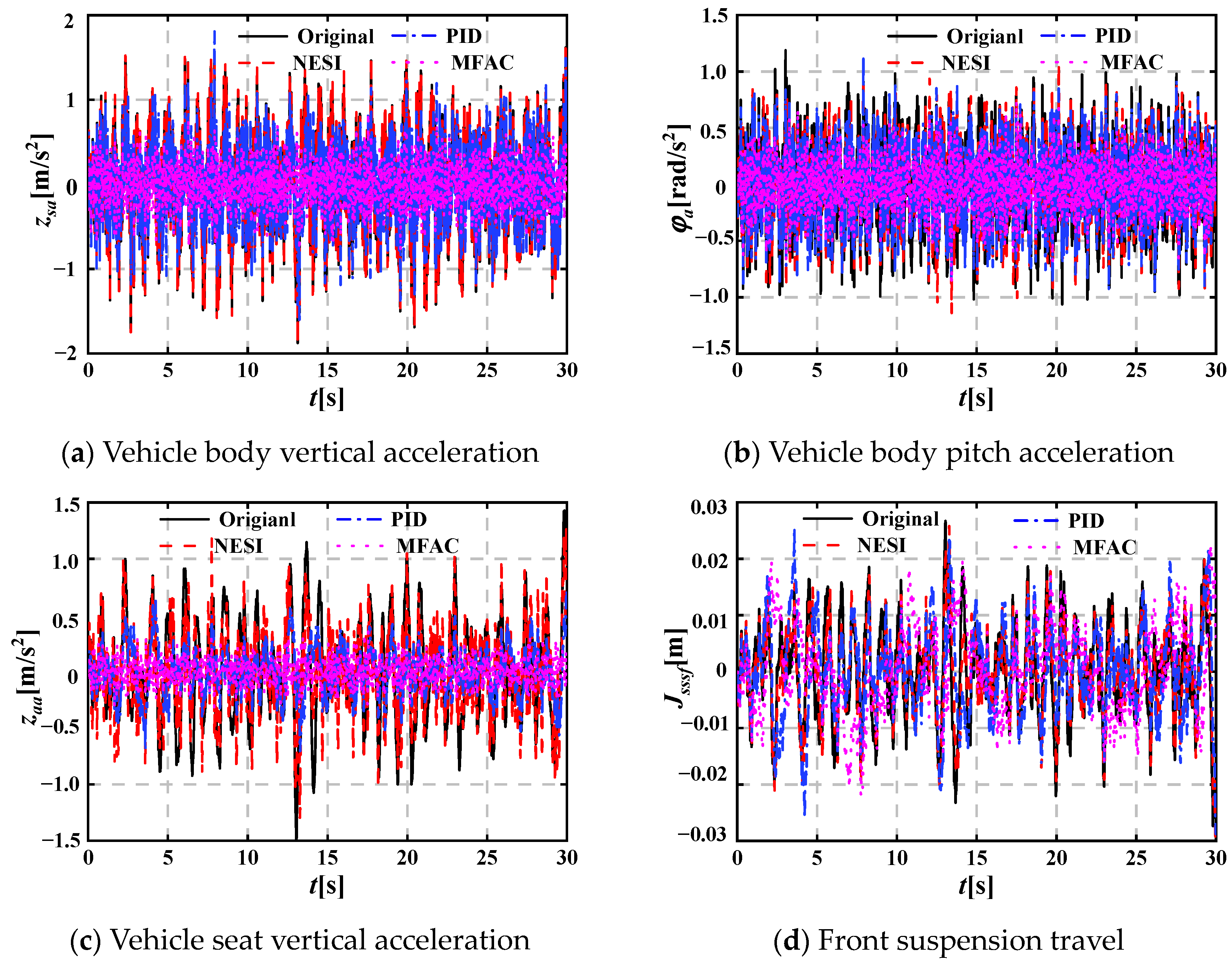
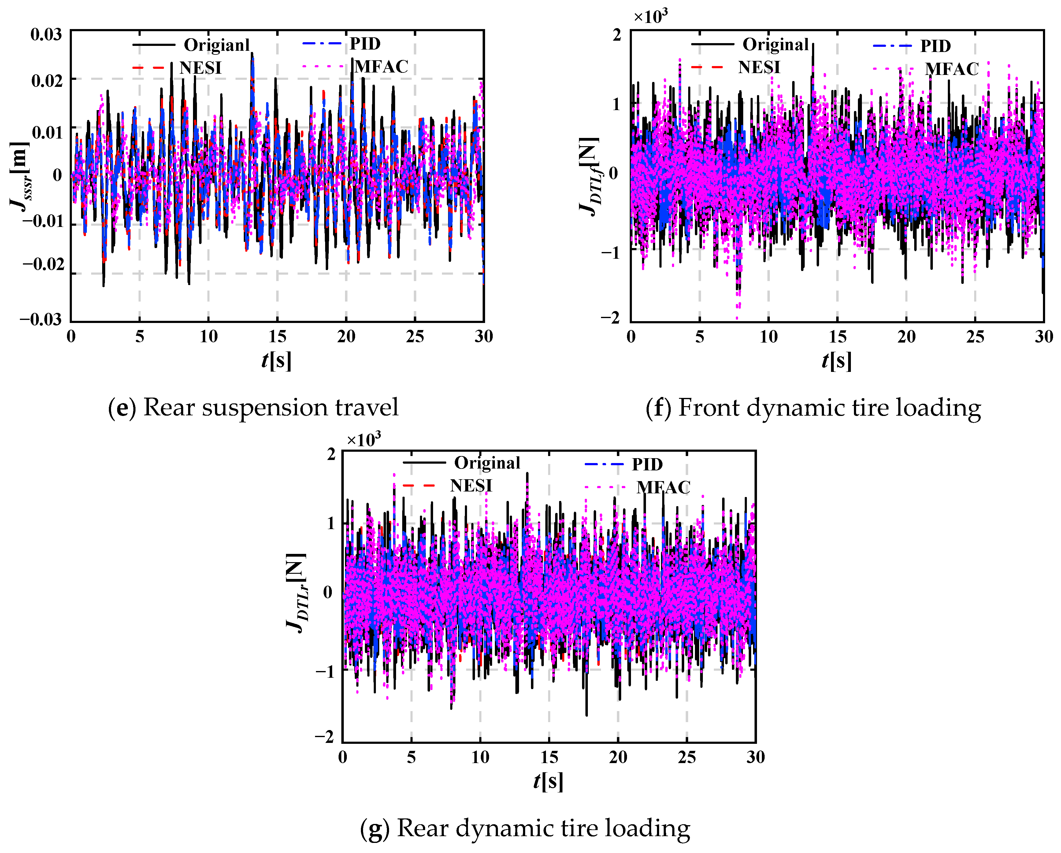
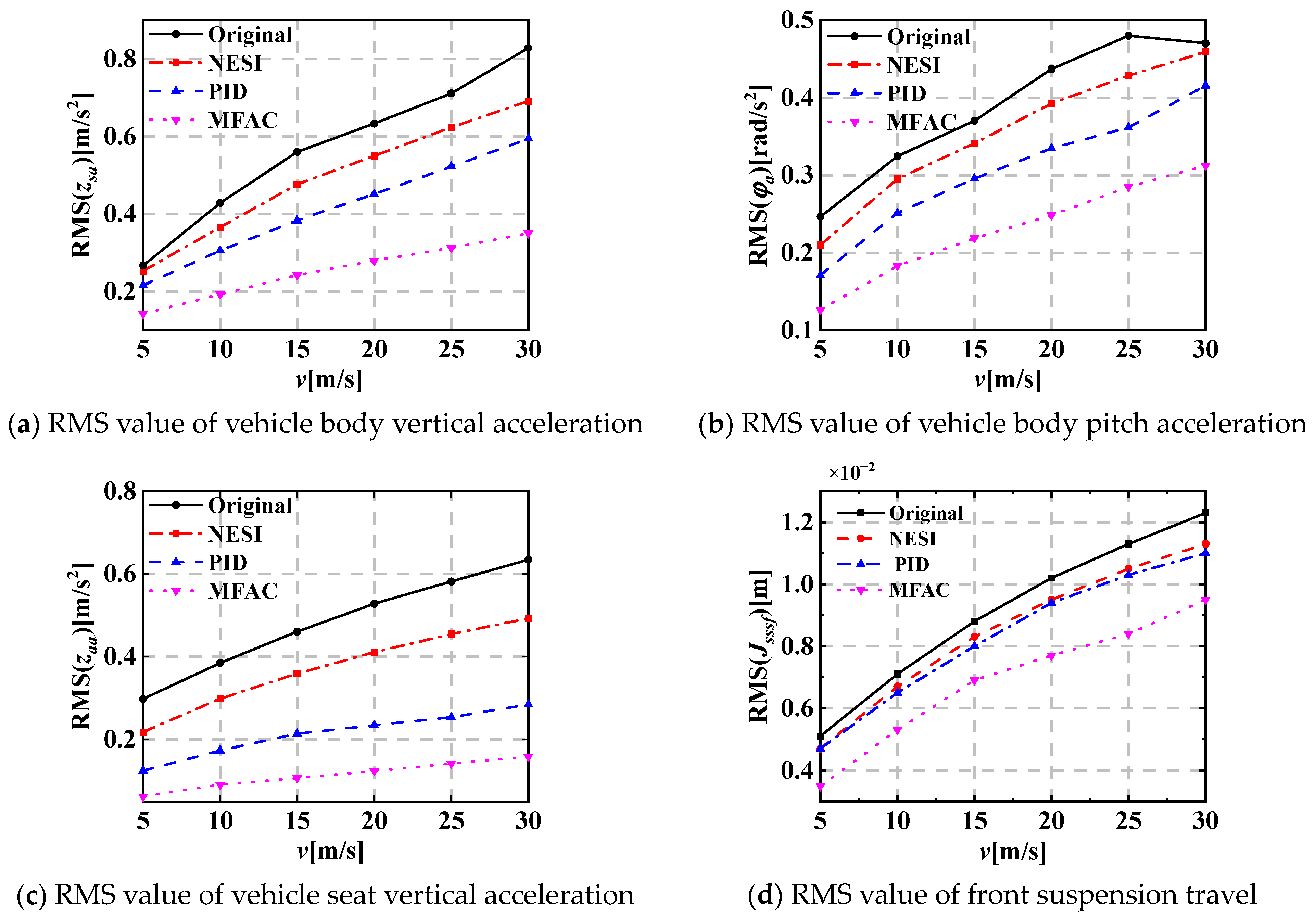
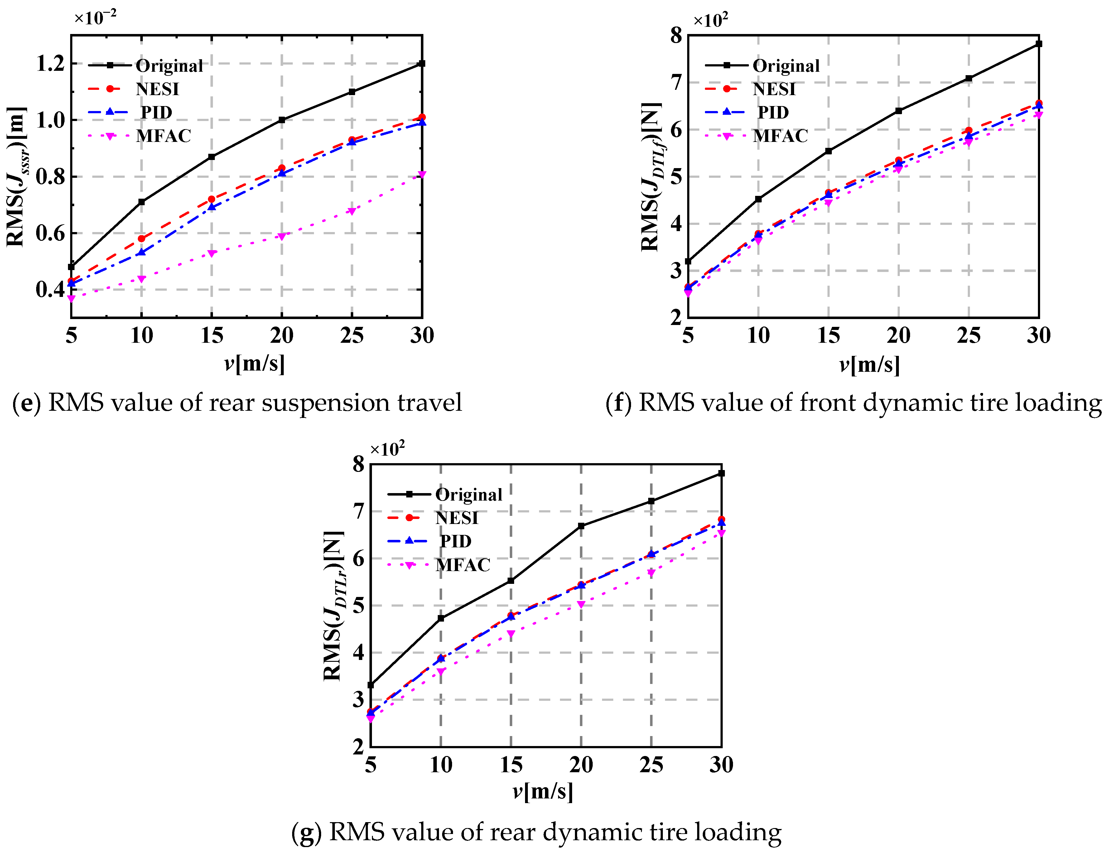
The RMS(z_sa), RMS(φ_a), RMS(z_aa), RMS(J_sssf) and RMS(J_sssr) for the active HVS system coupled with NESI using the MFAC method under random pavement excitation are significantly smaller than those of the original HVS system, the HVS system coupled with NESI, and the active HVS system coupled with NESI using the PID control method; the RMS(J_DTLf) and RMS(J_DTLr) are also slightly smaller than those of the other three HVS systems, which reflects the best dynamic performance among the four HVS systems and demonstrates the effectiveness of MFAC method.

(2)

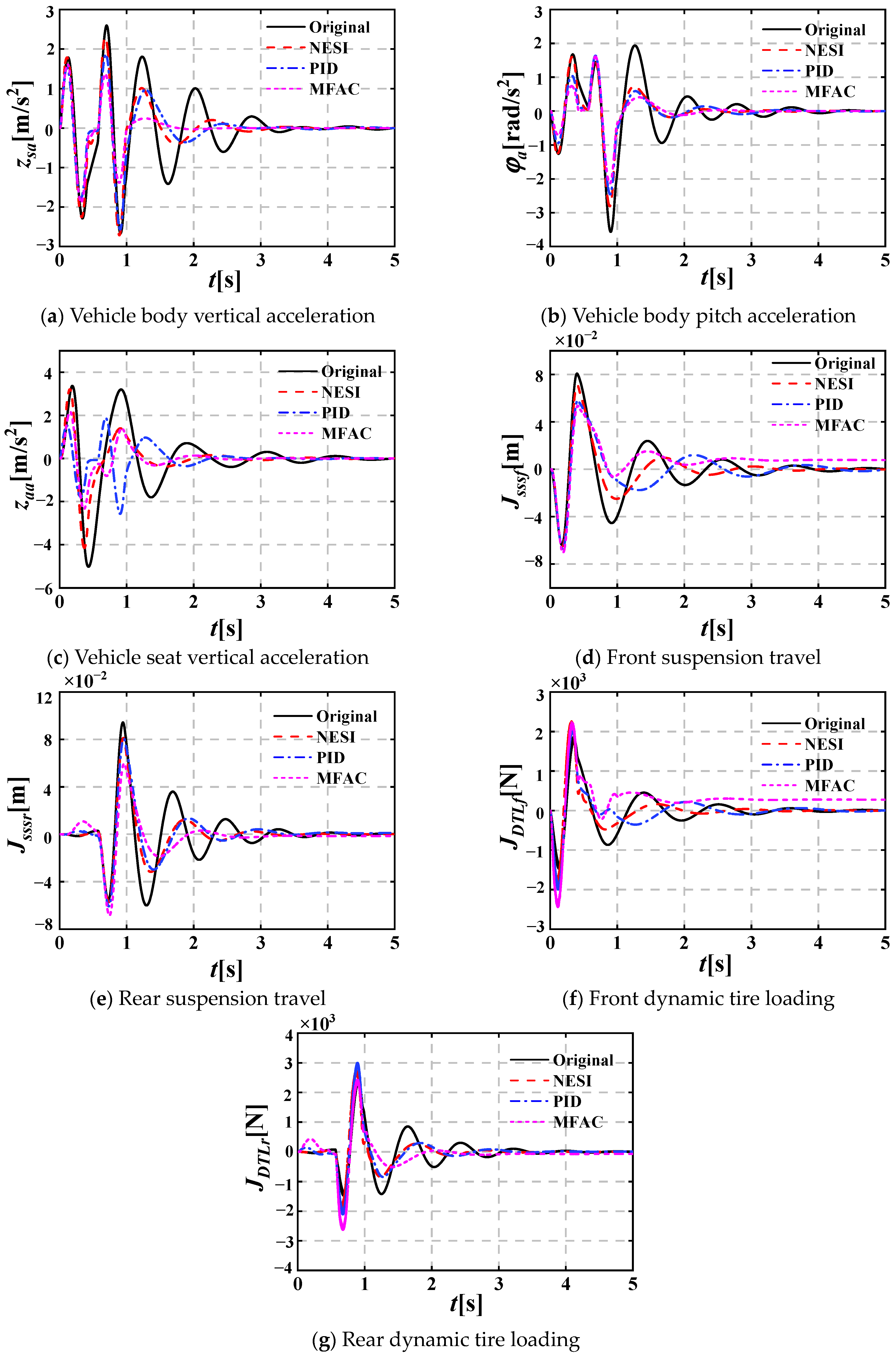
The peak amplitudes of z_sa, φ_a, z_aa, J_sssf and J_sssr for the active HVS system coupled with NESI using the MFAC method under pavement shock excitation are smaller than those of the other three HVS systems, and the vibration attenuation time also shortens; the peak amplitudes of J_DTLf and J_DTLr are larger than those of the other three HVS systems, while the vibration attenuation time decreases, which also shows the benefit of the MFAC method.

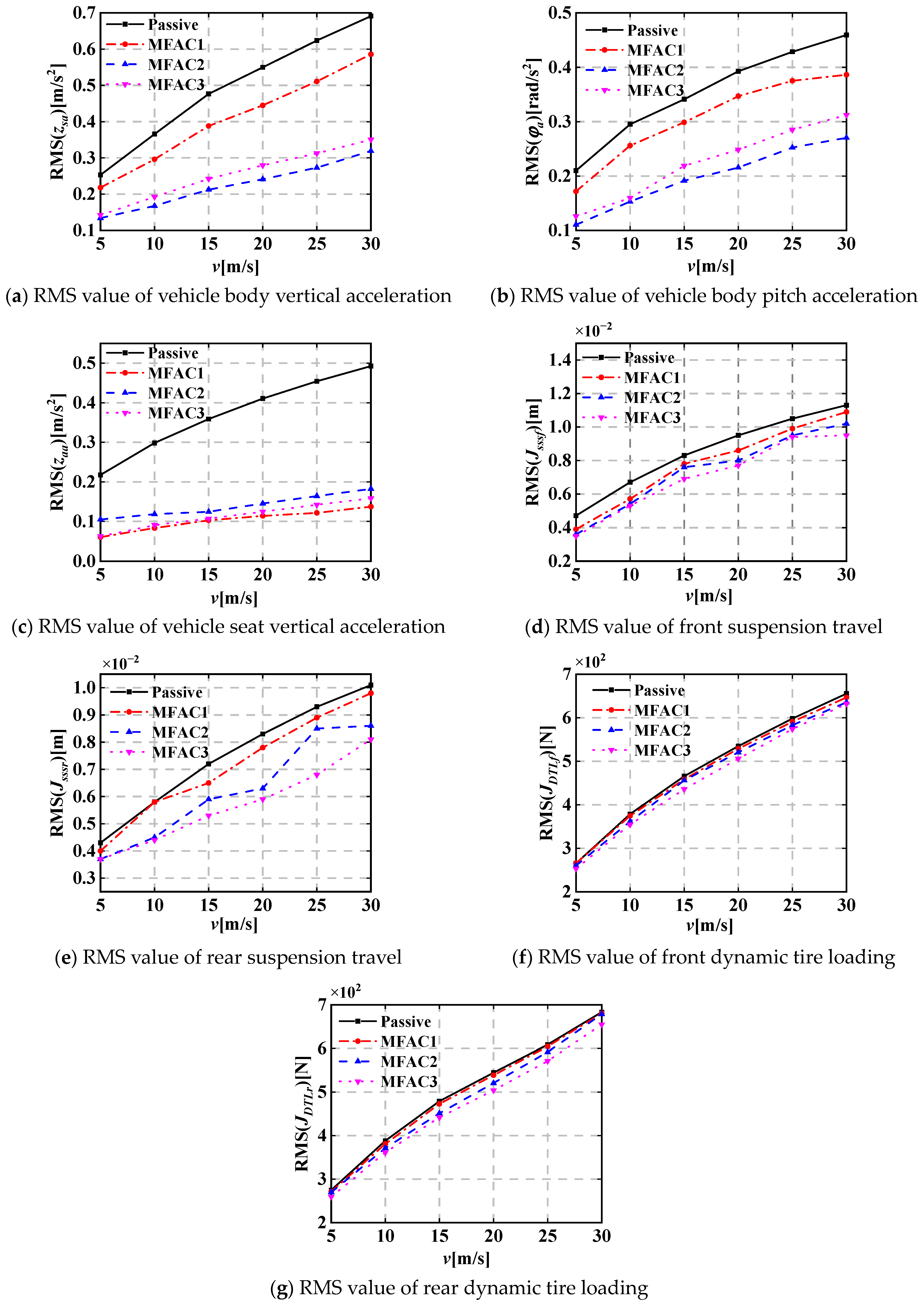
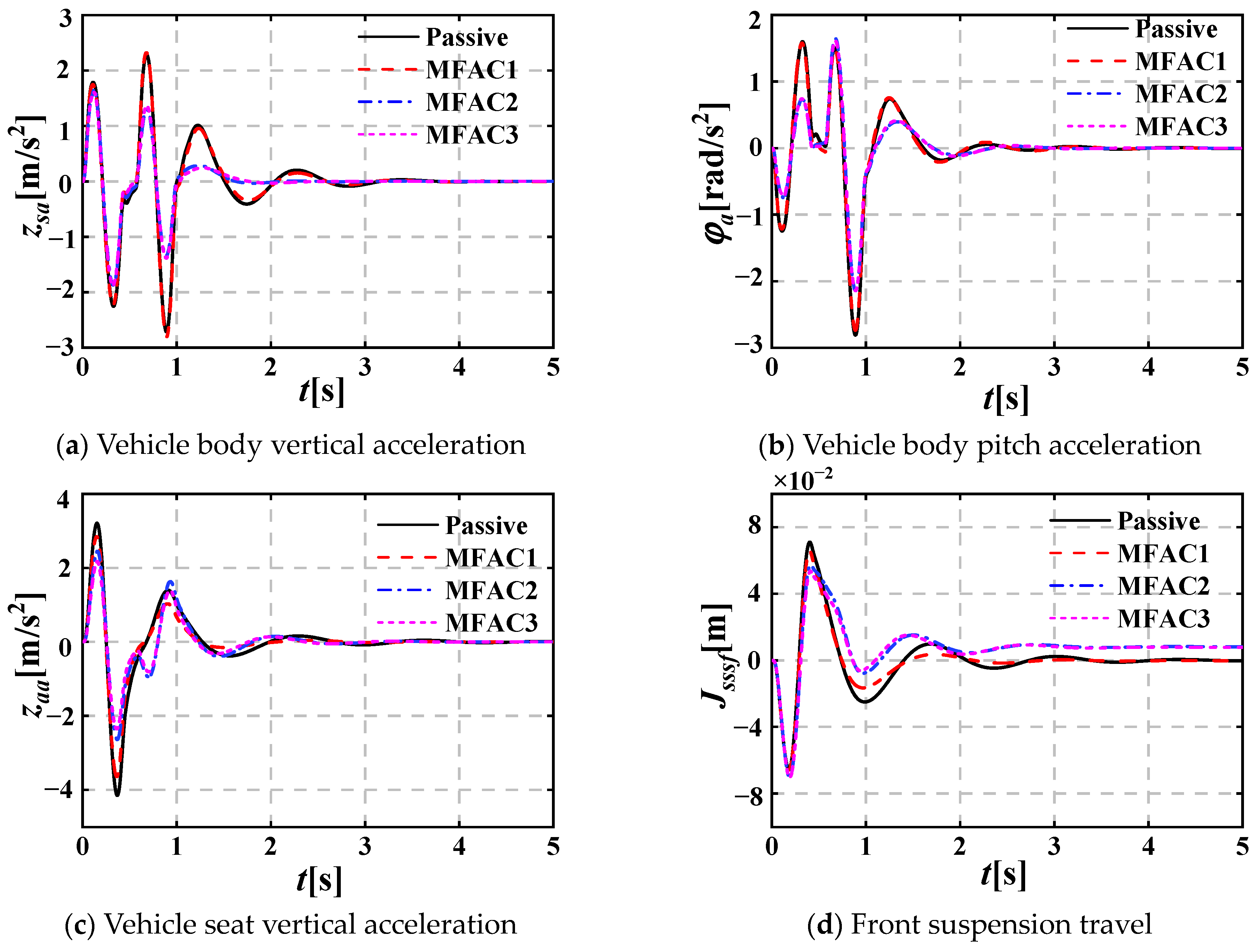
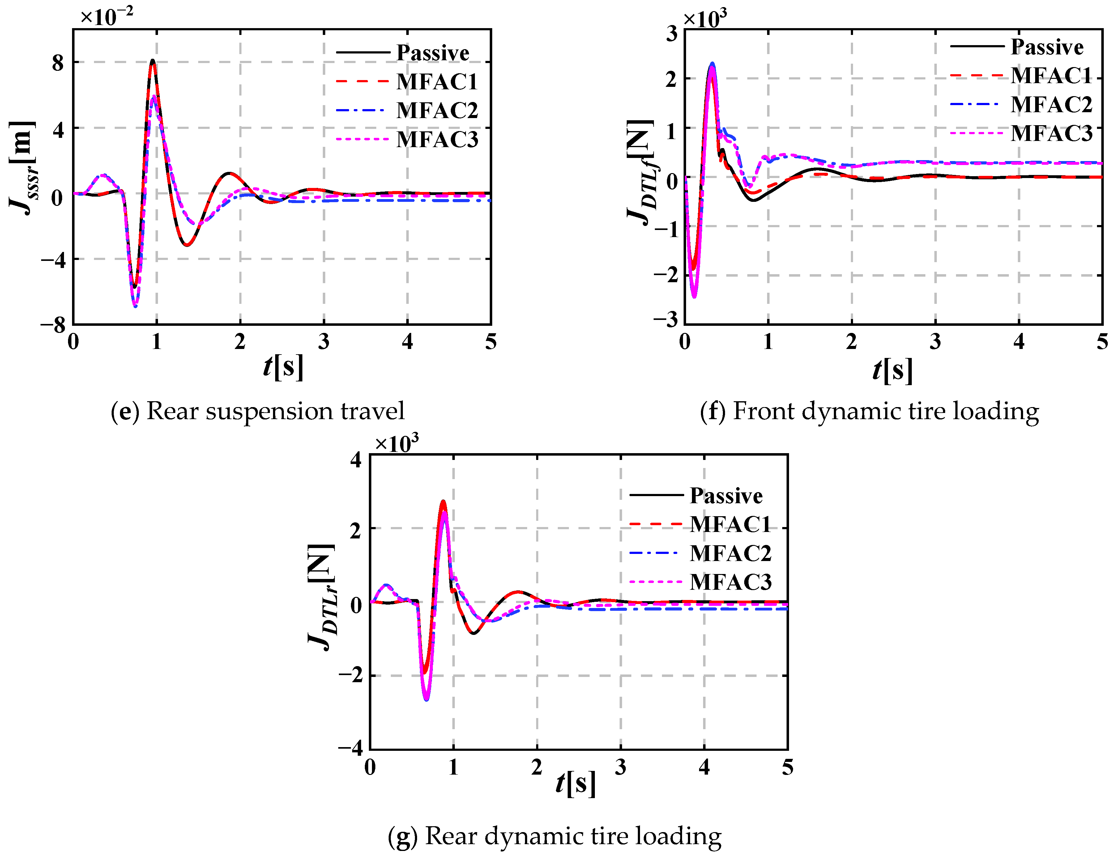
(3)

When the MFAC is acting on both the seat and vehicle suspensions, the active HVS system obtains the best dynamic performance compared with the active HVS system where the MFAC is acting on the seat suspension, and the MFAC is acting on the front and rear suspensions.

Thus, the designed MFAC method can effectively improve the dynamic performance of the HVS system coupled with NESI, which provides guiding significance for vehicle vibration attenuation. In future work, the dynamic characteristics of the full-vehicle-seat system coupled with NESI will be analyzed; the MFAC method will be used in the full-vehicle-seat system to further improve the dynamic performance, and the evaluation criteria of vehicle dynamic performance, including vehicle ride comfort, will be further expanded. Furthermore, experimental research will be carried out to verify the validity of the theoretical results.

References

1. Farshidianfar, A.; Saghafi, A.; Kalami, S.M.; Saghafi, I. Active vibration isolation of machinery and sensitive equipment using H∞ control criterion and particle swarm optimization method. Meccanica 2012, 47, 437–453. [Google Scholar] [CrossRef]
2. Zeng, Y.C.; Ding, H.; Du, R.H.; Chen, L.Q. A suspension system with quasi-zero stiffness characteristics and inerter nonlinear energy sink. J. Vib. Control 2022, 28, 143–158. [Google Scholar] [CrossRef]
3. Ding, R.K.; Wang, R.C.; Meng, X.P.; Chen, L. Research on time-delay-dependent H∞/H2 optimal control of magnetorheological semi-active suspension with response delay. J. Vib. Control 2023, 29, 1447–1458. [Google Scholar] [CrossRef]
4. Wos, P.; Dziopa, Z. Study of the vibration isolation properties of a pneumatic suspension system for the seat of a working machine with adjustable stiffness. Appl. Sci. 2024, 14, 6318. [Google Scholar] [CrossRef]
5. Li, Z.L.; Hou, H.T.; Zhang, Z.; Guo, B.J.; Song, Y.; Liu, Z.Q. Analysis of vehicle ride comfort and parameter optimization of hydro-pneumatic suspension for heavy duty mining vehicle. Eng. Lett. 2024, 32, 2145–2152. [Google Scholar]
6. Li, M.; Li, B.; Chen, G.; Li, H.; Ding, B.H.; Shi, C.Y.; Yu, F. Research on the design and evaluation method of vehicle seat comfort for driving experience. Int. J. Ind. Ergonom. 2024, 100, 103567. [Google Scholar] [CrossRef]
7. Palomares, E.; Morales, A.L.; Nieto, A.J.; Félix, M.; Chicharro, J.M.; Pintado, P. Adaptive optimal control of pneumatic suspensions for comfort improvement of flexible railway vehicles using Monte Carlo simulations. Vehicle Syst. Dyn. 2023, 61, 2790–2810. [Google Scholar] [CrossRef]
8. Kim, J.; Yim, S. Design of a suspension controller with an adaptive feedforward algorithm for ride comfort enhancement and motion sickness mitigation. Actuators 2024, 13, 315. [Google Scholar] [CrossRef]
9. Zhang, S.B.; Li, M.; Li, J.S.; Xu, J.; Wang, Z.L.; Liu, S.H. Research on ride comfort control of air suspension based on genetic algorithm optimized fuzzy PID. Appl. Sci. 2024, 14, 7787. [Google Scholar] [CrossRef]
10. Vakakis, A.F.; Gendelman, O.V.; Bergman, L.A.; Mojahed, A.; Gzal, M. Nonlinear targeted energy transfer: State of the art and new perspectives. Nonlinear Dynam. 2022, 108, 711–741. [Google Scholar] [CrossRef]
11. Ndemanou, P.B.; Ndoukouo, N.A.; Metsebo, J.; Kol, G.R. Nonlinear energy sink response of a cylindrical storage tank under earthquake loads. Soil Dyn. Earthq. Eng. 2024, 179, 108536. [Google Scholar] [CrossRef]
12. Geng, X.F.; Ding, H.; Jin, C.J.; Wei, K.X.; Jing, X.J.; Chen, L.Q. A state-of-the-art review on the dynamic design of nonlinear energy sinks. Eng. Struct. 2024, 313, 118228. [Google Scholar] [CrossRef]
13. Wang, J.; Zheng, Y.; Ma, Y. Movable-track nonlinear energy sinks with customizable restoring forces. Mech. Syst. Signal Process. 2025, 224, 112078. [Google Scholar] [CrossRef]
14. Huang, C.; Zheng, G.; Nie, X.; Yang, G. Supercritical and subcritical aeroelastic behaviors of a three-dimensional wing coupled with a nonlinear energy sink. Int. J. Nonlin. Mech. 2024, 161, 104692. [Google Scholar] [CrossRef]
15. Wang, Y.; Zhang, T.; Bian, H.Y.; Yin, Y.; Wei, X.H. Shimmy performance analysis and parameter optimization of a dual-wheel nose landing gear coupled with torsional nonlinear energy sink and considering structural nonlinear factor. Chaos Soliton Fract. 2024, 187, 115330. [Google Scholar] [CrossRef]
16. Wang, Y.; Zhang, T.; Yin, Y.; Wei, X.H. Reducing shimmy oscillation of a dual-wheel nose landing gear based on torsional nonlinear energy sink. Nonlinear Dynam. 2024, 112, 4027–4062. [Google Scholar] [CrossRef]
17. Wang, Y.; Wang, P.L.; Meng, H.D.; Chen, L.Q. Dynamic performance and parameter optimization of a half-vehicle system coupled with an inerter-based X-structure nonlinear energy sink. Appl. Math-Engl. 2024, 45, 85–110. [Google Scholar] [CrossRef]
18. Zhang, X.L.; Cheng, X.B.; Liu, J.C.; Yang, J.X.; Nie, J.M. Load adaptivity of seat suspensions equipped with diamond-shaped structure mem-inerter. J. Vib. Eng. Technol. 2024. [Google Scholar] [CrossRef]
19. Wang, Y.; Xu, B.B.; Meng, H.D. Enhanced vehicle shimmy performance using inerter-based suppression mechanism. Commun. Nonlinear Sci. 2024, 130, 107800. [Google Scholar] [CrossRef]
20. Smith, M.C. Synthesis of mechanical networks: The inerter. IEEE Trans. Autom. Contr. 2002, 47, 1648–1662. [Google Scholar] [CrossRef]
21. Zhang, Y.W.; Lu, Y.N.; Zhang, W.; Teng, Y.Y.; Yang, H.X.; Yang, T.Z.; Chen, L.Q. Nonlinear energy sink with inerter. Mech. Syst. Signal Process. 2019, 125, 52–64. [Google Scholar] [CrossRef]
22. Zhang, Z.; Lu, Z.; Ding, H.; Chen, L.Q. An inertial nonlinear energy sink. J. Sound Vib. 2019, 405, 34–47. [Google Scholar] [CrossRef]
23. Javidialesaadi, A.; Wierschem, N. An inerter-enhanced nonlinear energy sink. Mech. Syst. Signal Process. 2019, 129, 449–454. [Google Scholar] [CrossRef]
24. Cao, Y.; Li, Z.; Dou, J.; Jia, R.; Yao, H. An inerter nonlinear energy sink for torsional vibration suppression of the rotor system. J. Sound Vib. 2022, 537, 117184. [Google Scholar] [CrossRef]
25. Sui, P.; Shen, Y.J.; Wang, X. Study on response mechanism of nonlinear energy sink with inerter and grounded stiffness. Nonlinear Dynam. 2023, 111, 7157–7179. [Google Scholar] [CrossRef]
26. Wang, Y.; Xu, B.B.; Dai, J.G.; Chen, L.Q. Enhanced dynamic performance of a half-vehicle system using inerter-based nonlinear energy sink. J. Vib. Control 2024, 30, 2857–2880. [Google Scholar] [CrossRef]
27. Zhang, Y.Y.; Ren, C.L.; Meng, H.D.; Wang, Y. Dynamic characteristic analysis of a half-vehicle seat system integrated with nonlinear energy sink inerters (NESIs). Appl. Sci. 2023, 13, 12468. [Google Scholar] [CrossRef]
28. Du, H.; Li, W.; Zhang, N. Integrated seat and suspension control for a quarter vehicle with driver model. IEEE Trans. Veh. Technol. 2012, 61, 3893–3908. [Google Scholar]
29. Lathkar, M.; Shendge, P.; Phadke, S. Active control of uncertain seat suspension system based on a state and disturbance observer. IEEE Trans.Syst. ManCybern. Syst. 2020, 50, 840–850. [Google Scholar] [CrossRef]
30. Han, S.; Dong, J.; Zhou, J.; Chen, Y. Adaptive fuzzy PID control strategy for vehicle active suspension based on road evaluation. Electronics 2022, 11, 921. [Google Scholar] [CrossRef]
31. Hou, Z.; Jin, S. Data-driven model-free adaptive control for a class of MIMO nonlinear discrete-time systems. IEEE Trans. Neural Netw. 2011, 22, 2173–2188. [Google Scholar] [PubMed]
32. Milad, M.; Ioannis, P.; Markos, P. Internal boundary control of lane-free automated vehicle traffic using a model-free adaptive controller. IFAC-PapersOnLine 2021, 54, 99–106. [Google Scholar]
33. Peláez, G.; Alonso, C.; Rubio, H.; Prada, J. Performance analysis of input shaped model reference adaptive control for a single-link flexible manipulator. J. Vib. Control 2024, 30, 5018–5030. [Google Scholar] [CrossRef]
34. Mohammed, A.A.O.; Peng, L.; Hamid, A.H.G.; Ishag, A.M. Disturbance observer-based-model-free adaptive fuzzy fractional-order prescribed performance control for nonlinear PEMFC system with uncertainties and performance constraints. Int. J. Fuzzy Syst. 2024, 1–20. [Google Scholar] [CrossRef]
35. Gu, C.; Tan, C.; Li, B.; Lu, J.; Wang, G.; Chi, X. Data-driven model-free adaptive sliding mode control for electromagnetic linear actuator. J. Micromech. Microeng. 2022, 32, 055007. [Google Scholar] [CrossRef]
36. Du, H.; Zhang, N. Constrained H∞ control of active suspension for a half-vehicle model with a time delay in control. Proc. Inst. Mech. Eng. Part D J. Automob. Eng. 2008, 222, 665–684. [Google Scholar] [CrossRef]
37. Zhang, Y.; Ren, C.; Ma, K.; Xu, Z.; Zhou, P.; Chen, Y. Effect of delayed resonator on the vibration reduction performance of vehicle active seat suspension. J. Low Freq. Noise Vib. Act. Control 2022, 41, 387–404. [Google Scholar] [CrossRef]
38. Wu, K.; Ren, C.; Nan, Y.; Li, L.; Yuan, S.; Shao, S.; Sun, Z. Experimental research on vehicle active suspension based on time-delay control. Int. J. Control 2024, 5, 1157–1173. [Google Scholar] [CrossRef]
39. Mohsen, H.; Shahin, D.; Basohbat, A.; Roshanian, J. On the performance of the model-free adaptive control for a novel moving-mass controlled flying robot. J. Intell. Robot Syst. 2024, 110, 79. [Google Scholar]
40. Hou, Z.S.; Xiong, S.S. On model-free adaptive control and its stability analysis. IEEE Trans. Autom. Contr. 2019, 64, 4555–4569. [Google Scholar] [CrossRef]
41. Liu, D.; Zhang, J.; Lu, X.; Li, C.; Malik, O. Model-free adaptive optimal control for fast and safe start-up of pumped storage hydropower units. J. Energy Storage 2024, 87, 111345. [Google Scholar] [CrossRef]
42. Li, Z.Y.; Cai, S.L.; Li, X.Q.; Shao, S.Y.; Yang, X.Y. Fault diagnosis of rolling bearing for motor based on LSTM-EEMD and genetic optimization. J. Phys. Conf. Ser. 2023, 2549, 012025. [Google Scholar] [CrossRef]
Disclaimer/Publisher’s Note: The statements, opinions and data contained in all publications are solely those of the individual author(s) and contributor(s) and not of MDPI and/or the editor(s). MDPI and/or the editor(s) disclaim responsibility for any injury to people or property resulting from any ideas, methods, instructions or products referred to in the content.
Article Metrics
Citations
Article Access Statistics
Multiple requests from the same IP address are counted as one view.