Robots in Partially Known and Unknown Environments: A Simulated Annealing Approach for Re-Planning

Abstract

The path planning problem using mobile robots, also known as robot motion planning, is a key problem in robotics. The goal is to find a collision-free path from a starting point to a target point in an environment with obstacles. These obstacles can be known, partially unknown, or completely unknown to the robot. The robot’s decisions are different according to its degree of knowledge of the environment. If the environment is fully known, using an offline approach is sufficient. Otherwise, online techniques are required to find a path. They must be fast, effective, and adaptive to tackle the complexity of changing environments. In this work, we propose a framework based on a simulated annealing approach to solve the path planning problem with different degrees of knowledge of the environment for the robot. We evaluate our approach with a set of large-scale instances with different features. The results show that our framework can quickly find quality solutions and is also able to manage environmental changes.

1. Introduction

Robotics is a growing research area in artificial intelligence. The robot motion planning (RMP) problem is a key problem in robotics [1]. The problem concerns mobile robots and consists of finding a path for a robot between two positions and avoiding obstacles. This problem is present in many real-world applications. A mobile robot can be used in situations where humans can be in danger, or places that are not reachable due to the characteristics of the terrain [2].

In this work, we are interested in the motion planning problem when the environment is not fully known. Many offline approaches exist to solve this problem with a known environment [3]; however, it is a new challenge when parts of the environment are unknown [4]. The robot must not only adapt its path to new conditions but also make quick decisions while looking for a minimal path. Our proposal is focused not only on path minimization but also on obtaining smooth paths.

In this paper, we consider a robot with limited sensors that can only detect nearby constraints in its environment such that the robot will discover new areas and new obstacles only when it is moving.

Our motivation is to propose a fast, adaptive, and effective technique for path minimization that can also obtain a smooth path without collision for a robot with limited sensors.

Unfortunately, comparisons with the existing techniques from the literature for online planning are difficult. The authors typically use specific instances of the problem that are neither publicly available nor sufficiently well described to be re-generated. In this paper, we also propose a new publicly available set of instances of robot motion planning for online techniques to have a common set for evaluation.

The main contributions of this work are (i) an adaptation of an offline robot motion approach for solving the online robot motion planning problem, (ii) a framework to solve motion planning problems with different degrees of knowledge of the environment, and (iii) a set of 40 new instances with different degrees of environment knowledge available for new research.

The next section introduces our approach with the environment modelization and the mathematical model of the problem. We roughly present OfflineRMP in Section 4.1, our offline approach, which works in a fully known environment for the robot. OfflineRMP is the basis of our online approach called AdaptiveRMP, which is explained in detail in Section 4.2. Also, we propose a framework to integrate both techniques according to the robot’s knowledge of the environment. We present different instances and testing scenarios in Section 5, as well as the results and a statistical analysis for comparison. We revise the related work and discuss our framework and the results obtained in Section 2. Finally, some conclusions and future work are presented in Section 6.

2. Related Work

Robot motion planning has been studied since 1960. Its original version was the Piano Mover’s Problem, which aims to move a piano or complex object from one room to another with obstacles in the way [5]. The path planning problem is demonstrated to be NP-hard in [6].

Several approaches have been proposed to solve the robot motion planning problem. Most of these are focused on completely known environments, the offline motion planning problem, and the newest ones are focused on unknown environments, the online motion planning version. Moreover, these approaches can be classified as classic methods and heuristic-based methods [7]. Most classic methods can be classified as planning by construction, while heuristic optimization algorithms are classified as planning by modification.

The classic roadmap methods model the space without obstacles onto a network of lines, transforming the offline path planning problem into a graph searching problem. Visibility graphs use the search space to trace lines between different parts of the obstacles. Including the starting and target points, it is possible to create a graph in which a graph search algorithm is used [8]. In these graphs, all the lines must be feasible paths. Voronoi diagrams aim to create graphs of paths similar to visibility graphs, but, instead of using vertices, Voronoi diagrams create additional space around the obstacles [9]. The specific goal considered by these approaches is to obtain the clearest paths.

In cell decomposition approaches, the search space is divided into cells, which are then used to search a path that begins at the starting point and ends at the target point connected by cells in sequence [7]. In potential fields, the robot is treated as a point under the influence of an artificial potential field, while the target attracts the robot, and the obstacles push the robot away [10].

Sampling-based techniques aim to find paths in different samples of the free workspace and then join them [11]. This method obtains good results for robots with a high degree of freedom in static environments. The two main classifications of these methods are probabilistic roadmap methods and rapidly exploring random trees. Probabilistic roadmap methods locate a set of configurations in the free space, which are connected using a local planner. The starting and target positions are added to the path. Finally, a graph-search-based algorithm is used to find the shortest path [12]. A large number of approaches can be found in the literature, all based on the rapidly exploring random trees [13]. The basic method works by iteratively growing a tree from the starting point to the goal node by generating random points in the space that are linked to the closest point in the current tree. The basic algorithm and its variants can be classified as sampling methods. In [14,15], reviews of these RTT methods are presented. Most of the recent approaches consider the use of several trees [16] that enable balancing the processes of the exploration and exploitation of the robot search space by generating random heuristic trees that are used to connect the rooted tree towards the goal area.

In [17], the authors propose a path planning algorithm focused on the consideration of collision risk. The approach combines a trajectory estimation algorithm and A* to select the low-risk points to conform to the path. Also, ref. [18] considers the inclusion of spatial-temporal specifications.

Heuristic algorithms have also been used to solve the offline motion planning problem. In [19], a genetic algorithm is introduced. The goal is to find an adaptable path according to changes in the environment. Each individual of the population corresponds to a candidate solution using a binary representation. In [20], the use of simulated annealing with potential fields is proposed. Once a local minima is found using potential fields, simulated annealing is used with a high initial temperature to enable changing to a worse solution to escape the local minima. In [2], an ant colony optimization algorithm is implemented to solve the offline robot motion planning. In this work, the workspace is discretized in $50\times 50$ connected nodes with binary values representing obstacles. The pheromone levels are initialized at each and change according to the ant’s paths.

In [3], a hybrid approach is presented. Surrounding points set close to critical obstacles are used to find a path, and then particle swarm optimization is applied to improve such a path. When the robot approaches narrow spaces where a feasible path cannot be found, this approach considers more surrounding points, enlarging the grid resolution; if there exists a path, it will be found. The approach can obtain better results than probabilistic roadmap methods [12] and an ant colony optimization-based algorithm [21] solving instances of $2000\times 2000$. In [22], a new hybrid planning algorithm is proposed. The approach, RRT*-CFS, combines sampling-based and optimization-based methods. Here, RRT* [23] is used to construct an initial feasible path, and then the convex feasible set algorithm is applied to solve the non-convex motion planing.

More recently, learning-based approaches have been proposed for the problem. A residual convolutional neural network is proposed in [24]. Inspired by the imitation learning idea, the neural network uses an offline-prepared dataset based on global environment information and the optimal paths for training. An approach for online robot motion planning using neural networks is introduced in [25]. This approach can be used for mobile robots, manipulator robots, and multi-robot systems. Neural networks respond well to changes in the environment related to changes in obstacles or the dynamics of the environment [26]. The instances used include two-dimensional featuress with x and y coordinates and size $50\times 50$ using 2500 neurons to represent the workspace. The instances used include labyrinth workspaces and mobile targets and mobile obstacles.

Machine learning algorithms are coupled with case-based reasoning in [4]. Here, the authors present two approaches that use sets of solutions to resemble new ones using case-based reasoning. Given a path planning problem, the first approach selects a set of similar problems with their respective solutions. These solutions are merged and, using case-based reasoning, a solution to the new problem is constructed. The second approach constructs paths by iteratively analyzing the current state and determining the next ones using case-based reasoning based on the nearest neighbor solutions.

In [27], an evolutionary approach is presented. The approach uses a matrix representation of the workspace where each cell is the size of the robot and movements are restricted to four axes. It solves offline and online planning. For the experiments, small obstacles are included in the initial path. A re-planning of the path is used to avoid collisions. The instances used are from $50\times 50$ to $3000\times 2000$, and the execution times vary from 1 s in the smallest instances to 96 s in the largest instances. The proposed algorithm obtains better results than the classic methods, especially for the largest problem instances. The same authors present in [28] an evolutionary approach for the dynamic problem. In this case, the positions of the obstacles are unknown, and the robot’s sensors are limited. They use the same instances as in their previous work, but the robot only has information on the closest cells. The results vary from 2 s in the easy instances to 250 s in the more complex ones. These results are better in terms of time and the number of re-plannings needed to find a feasible path compared to [29]; however, the length of the path must be improved.

In [30], a convolutionally evaluated gradient first search approach is proposed. A two-dimensional grid is used to model unknown spaces. Convolutional evaluation is used to guide the path to the target location by iteratively evaluating the target orientation. This evaluation enables the algorithm to detect when to move back when continually deviating from the target to avoid spending too much time on failed paths.

More complex autonomous environments like the design of autonomous behavior for humanoid robots require specially designed approaches [31]. Also, data-driven approaches have demonstrated success in these more challenging versions of the problem [32].

Table 1 summarizes the main features of the static environment methods presented here. Historically, the most studied problem has been offline path planning. A large number of the listed studies propose sampling-based/roadmap approaches. As can be observed in Table 1, most of these approaches solve the offline path planning problem. When the online version is studied, heuristic approaches are mostly used. In this work, we propose a simulated annealing algorithm coupled with a surrounding strategy to surpass obstacles. Unlike other online approaches, our method assumes a simple line segment between the start and end points that is made feasible (avoiding obstacles) using the surrounding strategy. When obstacles are detected, the surrounding strategy is applied. Our approach can be used in offline and online scenarios through the framework proposal presented in this research work. Some other strategies have been proposed to solve the offline and online path planning problems. Our proposal describes a simple framework that combines a simulated annealing approach that solves the offline problem with had-doc surrounding strategies to adapt the path to the presence of objects. The approach does not require training time and can be applied without much computational effort to large-size instances with not many objects.

Table 1. Literature summary.

Reference	Year	Approach	Nature	Offline/Online
[8]	1985	Visibility graphs	Roadmap	Offline
[9]	1987	Voronoi diagrams	Roadmap	Offline
[19]	1997	Genetic algorithm	Heuristic	Offline
[13]	2001	Rapidly exploring Random Trees	Roadmap	Offline
[12]	2004	Probabilistic Roadmap	Roadmap	Offline
[20]	2006	Simulated annealing + Potential fields	Heuristic	Offline
[7]	2007	Cell decomposition	Roadmap	Offline
[2]	2009	Ant colony	Heuristic	Offline/Online
[10]	2012	Potential fields	Roadmap	Offline
[21]	2013	Two-phase ant colony optimization	Heuristic	Offline
[3]	2017	Surrounding search+ Particle Swarm Optimization	Heuristic	Offline
[16]	2022	Multi-tree guided RMP	Roadmap	Offline
[18]	2020	Spatio-temporal RRT*	Roadmap	Offline
[22]	2021	RRT*-CFS	Roadmap + Heuristic	Offline
[17]	2021	Trajectory estimation + A*	Heuristic	Offline
[25]	1988	Neural networks	Heuristic	Online
[27]	2005	Evolutionary algorithm	Heuristic	Online
[28]	2008	Evolutionary algorithm	Heuristic	Online
[33]	2018	Firefly algorithm	Heuristic	Online
[34]	2019	Surrounding search	Heuristic	Online
[4]	2020	Machine learning + case-based reasoning	Heuristic	Online
[30]	2022	Convolutionally evaluated gradient first search	Heuristic	Online
Our approach		Surrounding search + Simulated Annealing	Heuristic	Offline/Online

3. Problem Description

In this work, we propose a framework to solve different types of robot motion planning problems according to the environment. These problem instances can be classified as known, partially known, and unknown static instances.

3.1. Environment

In our framework, we use a discrete environment representation. A grid box can have an obstacle or be empty, as shown in Figure 1. In this figure, the starting point is the bottom left corner $(0,0)$ and the ending point is the top right corner $(l-1,m-1)$, where l is the width and m is the height of the grid.

Figure 1. Environment grid. The robot can use one cell at each step. Black cells represent obstacles, and white cells represent free spaces to transit.

From any point on the grid, the robot can move in any of the eight adjacent directions, as shown in Figure 2. Our goal is to find a minimal-distance collision-free path or sequence of movements.

Figure 2. Possible directions for the robot in the grid.

3.2. Mathematical Model

The mathematical model presented in this section is based on [27]. The problem variables enable us to define the route coordinates as follows:

$$x_i=i\text{-}\mathrm{th}\mathrm{coordinate}x\mathrm{of}\mathrm{the}\mathrm{robot},\forall i\in \mathbb{N},x\in \{0,\dots ,l\}.$$

(1)

$$y_i=i\text{-}\mathrm{th}\mathrm{coordinate}y\mathrm{of}\mathrm{the}\mathrm{robot},\forall i\in \mathbb{N},y\in \{0,\dots ,m\}.$$

(2)

The main parameters of the model are related to obstacles. Information related to the presence of obstacles in grids is expressed as

$$O_{x,y}=\left\{\begin{array}{cc}1\hfill & \mathrm{if}\mathrm{there}\mathrm{is}\mathrm{an}\mathrm{obstacle}\mathrm{in}(x,y)\hfill \\ 0\hfill & \mathrm{if}\mathrm{there}\mathrm{is}\mathrm{no}\mathrm{obstacle}\mathrm{in}(x,y)\hfill \end{array}\right.\forall x\in \{0,\dots ,l\},y\in \{0,\dots ,m\}$$

Given that we can work with partially known environments, we consider a parameter to represent obstacles before the algorithm execution. Known obstacles will be represented using a binary matrix with $l\times m$ resolution, where l is the grid width and m is the grid height.

$$Known\_O_{x,y}=\left\{\begin{array}{cc}1\hfill & \mathrm{if}\mathrm{there}\mathrm{is}\mathrm{an}\mathrm{obstacle}\mathrm{in}(x,y)\hfill \\ 0\hfill & \mathrm{if}\mathrm{there}\mathrm{is}\mathrm{no}\mathrm{obstacle}\mathrm{in}(x,y)\hfill \end{array}\right.\forall x\in \{0,\dots ,l\},y\in \{0,\dots ,m\}$$

The main constraints of the problem studied are listed below:

• A robot should change position at each step.

  $$(x_i,y_i)\ne (x_{i+1},y_{i+1})$$

  (3)
• A robot should not use a grid when there is an obstacle.

  $$O_{(x_i,y_i)}\ne 1,\forall (x_i,y_i)$$

  (4)

The main objective of the problem is to find a collision-free path of minimal length. The length of the path is computed by Euclidean distance. The objective can be represented as

$$\mathrm{Minimize}L\left(P\right)=\sum _{i=1}^{n-1}\parallel P\left(i\right)-P(i+1)\parallel$$

(5)

where P represents the constructed path, each $P\left(i\right)$ represents the i-th position of the robot during the path, and n is the number of positions of the path. The norm operator computes the Euclidean distance between two positions in sequence. Each position is described by its horizontal and vertical coordinates on the map.

4. AdaptiveRMP Framework

The framework proposed, AdaptiveRMP, includes different components that work as shown in Figure 3. Depending on the environment detected, subsets of components are used. These components are explained as follows.

Figure 3. AdaptiveRMP components. According to the environment type identified: known, partially known, or unknown; the framework selects the algorithm to use.

4.1. OfflineRMP

This planning scenario searches for a feasible path for the robot navigating from the start to the target position in a known environment. A simulated annealing algorithm proposed in [35] is used to solve this problem. In this algorithm, solutions are presented as coordinates representing the sequence of positions the robot must follow from the start to the target. The simulated annealing approach works in the feasible space; hence, solutions that use obstacle positions are not considered.

Algorithm 1 shows the main structure of the OfflineRMP algorithm implemented. Table 2 summarizes the main symbols used to describe the algorithm. It lists the SA-related symbols as initial and current temperature and differences in the quality of solutions. It also lists the solution points of the paths being constructed.

Table 2. Symbols.

Name	Description
start	initial point of the path
target	final point of the path
$t_0$	initial temperature of simulated annealing
t	current temperature of simulated annealing
$p_1$	initial point of the path to modify
$p_2$	final point of the path to modify
$\Delta$	difference in quality between current and new paths

The SA algorithm implements two main steps: the pre-processing and the search. Before the initial solution is constructed, the empty cells that the robot cannot reach are marked as obstacles using the flood-fill algorithm [36] (line 1). Figure 4 shows the grid obtained after the flood-fill algorithm.

Algorithm 1 OfflineRMP

1: flood_fill(obstacles); 2: if $thereisapath$ then 3:    route = direct_route(start, target); 4:    initialize_temperature($t_0$); 5:    $t=t_0$; 6:    while $maximumiterationsnotreached$ do 7:      ($p_1$, $p_2$) = select_random_coordinates(route); 8:      new_route = generate_new_route($p_1$, $p_2$); 9:      if len(new_route) < len(route) then 10:         route = new_route; 11:      else 12:         acceptance_criterion($\Delta$, t); 13:         if new_route is accepted then 14:           route = new_route; 15:         end if 16:      end if 17:      decrease_temperature(t); 18:    end while 19:    post_processing(route); 20:    return route; 21: else 22:    return (“There is no possible route between start and end points”); 23: end if

Figure 4. Obstacle filling. The flood-fill algorithm fills inaccessible positions inside obstacles.

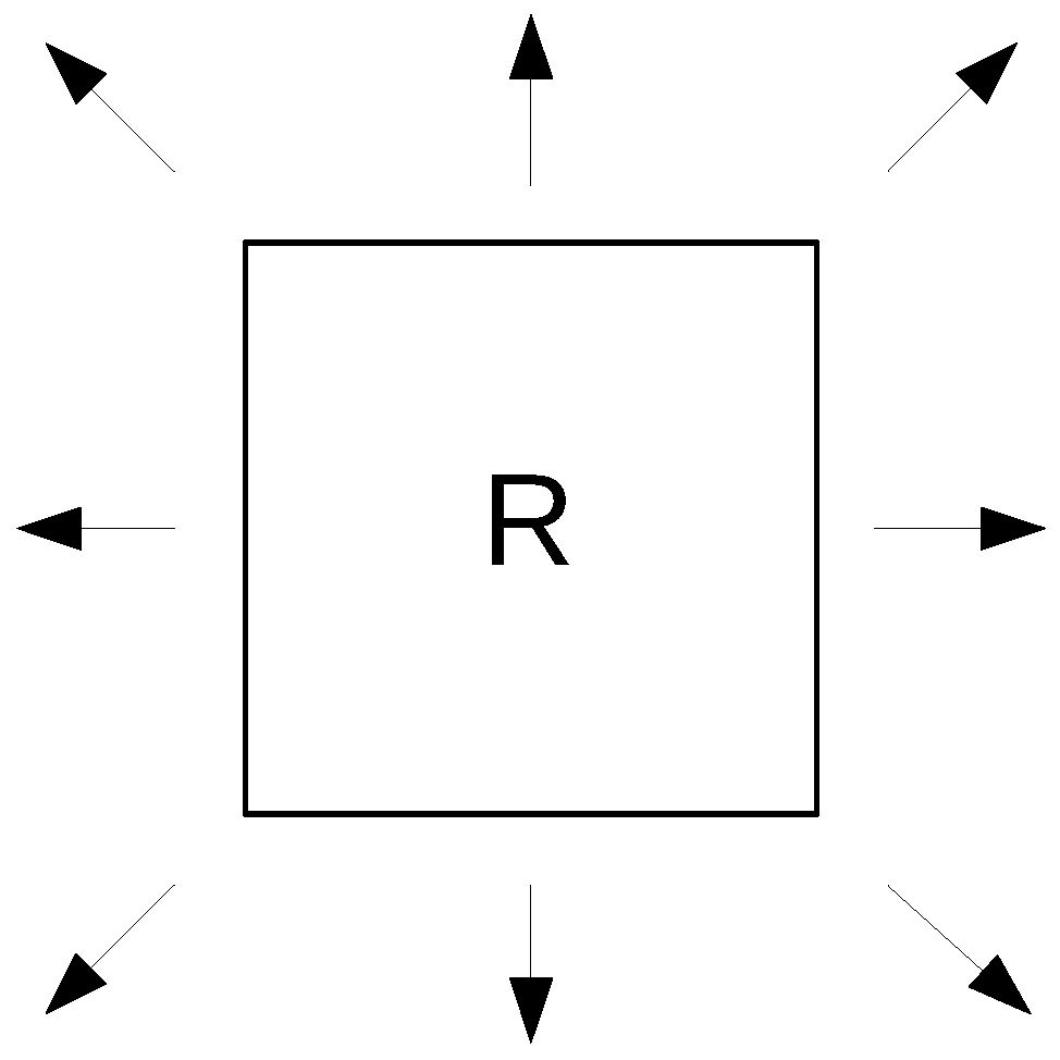
A greedy-based approach generates initial solutions (line 3). The approach uses a myopic function, a pile of directions, a surrounding strategy, and a pruning strategy. The myopic function detects the possible movements to perform in the next step without violating the constraints defined in Section 3.2. The next step is a selection based on the priorities defined by the pile of directions. The robot follows the direction without obstacles approaching the target cell. When an obstacle is detected, the algorithm selects to surround the obstacle by left or right. After this, the robot follows its path using the same strategy.

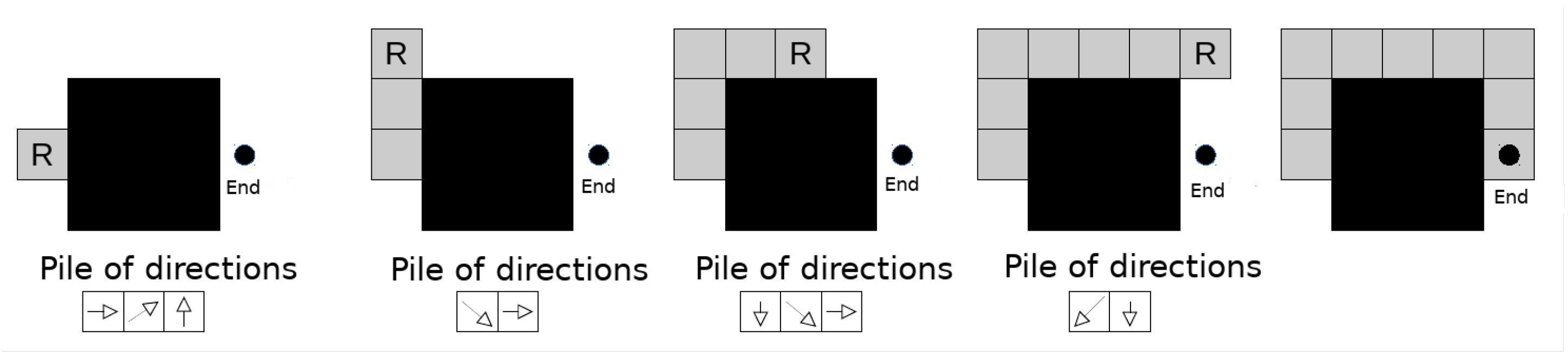
During the surrounding step, the pile of directions defines the priorities of selecting the next position, considering that, at any point, the robot has a suitable direction. If the robot is going around an obstacle, the suitable direction is the one that guides it closer to the obstacle. Otherwise, the suitable direction is the one that brings the robot closer to the destination cell. If an obstacle is being surrounded, the positions are searched starting from the suitable direction counterclockwise. Otherwise, the positions are searched from the suitable direction clockwise.

Figure 5 shows the surrounding strategy. In this case, it has been chosen to surround the left. Hence, positions are added to the pile, starting with the suitable direction until a feasible position is found. The pile is computed in each step according to the current suitable direction. A pruning strategy is included to discard unfeasible surrounding steps. Once an unfeasible step is detected, a new surrounding strategy is selected.

Figure 5. Piles of directions. The first option in each pile considers the center of the obstacle.

The local search phase (lines 6–18) uses a move to repair the candidate solution (line 8). The route between two randomly selected positions from the current path is replaced by a new sub-path that joins these two positions. If there are no obstacles between these positions, a linear sub-path that joins them is generated. If there are obstacles, for each obstacle, the algorithm decides either to surround it by the left or the right, generating an alternative candidate solution.

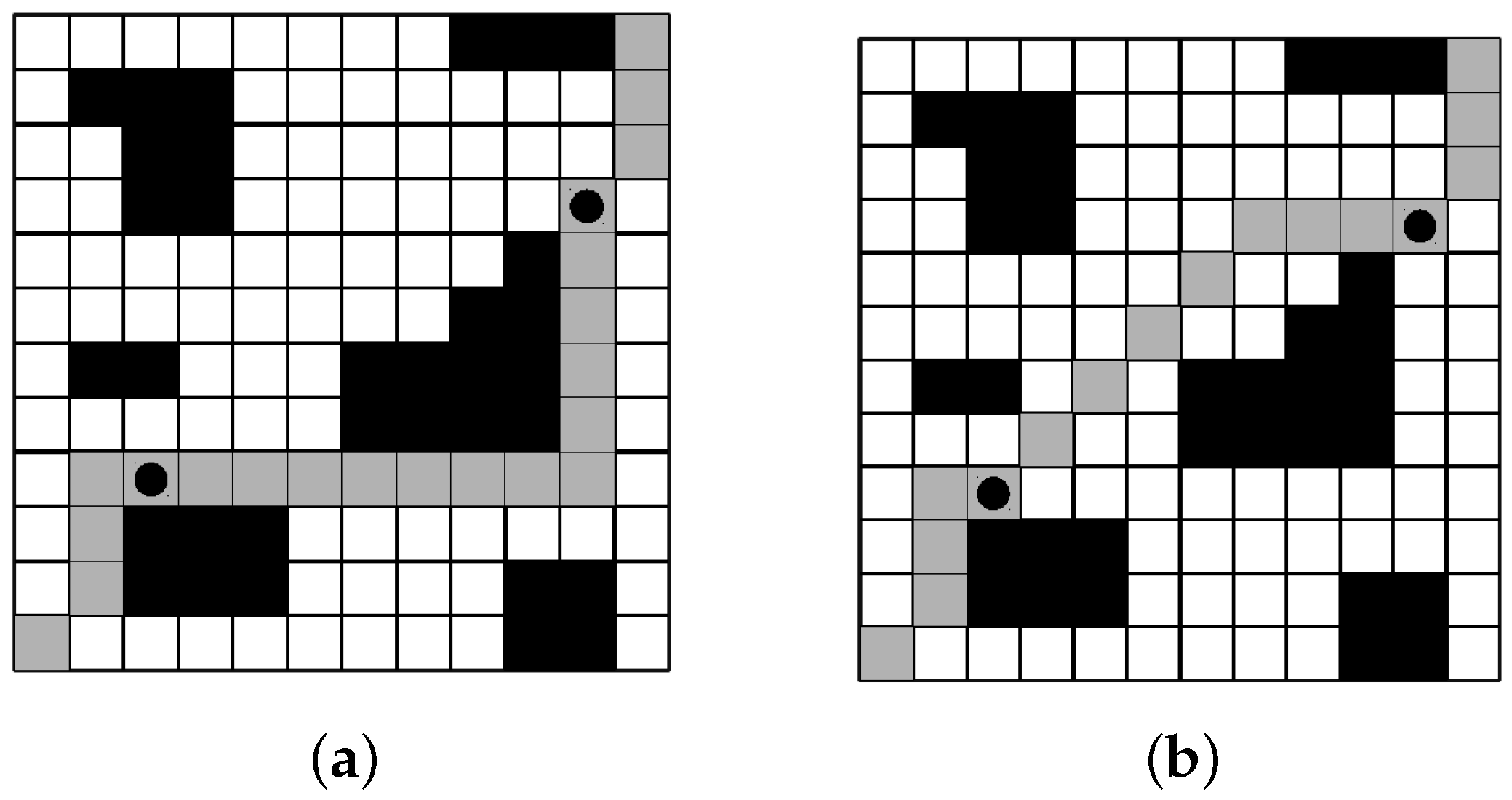
Figure 6 shows a situation without obstacles between the two selected positions marked with circles. Gray grids show the current path in (a) and the new path in (b). A direct sub-path is selected.

Figure 6. Applying the movement of SA without obstacles. The current solution is shown in (a), and the new solution obtained is shown in (b).

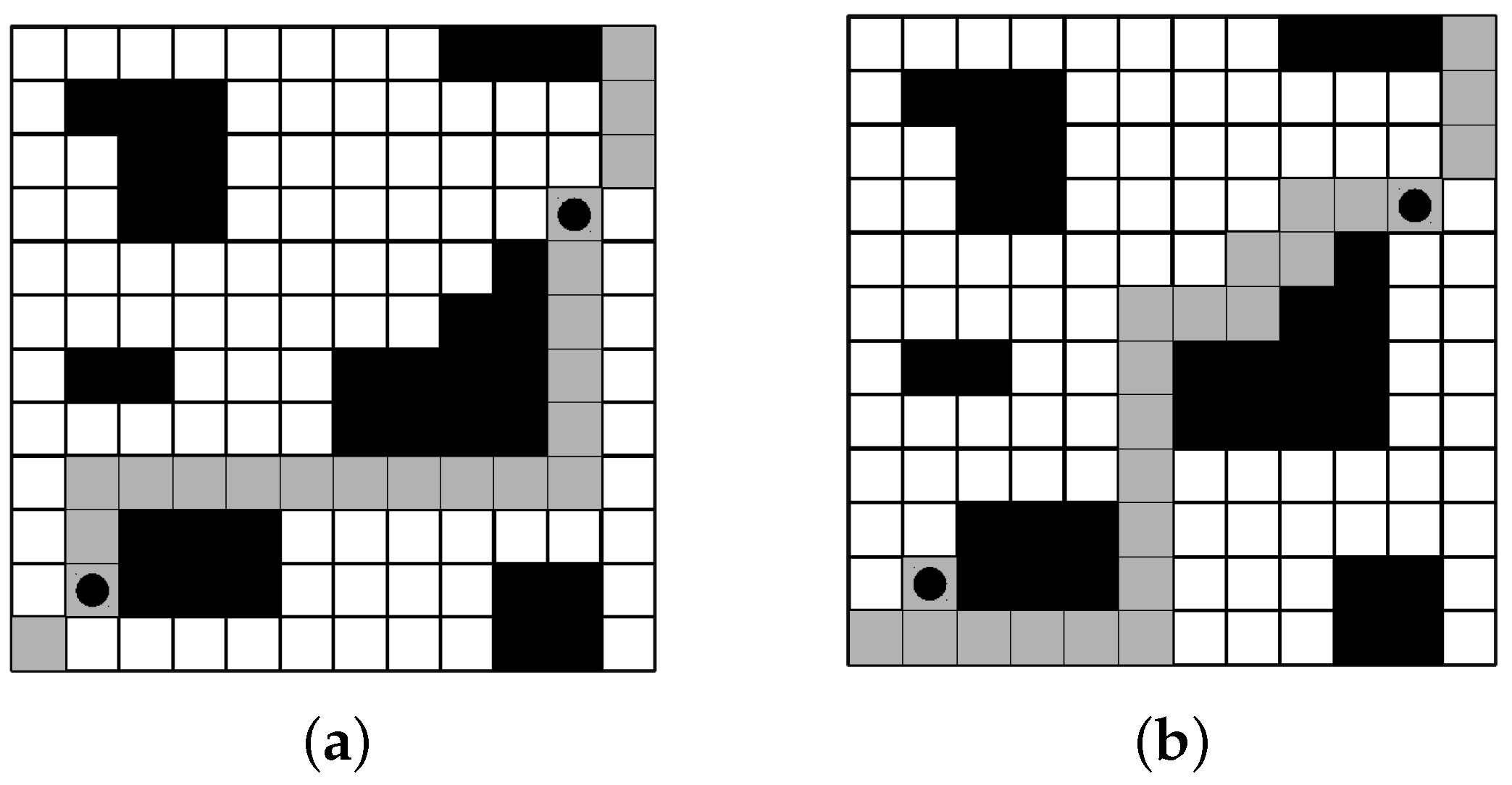
Figure 7 shows an example of obstacles between the two selected positions. As in Figure 6, circles show the randomly selected positions, the current path is shown in gray in (a), and the new route is shown in gray in (b). In this example, it is randomly decided to go around the right of the first object. The second obstacle is surrounded on the left.

Figure 7. Applying the movement of simulated annealing with obstacles. The current solution is shown in (a), and the new solution obtained is shown in (b).

If the new route is shorter than the previous one, it is accepted and selected as the current solution for the next iteration. If the new route is longer than the current one, the probability computed by $e^{-{\displaystyle \frac{|\Delta |}{t}}}$ is used to determine if it should be accepted as the current solution or not.

A post-processing step is used to improve the quality of the paths obtained in terms of length in line 19. The post-processing algorithm follows the path from the beginning and tries to join its current cell to the farthest collision-free cell with a straight line. The final path is constructed by joining the vertices of the path.

Figure 8 shows a solution path before the post-processing (a) and after the post-processing step (b). Here, the start and target cells are in blue, the solution path is in red, and the obstacles are in gray.

Figure 8. Solution generated for back_and_forth instance before post-processing in (a) and after post-processing in (b). Blue circles represent the start and target positions. Obstacles are shown in gray and the route is shown in red.

This move generates diverse solutions without traversing the entire environment. This prevents it from going around obstacles that are not in its way. Surrounding obstacles when close to colliding makes it easiest to return to the original path and follow to the ending point. Direction choice is also important in going around an obstacle. Otherwise, it would be more difficult to return to the original path.

Post-processing increases the degree of freedom the robot has without being restricted by the discretization of space. In addition, the number of times the robot rotates is decreased.

4.2. OnlineRMP

The goal of OnlineRMP is to find a feasible route for the robot to navigate from a starting point to a target point in an environment where the location of obstacles is entirely unknown. Because planning is performed in real time, it is essential to perform it in low execution times.

The same representation of OfflineRMP is used for OnlineRMP.

Because information about the environment is not always known, path planning in real time is closer to reality, where the robot collects information from the environment on the fly and re-plans the path if necessary.

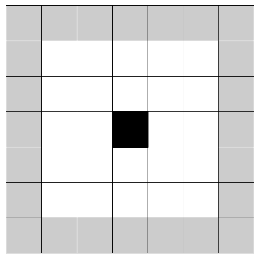
To solve the planning problem in an unknown environment, initially, the robot has the information in the map resolution and the starting and ending positions. Sensors enable the robot to discover two cells around it, as shown in Figure 9. Here, the robot is shown in black, white cells show the space that can be observed by the robot, and, in gray, those that are out of sight are shown.

Figure 9. Robot vision range. White cells are visible to the robot, while gray cells are out of sight.

A greedy method is used to construct initial solutions. For the construction of a path between two positions, the surrounding strategy, the pruning of non-feasible sub-path, and the pile of directions used by the OfflineRMP are also adapted.

As the robot advances, information about the environment is updated with its available vision range. In this case, it can create an unfeasible solution given the unknown obstacles. If the robot is close to colliding, it will be necessary to re-plan the path. It is important to note that the re-planning of the path will occur only on the remaining path and up to the length of the obstacle that is within the current vision range. Because the planning is performed in real time, the path already traveled cannot be modified. Moreover, since the remainder of the way is unknown, re-planning the path to the end is forbidden. Once the re-planning is performed, the robot advances until it is close to colliding with a new obstacle, generating a new re-planning. This continues until the robot reaches the ending point or it cannot continue because an obstacle is found.

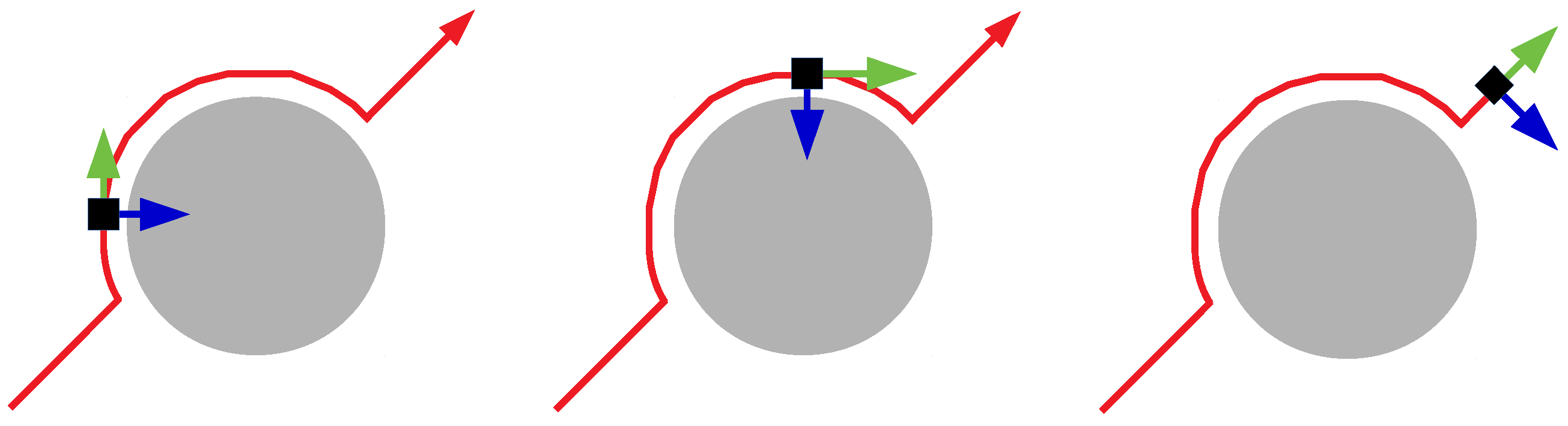
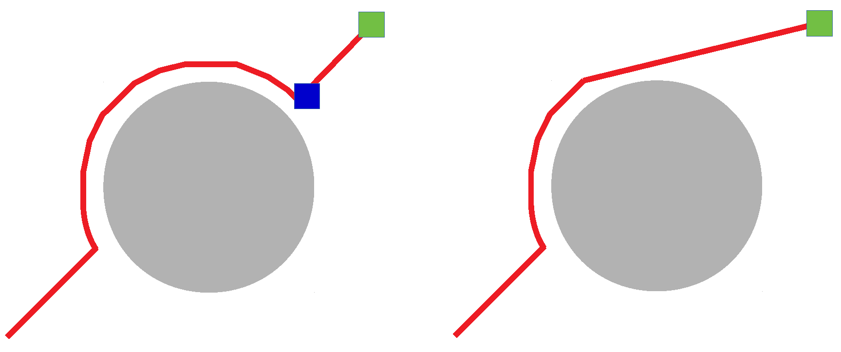
Given the limited vision of a robot, only a portion of the obstacle may be known when using the surrounding strategy. When new information is available, the robot will decide to go around to the object from the right or the left. This can cause the robot to become caught. For this, the normal vector for the movement direction and the obstacle is considered. Figure 10 shows the surrounding change as the robot moves around an obstacle. The black square represents the robot, the obstacle is in gray, and the path is in red. The current direction and its normal vector are shown in green and blue, respectively.

Figure 10. Use of normal vector concerning the direction for obstacle surrounding in real time.

At each step, the normal direction is verified pointing to the obstacle; if it is, then the previous orientation of the surrounding strategy is maintained. If the normal direction is not pointing to the obstacle at any moment, the robot is no longer circling the same obstacle. In this case, the next re-planning of a new surrounding orientation may be random.

Because the flood-fill algorithm described in Section 4.1 is expensive for high-resolution instances, it is used only in the case when the robot tries to go around an obstacle and the two orientations (left or right) are unfeasible. In this case, the robot follows an unfeasible path, so flood-fill is used. It can also be used when the robot tries to go around an obstacle and reaches the same point from where it started; that is, an obstacle surrounds the target point.

As the robot moves around an obstacle, it maintains a local goal of target; once it is possible to reach the final goal via a direct path, that path is used, and the local target of the surrounding strategy is discarded. In Figure 11, two cases of detour are shown. The obstacle is represented in gray, the generated path in red, the final objective in green, and the local objective in blue. On the right, the discarding is used, and, on the left, the surround is completed.

Figure 11. Route generated by going around the obstacle without discarding a local target on the left and discarding it on the right.

Algorithm 2 shows the general structure of the planning approach for an unknown environment using the constructive method. Before traveling the path in real time, an initial route is built considering the known partial obstacles. For this, the SA-based approach for OfflineRMP previously described is used. Since OnlineRMP uses a discretized environment and the path generated by OfflineRMP must be traversed cell by cell, OfflineRMP is used without applying post-processing. The procedure shown in Algorithm 2 starts by constructing an initial solution that defines a direct path between the start and end positions in line 1. Then, the robot starts moving and checking each position in the initial path. From the sensors, the robot can update the information about obstacles in the route in line 3. When a possible collision is detected, re-planning is performed (line 5). Details of the re-planning process are shown in Algorithm 3. Here, when it is possible to reach the final goal via a direct path, then that path is used, and the local goal of the surrounding is discarded. Once a re-planning process is performed, the algorithm resumes the initial path.

Algorithm 2 OnlineRMP

1: route = direct_route (start, target); 2: for position in route do 3:    update_obstacles_map (); 4:    if is close to collision then 5:        route = Re-planning (position); 6:    end if 7: end for

Algorithm 3 Re-planning

1: path_to_fix = obstacle_length(); 2: if direct_route (position, local_target) then 3:     route = direct_route (position, local_target); 4:     new_route = surround_obstacle (position, path_to_fix); 5: else 6:     path_to_fix = obstacle_length (); 7:     route = surround_obstacle (position, path_to_fix); 8: end if

Because OnlineRMP is an algorithm that works in real time, each position the robot moves will be part of the final route. Once the current sub-path is finished, the robot follows the original path. Re-planning is performed as many times as necessary until the target point is reached or when there is no feasible path.

4.3. AdaptiveRMP

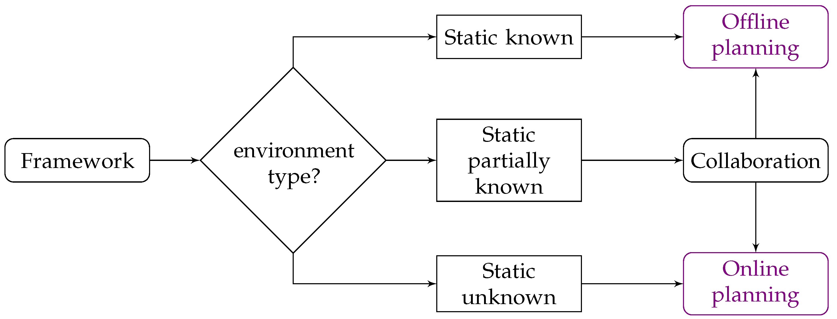
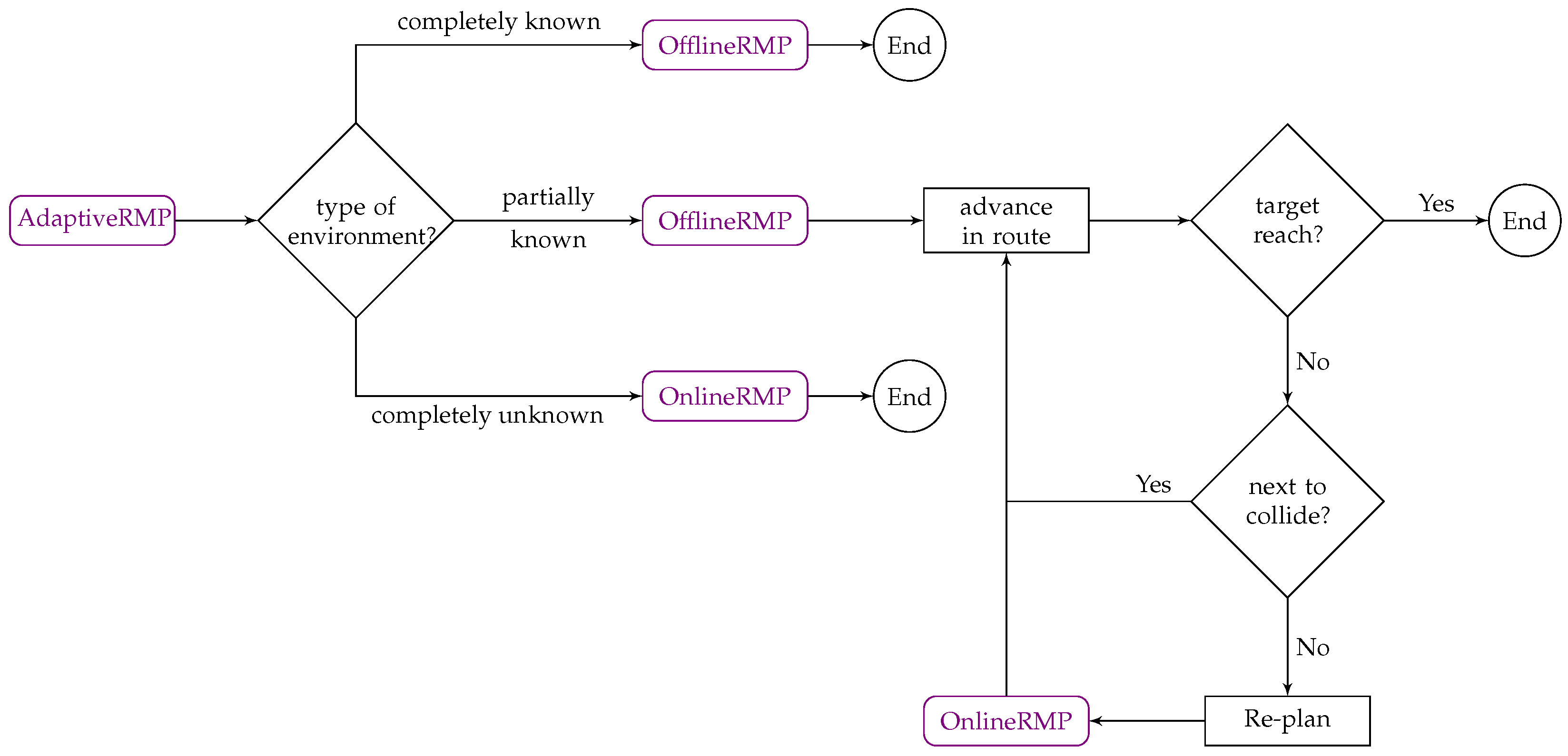
AdaptiveRMP is a cooperation of the two previously described approaches. Figure 12 shows a flow diagram of AdaptiveRMP. According to the features of the environment, OfflineRMP and OnlineRMP are used for completely known and completely unknown environments. In the case of partially known environments, the framework first performs OfflineRMP and then advances along the route until the target is reached or the robot is next to collide. Each time the robot is next to collide, the framework changes to OnlineRMP on the specific segment to re-plan and then continues the path. For this, the new information in the environment is considered, computing a route re-planning range. It is also necessary to return to the route previously generated by OfflineRMP once the route to the new obstacle is discovered. To achieve this, a selection of the section to be re-planned is used, from the current position of the robot to the furthest cell from the original path that can be reached with a direct path without collision; this is conducted without taking into account obstacles recently discovered. Once the section to be re-planned is obtained, the OnlineRMP algorithm is used again.

Figure 12. Flow diagram of AdaptiveRMP.

5. Experiments and Results

In this section, the instances used and the test setup are presented. Our algorithms were implemented in C++ and compiled with gcc. The tests were executed on an Intel(R) Core(TM) i7-2600 CPU @ 3.40 GHz with 16 GB of RAM under a Ubuntu 14.04 distribution.

5.1. Instances

The instances used to test the algorithm were selected from the Intelligent and Mobile Robotics Group’s web page (http://imr.ciirc.cvut.cz/planning/maps.xml (accessed on 12 November 2024)). The set contains nine instances with various sizes and obstacle quantities; the details are shown in Table 3. These are well-known problem instances from the literature that enable a comparison with several previous studies. These instances are different in terms of the number of obstacles, shapes of obstacles, size of the map, and narrowness of roads that enable us to validate the performance of our approach in structurally different problem instances.

Table 3. Instances’ details.

ID	Name	Resolution	Obstacles
(a)	back_and_forth	2000 × 2000	4
(b)	corridor_wavy	2000 × 1800	2
(c)	bugtrap1	1300 × 1000	1
(d)	clasps	2000 × 2000	4
(e)	complex	2000 × 2000	7
(f)	potholes	2000 × 2000	23
(g)	rockpile	2000 × 2000	25
(h)	var_density	2000 × 2000	42
(i)	square_spiral	2000 × 2000	2

We used the experimental setup proposed by Han and Seo in [3], where starting and target positions are randomly chosen. Each configuration was tested with 30 different seeds, and the average and standard deviation were considered. Instances are shown in Figure 13.

Figure 13. Instances.

Given the variety of environments, the instances selected can be classified into three main types:

• Polygonal obstacles: Obstacles with regular and continuous edges. Shown in Figure 14a.
  

  Figure 14. Environments’ variety.
• Irregular obstacles: Obstacles with irregular edges. Shown in Figure 14b.
• Labyrinth: Instances with narrow passages, often with one entry and one exit. Shown in Figure 14c.

5.2. OfflineRMP Analysis

The OfflineRMP component performance was studied in [35]. Moreover, here, we performed a tuning procedure to determine the best parameter values for the simulated annealing approach and their component relevance.

5.2.1. Parameter Tuning

A tuning procedure consists of determining the best parameter values for a given metaheuristic algorithm considering a set of problem instances and its stochastic nature. A couple of automated tuning methods for metaheuristic algorithms have been proposed in the literature [37]. We used ParamILS [38], a well-known tuning approach, to set the cooling factor $\alpha$, the initial temperature $t_0$, and the maximum number of iterations. ParamILS is an iterated local search heuristic that searches for the best parameter configuration. Starting from an initial parameter configuration, at each step, the value of one parameter is changed, and the quality of the new configuration is tested. A new configuration is considered to be better only if its average performance is better, as measured by spending a higher number of executions.

The parameters tuned, their possible values, and their initial values are listed in Table 4. The possible values are listed between curly brackets, and the corresponding initial values are shown between square brackets. Moreover, we used the set of instances listed in Table 3 to perform the process. The distance to the best-known solution is used to compare the quality of different parameter configurations. A maximum of 1000 iterations was considered to be the default budget that was not increased during the tuning process. A total budget of 25,000 executions of the OfflineRMP algorithm was considered to be the stopping criterion of the tuning process.

Table 4. Tuning process.

Parameter	Description	Values
$\alpha$	Cooling factor of simulated annealing	{0.8, 0.85, 0.9, 0.95, 0.99} [0.95]
$t_0$	Initial temperature	{100, 250, 500, 750, 1000} [500]
max_it	Maximum number of iterations	{100, 500, 1000, 2000, 5000} [1000]

Table 5 summarizes the performance of the proposed approach considering the parameter set obtained from the tuning process: $\alpha =0.95$, $t_0=500$, and $max\_it=1000$. It shows, for each problem instance, the average length and standard deviation of the initial solution, of the solution obtained once the simulated annealing algorithm finishes, and the average length and standard deviation of the solution obtained after the post-processing phase. Moreover, it also shows the average smoothness and standard deviation of the final solution, and the average iteration of the best solution found. Smoothness was measured using Equation (6).

$$\begin{array}{c}\hfill \mathrm{Smoothness}={\displaystyle \frac{1}{n-2}}{\displaystyle \sum _{p=2}^{n-1}}co{s}^{-1}{\displaystyle \frac{v^f\left(p\right)·v^l\left(p\right)}{\parallel v^f\left(p\right)\parallel ·\parallel v^l\left(p\right)\parallel }}\end{array}$$

(6)

where n is the number of vertices, and $v^f$ and $v^l$ correspond to the vectors from the last vertex to the current and from the current to the following. The smoothness computes the average between the angles formed at each vertex measured in degrees from 0 to 180; a higher number shows less movement between vertices, hence a smoother path.

Table 5. Component analysis—parameter configuration: $\alpha =0.95$; $t_0=500$.

Instance	Initial Length	SA Length	SA + PP Length	SA + PP Smoothness	Iteration
back_and_forth	5910 ± 0	5186 ± 42	4806 ± 0	108 ± 0	690 ± 239
corridor_wavy	3161 ± 0	2742 ± 27	2499 ± 9	105 ± 3	951 ± 48
bugtrap1	2311 ± 995	778 ± 2	750 ± 2	132 ± 7	586 ± 235
clasps	6921 ± 0	3764 ± 13	3599 ± 2	119 ± 1	746 ± 203
complex	7029 ± 1587	2890 ± 7	2789 ± 6	134 ± 4	754 ± 218
potholes	2893 ± 337	2156 ± 29	2033 ± 20	77 ± 23	894 ± 90
rockpile	3566 ± 639	2319 ± 30	2135 ± 24	87 ± 7	899 ± 77
var_density	4392 ± 1022	1634 ± 11	1598 ± 8	117 ± 19	751 ± 139
square_spiral	10,520 ± 0	4257 ± 24	4120 ± 1	112 ± 0	671 ± 205

5.2.2. OfflineRMP Results

From these results, it is clear that both the simulated annealing and post-processing phases contribute to improving the lengths of the paths found. The lowest improvement in simulated annealing was obtained for the back_and_forth instance (14%), and the highest improvement was obtained for the bugtrap1 instance (197.1%). Moreover, the post-processing step achieved its lowest improvement of 2.3% in instance var_density, while its largest improvement of 9.7% was obtained for the corridor_wavy instance. The simulated annealing and the full approach performance show small standard deviations, even in the cases where the initial solution had large standard deviations, like for the bugtrap1, complex, and var_density cases. The Wilcoxon paired ranked tests showed statistical differences with 95% confidence for all the problem instances due to the application of the simulated annealing step and the post-processing step.

Last, Table 6 and Table 7 show a comparison between OfflineRMP and three approaches to solving RMP from the literature. The approaches chosen were a hybrid approach [3], an approach based on an ant colony optimization algorithm [21], and an approach based on the probabilistic roadmap method [12]. These approaches place points on the free space in every instance; the distance between each point is fixed and varies from 20 to 100. This reduces the instance resolution significantly. The hybrid approach changes the resolution during its execution if a feasible path is not found. The hybrid approach has a success rate of 100%; if there is any feasible path between the starting and target points, it will be found. The two-phase ACO and PRM approaches have lower success rates; given their dependence on the positioned points, they might not find a solution. Further, OfflineRMP has a distance between cells of 1; it considers every detail of the instance using its largest resolution. If there exists a feasible path, it will be found. It also identifies if there is no possible solution path. For comparison, we use the results of the hybrid approach, ACO, and PRM using width 20, which has the best results on average for each experiment; this decreases the resolution of each instance from $2000\times 2000$ to $500\times 500$ for OfflineRMP, and we maintain the original resolution. For all these experiments, we compare the best and average lengths, the average smoothness, and the average time to find a solution from a total of thirty executions.

Table 6. Average path length comparison with the literature. Bold numbers show the best results in each problem instance.

Instance	OfflineRMP		Two-Phase ACO [21]	PRM [12]	Hybrid [3]
	Best	Average
back_and_forth	4806.4	4806.4 ± 0.0	6222.5	4896.2	4841.7
corridor_wavy	2488.2	2502.9 ± 8.6	3547.7	2698.8	2665.7
bugtrap1	748.4	749.8 ± 2.1	1002.9	770.1	751.1
clasps	3596.1	3600.8 ± 5.5	4921.7	3710.7	3615.4
complex	2781.0	2786.6 ± 4.7	3521.1	2813.0	2784.0
potholes	2021.8	2032.4 ± 20.4	2061.7	1953.3	1948.2
rockpile	2045.7	2137.6 ± 29.7	2668.4	2040.4	2032.4
var_density	1586.5	1597.3 ± 5.1	1721.5	1593.9	1579.5
square_spiral	4118.4	4119.6 ± 1.2	5422.9	4205.0	4133.9

Table 7. Smoothness and time comparison with the literature. Bold numbers show the best results in each problem instance.

Instance	OfflineRMP		Two-Phase ACO [21]		PRM [12]		Hybrid [3]
	Smoothness	Time [s]	Smoothness	Time [s]	Smoothness	Time [s]	Smoothness	Time [s]
back_and_forth	108.2	1.0	145.5	60.8	168.9	633.8	170.6	15.2
corridor_wavy	105.6	3.0	140.9	55.9	167.2	66.3	169.8	8.5
bugtrap1	132.4	0.5	139.3	18.0	166.8	61.0	174.2	7.1
clasps	119.0	1.4	142.2	63.3	162.4	852.6	168.6	14.2
complex	134.5	2.6	147.7	66.8	171.7	581.3	168.0	35.5
potholes	71.0	0.5	174.1	75.8	176.3	847.0	177.4	4.7
rockpile	88.2	1.1	143.5	91.1	169.3	192.5	163.9	11.3
var_density	116.6	0.7	165.4	85.1	172.2	500.6	168.9	7.2
square_spiral	112.4	12.1	150.5	62.4	168.6	745.6	164.6	52.8

Table 6 shows competitive results of OfflineRMP; the best result in each problem instance is highlighted in bold. In five of the nine problem instances, OfflineRMP found better average results. The best result found by OfflineRMP is also shown, obtaining the best results in six of the nine instances; this is because our approach aims to find direct paths with fewer turns. Table 7 shows comparisons in terms of smoothness and time; the bold numbers highlight the best time between the four approaches, and the underlined numbers highlight the best smoothness. The hybrid approach achieves the best results in terms of smoothness in five of the nine instances; in the four remaining, the best result is obtained by PRM. The measured smoothness favors the paths with more turns but that are less abrupt. The execution times of OfflineRMP highly surpass those of other approaches such as PRM and two-phase ACO, and better the times from the hybrid approach for every instance, considering that OfflineRMP uses the original resolution. It is important to remark that the shortest paths mostly produce uneven routes. Also, our approach was able to obtain these short paths in very low computation times.

Moreover, here, we also include a comparison of the performance of OfflineRMP against the RRT approach [13]. For this, we first executed the RRT approach, known for being able to obtain solutions quickly. Then, we applied the simulated annealing approach to the solution obtained by RRT. Table 8 shows, for each problem instance, the average number of points obtained by the RRT solution (nPoints) and their corresponding average length. We also list the average length, length after post-processing, smoothness, and iteration of the best solution obtained by simulated annealing applied to the initial RRT solution. For the RRT experiments, we considered a neighbor threshold = 200 and a maximum number of iterations = $20\times Resolution$.

Table 8. OfflineRMP performance evaluation.

Instance	nPoints	RRT Length	SA Length	SA + PP Length	SA + PP Smoothness	Iteration
back_and_forth	40 ± 2	6189 ± 338	5149 ± 35	4810 ± 13	108 ± 3	592 ± 254
bugtrap1	9 ± 1	1039 ± 131	776 ± 0	750 ± 2	132 ± 5	179 ± 219
clasps	33 ± 1	4946 ± 264	3771 ± 21	3599 ± 3	119 ± 2	748 ± 188
complex	23 ± 1	3432 ± 178	2885 ± 9	2786 ± 3	136 ± 5	639 ± 280
potholes	18 ± 1	2595 ± 235	2145 ± 81	2055 ± 65	108 ± 38	602 ± 320
rockpile	18 ± 1	2389 ± 58	2260 ± 30	2102 ± 30	123 ± 53	745 ± 323
var_density	17 ± 2	2288 ± 261	1657 ± 57	1615 ± 50	113 ± 17	781 ± 192
square_spiral	35 ± 2	5201 ± 179	4235 ± 34	4125 ± 15	113 ± 4	595 ± 225

From Table 8, the first important result is that the RRT algorithm did not obtain any solution for the corridor_way instance. This is because the probability of random points reaching free positions is too low in this problem structure for large-size instances. We tested different parameter values for the neighbor threshold and the maximum number of iterations, but the performance was equivalent in these types of narrow-passage problems [39]. Moreover, in Table 8, we can observe that, depending on the structure of the problem instance, the RRT algorithm obtains valid routes requiring a different number of points. The average number of points ranges from nine in the bugtrap1 instance to forty in the back_and_forth case. Instances complex, potholes, rockpile, and var_density required around twenty points, while instances clasps and square_spiral required around thirty-four points. The standard deviation of these indicators is very low, one or two points at most. As with the number of points, the RRT route length also shows stable behavior, mostly related to the number of points. The simulated annealing algorithm’s application reduces the route length between 5% for the rock_pile problem instance and 38.1% for the var_density problem instance. Moreover, the post-processing step reduces the route length between 2.6% for var_density and 7.1% for the rockpile case. All the length differences were demonstrated to be statistically significant by the paired Wilcoxon rank-sum tests considering a 95% confidence interval. Smoothness shows equivalent values to those found in Table 7. Last, the number of iterations where the best solution was found varies from around 180 for bugtrap1 to around 780 for the var_density case.

5.3. OnlineRMP Analysis

To analyze the performance of the OnlineRMP approach, the instances described in Section 5.1 will be used. It is expected that OfflineRMP achieves better results in terms of length and smoothness given the amount of information received at the beginning and the use of post-processing, thus enabling a higher degree of freedom. OnlineRMP is expected to have shorter execution times to be able to quickly re-plan the remaining path in real time.

While searching for a solution path, the robot gathers information about the environment through its sensors. This information enables path modifications if the robot is close to colliding. The new information the robot gathers is only that related to critical obstacles, those that are in the direct path from starting to target positions; this is why the information obtained from the obstacles is minimal. In Figure 15, the solution of a test instance is shown, obstacles are shown in gray, and the solution path is shown in red. In Figure 15a, all the obstacles are shown, while, in Figure 15b, only the information gathered by the robot during the execution is shown.

Figure 15. Test instance solution found by OnlineRMP, complete information of environment in (a), and gathered information by the robot in (b).

At each execution of OnlineRMP, the robot decides the surrounding direction of each obstacle, left or right. Table 9 shows the results of OnlineRMP for each instance, average length, standard deviation, average time after thirty runs, and the average percentage of discovered obstacles by the robot.

Table 9. Average solutions found by OnlineRMP.

ID	Name	Length	Smoothness	Time [s]	% Discovered
(a)	back_and_forth	8658.1 ± 1740.7	89.4 ± 8.6	0.3	1.6
(b)	corridor_wavy	6899.2 ± 3299.0	94.5 ± 3.5	0.2	0.3
(c)	bugtrap1	1493.7 ± 640.2	88.3 ± 7.4	0.1	2.2
(d)	clasps	7259.4 ± 1216.2	87.9 ± 0.2	0.3	4.0
(e)	complex	9215.6 ± 2877.7	90.0 ± 0.2	0.3	1.2
(f)	potholes	2591.8 ± 272.7	103.0 ± 4.3	0.2	0.5
(g)	rockpile	3117.0 ± 629.4	102.1 ± 3.9	0.2	0.2
(h)	var_density	2132.2 ± 407.2	97.0 ± 5.4	0.2	0.1
(i)	square_spiral	15,850.7 ± 6285.4	93.7 ± 4.7	0.4	4.0

High standard deviations were obtained in all instances. This is due to the decisions that OnlineRMP has to take using minimal information on the geometry of the obstacles. A wrong decision can lead to a much higher path length. Each decision is randomly taken given the minimum information known at the moment. The execution times are around 0.3 s.

Table 10 compares the average and best results obtained by OnlineRMP and OfflineRMP in terms of path length, smoothness, and time. Bold numbers highlight the best path lengths, smoothness, and execution times obtained.

Table 10. Comparison between OfflineRMP and OnlineRMP.

	OfflineRMP				OnlineRMP
ID	Av. Length	Best Length	Smoothness	Time [s]	Av. Length	Best Length	Smoothness	Time [s]
(a)	4806.4	4806.4	108.2	1.0	8658.1	5543.7	89.4	0.3
(b)	2502.9	2488.2	105.6	3.0	6899.2	2780.0	94.5	0.2
(c)	749.8	748.4	132.4	0.5	1493.7	864.3	88.3	0.1
(d)	3600.8	3596.1	119.0	1.4	7259.4	5304.8	87.9	0.3
(e)	2786.6	2781.0	134.5	2.6	9215.6	3846.9	90.0	0.3
(f)	2032.4	2021.8	71.0	0.5	2591.8	2127.3	103.0	0.2
(g)	2137.6	2045.7	88.2	1.1	3117.0	2414.8	102.1	0.2
(h)	1597.3	1586.5	116.6	0.7	2132.2	1714.5	97.0	0.2
(i)	4119.6	4118.4	112.4	12.1	15,850.7	6071.9	93.7	0.2

It can be observed that OnlineRMP found longer paths than OfflineRMP as expected given the available information to make decisions. These differences are statistically significant with 95% confidence according to the paired Wilcoxon rank-sum test. The execution times of OnlineRMP are very competitive, enabling fast re-planning during the execution of the path. Figure 16 shows the best results found by OfflineRMP, and Figure 17 shows the best results found by OnlineRMP. The solutions obtained by OnlineRMP are biased to the target positions in most segments. Without knowing the entire environment, the only guide the robot knows is the target positions at each step. Only when the robot is close enough to an obstacle are surrounding strategies triggered.

Figure 16. Best paths found by OfflineRMP.

Figure 17. Best solutions of OnlineRMP.

5.4. Adaptive Algorithm Analysis

In this case, we analyze the behavior of the proposed framework by solving a set of partial instances created from the original problem instances described in Section 5.1.

5.4.1. Partial Instance Generation

For each of the nine instances, we considered five partial instances. These problem instances are called partial instances because they contain an initial percentage of known obstacles from their original version available in [40]. The percentages considered are 0%, 25%, 50%, 75%, and 100%. We expect that partial instances with 0% of obstacles will behave as the OnlineRMP algorithm and instances with 100% as the OfflineRMP algorithm without post-processing. In instances with only one obstacle, only their 0% and 100% versions were generated. For problem instances with two obstacles, only their 0%, 50%, and 100% versions were created. To generate partial instances, each obstacle of the original instance will or will not be included according to the corresponding probability.

From this set of partial instances, we can also identify two types of instances:

• Critical partial instance: contains critical obstacles, i.e., obstacles that cross the straight path between the two positions stated as start and target.
• Non-critical partial instance: obstacles in the partial instance are considered not critical because they are not in the straight path from the target to the end position.

For each partial instance, we generated one critical and one non-critical instance. A total of forty new problem instances were created.

Figure 18 shows the partial instance rockpile with a 75% probability. On the left, the best solution found by OfflineRMP was used to identify critical obstacles. Then, a partial non-critical instance and a partial critical instance were constructed. The non-critical obstacles are shown in gray, while the critical ones are shown in orange. The red line in Figure 18a shows the best path found by OfflineRMP used to differentiate critical and non-critical obstacles.

Figure 18. Partial instances of rockpile with 75% probability.

5.4.2. Results for Instances with One Obstacle

Instance bugtrap1 contains only one obstacle. The results for this instance are shown in Table 11. Average length, number of re-plannings, percent of path re-planned, and execution times are listed.

Table 11. Average results of AdaptiveRMP for bugtrap1.

Percentage	Length	Re-Plans	% Re-Planned	Time [s]
0 %	1493.7 ± 640.2	360 ± 228.8	96.0 ± 1.8	0.2
100 %	778.0 ± 2.0	0	0.0	0.6

It can be observed that the algorithm behaves as expected for the 0% and 100% cases. For 0%, the path created is mainly constructed by OnlineRMP, and, for the 100% case, the path is completely constructed by the OfflineRMP algorithm. This is because it has all the available information, and no new obstacles appear when constructing the path.

5.4.3. Results for Instances with Two Obstacles

For the instances with two obstacles, corridor_wavy and square_spiral, only 0%, 50%, and 100% were considered. For both instances, their two obstacles are considered critical, as shown in Figure 16. These results are shown in Table 12. The table shows the lengths, the paths’ re-planned percentages, and the average execution times. The instances are classified as 0%, 50% critical, 50% non-critical, and 100%.

Table 12. Average results of AdaptiveRMP for corridor_wavy and square_spiral.

Percentage	Length	Square_Spiral % Re-Planned	Time [s]	Length	Corridor_Wavy % Re-Planned	Time [s]
0%	15,850.7 ± 6285.4	98.9 ± 0.5	0.7	6899.2 ± 3299.0	94.9 ± 3.2	0.5
50 % non-critical	10,138.6 ± 2458.1	92.7 ± 1.7	3.8	4739.9 ± 1529.4	92.3 ± 2.7	1.8
50% critical	10,587.8 ± 6203.0	61.5 ± 38.3	9.9	4736.9 ± 1871.5	93.5 ± 2.7	0.5
100%	4256.5 ± 24.3	0.0	12.4	2689.5 ± 37.5	0.0	3.0

These two instances only have critical obstacles; thus, the results obtained are similar. In square_spiral, there is a difference between the re-planned path percentage in the 50% critical and non-critical instances. This difference is because one of the obstacles has a more significant impact on the final route. Regarding the execution time, square_spiral is the instance that requires the highest execution times in OfflineRMP; hence, the execution time increases with the number of obstacles. The execution time increases because OfflineRMP requires computing a greater percentage of the path when the number of obstacles increases.

Figure 19 shows the differences between instances with 50% critical and non-critical objects. The known obstacles at the beginning are shown in dark gray. The unknown obstacles are shown in light gray. The blue points indicate the starts, and the green points indicate the targets. The purple route corresponds to the OfflineRMP route, and the orange corresponds to the OnlineRMP route.

Figure 19. Partial instances with 50% of square_spiral.

5.4.4. Results for Instances with Three or More Obstacles

For the three or more obstacle instances, all the options were tested. The results obtained for 0% and 100% are the same for the critical and non-critical instances. The results obtained concerning the length for each instance are shown in Table 13.

Table 13. Average lengths obtained by AdaptiveRMP.

		Non-Critical			Critical
ID	0%	25%	50%	75%	25%	50%	75%	100%
(a)	8658.1 ± 1740.7	7165.9 ± 1267.1	6470.6 ± 805.6	6022.1 ± 800.0	7679.8 ± 1463.2	7519.6 ± 1237.5	6580.1 ± 1031.8	5186.0 ± 42.5
(d)	7259.4 ± 1216.2	6674.9 ± 1049.7	6674.9 ± 1049.7	5156.8 ± 566.6	6270.3 ± 934.0	5156.8 ± 566.6	5459.9 ± 1290.0	3764.1 ± 12.9
(e)	9215.6 ± 2877.7	8146.8 ± 2531.3	4263.1 ± 462.9	4263.1 ± 462.9	7215.4 ± 2448.3	7215.4 ± 2448.3	2891.0 ± 9.4	2890.4 ± 7.3
(f)	2591.8 ± 272.7	2531.4 ± 227.0	2738.2 ± 351.9	2738.2 ± 351.9	2347.3 ± 167.2	2156.0 ± 29.2	2211.7 ± 100.9	2156.0 ± 29.2
(g)	3117.0 ± 629.4	3021.6 ± 451.8	2975.0 ± 493.8	2944.3 ± 364.3	3207.0 ± 668.4	2489.3 ± 207.7	2344.5 ± 137.8	2318.7 ± 29.7
(h)	2132.2 ± 407.2	2132.2 ± 407.2	2082.0 ± 382.4	1906.1 ± 129.6	1833.3 ± 161.1	1647.7 ± 54.6	1639.6 ± 16.0	1639.7 ± 17.4

Each of the instances back_and_forth and clasps have four obstacles. In these cases, all the obstacles are critical; hence, the difference between their results in the critical and non-critical instances is not significant. In these cases, the differences are more related to the map’s structure. Despite this, it is possible to notice an improvement in the results as the percentage of known obstacles increases.

Instances (e)–(h) have several obstacles. Some of these were identified as critical; hence, it is possible to notice differences in these cases. For the critical obstacles, it is possible to obtain paths of length closer to the ones obtained by the OfflineRMP algorithm.

The results obtained concerning the percentage of re-planned paths for each instance are shown in Table 14.

Table 14. Average percentage of the re-planned route by AdaptiveRMP.

	Non-Critical			Critical
ID	0%	25%	50%	75%	25%	50%	75%	100%
(a)	97.7 ± 0.6	87.6 ± 2.6	81.4 ± 2.5	35.2 ± 9.3	91.6 ± 1.8	70.9 ± 5.6	47.2 ± 9.1	0.0
(d)	95.1 ± 0.9	93.2 ± 4.3	93.2 ± 4.3	55.1 ± 5.6	83.3 ± 2.7	55.1 ± 5.6	53.3 ± 18.9	0.0
(e)	98.5 ± 0.7	93.6 ± 2.9	86.1 ± 1.6	86.1 ± 1.6	98.1 ± 0.8	98.1 ± 0.8	0.0	0.0
(f)	95.7 ± 0.5	95.6 ± 0.5	92.8 ± 6.2	92.8 ± 6.2	88.5 ± 1.1	0.0	8.6 ± 11.5	0.0
(g)	91.9 ± 1.7	91.8 ± 1.4	90.4 ± 5.0	90.3 ± 5.0	92.3 ± 1.7	30.0 ± 6.7	1.5 ± 6.0	0.0
(h)	66.2 ± 7.8	66.2 ± 7.8	65.1 ± 7.2	62.5 ± 4.3	44.1 ± 8.3	2.0 ± 11.0	0.0	0.0

From this, it can be observed that, for the non-critical instances, the percentage of the re-planned route does not decrease significantly. This is because the available information was not related to the more important obstacles. Conversely, the percentage of re-planned routes decreases much more for the critical instances, requiring the OfflineRMP algorithm.

Table 15 shows the average execution times for each instance.

Table 15. Average execution times by AdaptiveRMP.

		Non-Critical			Critical
ID	0%	25%	50%	75%	25%	50%	75%	100%
(a)	0.6	0.8	1.0	1.1	0.8	1.0	1.1	1.2
(d)	0.5	1.0	1.0	1.4	0.9	1.4	1.5	1.6
(e)	0.5	1.0	1.5	1.5	0.5	0.5	2.8	2.8
(f)	0.5	0.5	0.6	0.6	0.6	0.7	0.6	0.7
(g)	0.5	0.5	0.8	0.8	0.5	1.2	1.3	1.3
(h)	0.5	0.5	0.5	0.5	0.6	0.9	0.9	0.9

The execution times of AdaptiveRMP are low too. These execution times show the good performance of the algorithm. The highest computation times were reached with 100% of known obstacles, i.e., using OfflineRMP. Moreover, it can be noticed that the computation times of the critical instances increase to become closer to the OfflineRMP execution times. Conversely, the non-critical instances increase their execution times but not as much as the critical instances. This shows that the critical instances use the OnlineRMP algorithm much more.

The plots in Figure 20 and Figure 21 show the average path lengths with their corresponding standard deviations found for different degrees of known objects of the map for critical and non-critical problem instances, respectively. A clear tendency to length reduction is observed in both sets of instances. The most noticeable differences can be observed for the complex instance with 50% known objects, where an in-depth analysis shows that the critical object kept in the critical case blocks most of the direct initial path.

Figure 20. Length of route versus percentage of known objects: partial critical instances.

Figure 21. Length of route versus percentage of known objects: partial non-critical instances.

The plots in Figure 22 and Figure 23 show the changes in re-planning percentages considering the different degrees of known objects studied for both the critical and non-critical problem instances, respectively. The number of re-plannings reduces as the percentage of known objects increases. In this case, the reductions are more evident for the critical problem instances, whereas, for the potholes and var_density instances, the re-plannings drop to zero.

Figure 22. Re-planning percentage versus percentage of known objects: partial critical instances.

Figure 23. Re-planning percentage versus percentage of known objects: partial non-critical instances.

In Figure 24, the best results obtained by AdaptiveRMP for rockpile with 25%, 50%, and 75% for critical and non-critical instances are shown. In dark gray, we show the obstacles observed at the beginning of the process and in light gray the unknown obstacles. The blue and green dots show the starting and target positions, respectively. The blue lines show the paths obtained by OfflineRMP, while the orange corresponds to the path obtained by OnlineRMP.

Figure 24. Results of AdaptiveRMP for rockpile instance.

The plots in Figure 25 and Figure 26 show the execution time changes related to the different degrees of known objects studied for critical and non-critical problem instances, respectively. From these plots, we can easily observe a tendency to increase in computation time as the percentage of known objects increases. Excepting the square_spiral problem instance that reaches a maximum of 12.5 s with 100% known objects, all the other problem instances require at most 3 s of execution time. square_spiral is one of the most complex problem instances for the surrounding strategy that requires a higher number of re-plannings, but the most important is that those re-plannings require a great deal of computation due to large objects. Moreover, the algorithm demonstrates being able to escape from these labyrinths using low computational effort. Moreover, it is important to notice that the algorithm is efficient concerning execution times because costly strategies like surrounding flood-fill algorithms are used only in the presence of closer obstacles.

Figure 25. Execution time versus percentage of known objects: partial critical instances.

Figure 26. Execution time versus percentage of known objects: partial non-critical instances.

6. Conclusions

In this work, we presented a framework to tackle the two-dimensional robot motion planning problem with known, partially known, and unknown environments. In known environments, path planning is calculated before its execution. In partially known and unknown environments, the framework adapts itself to the changes in the environment during its execution. The main goal is to minimize the length, smoothness of the paths, and execution times.

The OfflineRMP approach has demonstrated its high-quality performance. When comparing the results with those of the literature, we notice that OfflineRMP demonstrates a very competitive performance, obtaining high-quality results compared to the techniques that are widely used, such as the probabilistic roadmap method. It also obtains better results than techniques like two-phase ACO in terms of execution time but with longer paths. Competitive results are still obtained when comparing OfflineRMP with recent techniques from the literature. OfflineRMP considers only the critical obstacles and offers various solutions surrounding them from different sides without exploring the whole search space, which enables reduced execution times. OfflineRMP works well in high-resolution instances, obtaining short and smooth routes within an execution time of fewer than 15 s, with a 100% success rate in the tested instances.

The results of OnlineRMP are consistent with a very good performance, especially concerning execution times, obtaining quality re-plans in less than one second. Also, it shows an adaptation capability for completely unknown environments in terms of finding a collision-free path. AdaptiveRMP provides a framework that covers a large number of environments, and it can adapt the best plan obtained by OfflineRMP using OnlineRMP for re-planning. The execution times are very low for very high-resolution instances.

Our contribution with this work is a simple and adaptive approach for solving robot motion planning that is able to obtain competitive solutions compared to the state-of-the-art approaches. We also propose a set of 40 new instances with different degrees of environmental knowledge, which are available for future research.

The future work includes different goals, such as increasing the smoothness or safety of the path. Combinations of different goals could result in a multi-objective problem.

Adding a third dimension to the environment to account for the shape of the terrain, such as hills or valleys, and the three-dimensional shape of each obstacle could be considered in further work.

Moreover, spatial features such as velocity and acceleration can easily be included using a real-time measurement procedure during the path construction.

Last, collaboration with the machine learning approaches already applied to these problems listed in the literature could greatly improve the ability of our algorithm to learn to make better decisions.