Fixed-Time Control with an Improved Sparrow Search Algorithm for Robotic Arm Performance Optimization

Abstract

This paper presents an innovative approach that integrates a fixed-time control (FTC) algorithm with an improved sparrow search algorithm (ISSA) to enhance the trajectory tracking accuracy of a two-degree-of-freedom (two-DOF) robotic arm. The FTC algorithm, which incorporates barrier Lyapunov function (BLF) and adaptive neural network strategies, ensures rapid convergence, effective vibration suppression, and the robust handling of system uncertainties and input saturation. The ISSA, inspired by the foraging behavior of sparrows, improves search efficiency through dynamic weight adjustments and chaotic mapping, balancing global and local search capabilities. By optimizing control parameters, ISSA minimizes tracking errors. Simulation results demonstrate that the combined FTC and ISSA approach significantly reduces tracking errors and improves response speed compared to the use of FTC alone, underscoring its potential for achieving high-precision control in robotic arms and offering a promising direction for precise robotic control applications.

1. Introduction

The development of robotic arms has seen significant advancements [1,2,3], driven by widespread application in various fields such as manufacturing, medical robotics [2], and aerospace [3]. Robotic arms are integral to operations that require precision and dexterity. However, the inherent flexibility of these systems poses challenges, particularly as regards minimizing tracking errors and suppressing vibrations, exercises which are crucial for maintaining the desired performance and longevity of a system [1,4,5,6]. For example, precise path control is vital for the use of multi-DOF robotic arms in aerospace, while in manufacturing faster responses and greater stability can enhance production efficiency.

In existing research, numerous control methods for robotic arms have been explored, including classical PID control, the assumed mode method (AMM) for multi-degree-of-freedom flexible robotic arms, and adaptive robust control [7,8,9,10,11,12,13]. These methods often struggle to balance rapid error reduction with minimal overshoot and stable transient response, leading to performance trade-offs [14,15,16,17,18,19]. Furthermore, current strategies frequently encounter issues related to input saturation and system uncertainties, further complicating the design and implementation of control mechanisms. Additionally, traditional methods often struggle with the trade-off between fast convergence and vibration suppression. Therefore, the improvement of tracking accuracy and control performance has emerged as a key research focus [2,3]. To address these challenges, we propose an improved sparrow search algorithm (ISSA), which incorporates four significant enhancements to optimize control parameters more effectively.

In the process of controlling robotic arms, it is known that rapid convergence, when dealing with input nonlinearities, can sometimes increase the amplitude of vibrations, thereby making it challenging to achieve both good error convergence and vibration suppression simultaneously. Fixed-time control methods offer an effective solution for attaining high precision and rapid convergence [14,15,16,17]. A major advantage of this control approach is that the setting time is independent of initial conditions and is solely determined by the controller gains. Furthermore, the extensive research on fixed-time control provides valuable references for further exploring its capabilities and applications [18,19,20,21,22,23,24]. The performance of robotic arm control is reflected in the selection of controller gains. When the control gain is too high, the error converges quickly but this is accompanied by oscillations in the output torque. When the control gain is too low, the error converges more slowly, but the output torque is relatively smooth. To solve this problem, we introduce an improved seagull search algorithm to find the appropriate controller gains, ensuring that the tracking error converges to within a small set of values while maintaining a fast convergence rate and relatively stable output torque.

The sparrow search algorithm (SSA) provides an effective global optimization solution for the parameter optimization of robotic control systems by simulating the social behavior and foraging strategies of sparrows. This algorithm is particularly suitable for dynamic environments, where it automatically adjusts control gains to enhance the performance and adaptability of robots [25]. The improved seagull search algorithm includes four key enhancements. Firstly, the ISSA uses good point-to-set mapping to initialize the population, ensuring that there is a well-distributed set of initial solutions that enhances the diversity of the search space [26]. Secondly, the proportion coefficient is adaptively improved, balancing exploration and exploitation to maintain search efficiency throughout the optimization process [27,28]. Thirdly, the explorer’s position update formula is refined to enhance global search capabilities and prevent premature convergence [25]. Finally, the introduction of tent mapping and Cauchy mutation helps the algorithm to escape local optima and improves robustness [29,30,31].

In the context of control design, we focus on addressing system uncertainties and nonlinearities. This includes employing the barrier Lyapunov functions for stability analysis [32] and ensuring that input saturation constraints are managed effectively. The use of a radial basis function (RBF) neural network structure is pivotal in approximating unknown system dynamics, thus improving the adaptive control performance [9,33,34]. Regarding the performance of robotic arms in actual control, the arctan function is employed to avoid input saturation [35]. This approach helps in maintaining the effectiveness of the control signal within the operational limits, thereby enhancing the overall stability and responsiveness of the system [35,36]. Our improved algorithm optimizes control parameters, balancing error convergence and vibration suppression, demonstrating its suitability for various applications.

In order to assess the performance of the proposed control algorithm, we employed a two-DOF robot manipulator. We propose a fixed-time control and optimization scheme for a two-degree-of-freedom robotic arm. Our analysis shows that the improved sparrow search algorithm significantly reduces tracking errors, enhances response speed, and achieves effective transient performance and vibration suppression. Compared to previous research, this paper’s contributions are as follows:

(1)

The proposed fixed-time control strategy achieves rapid convergence and enhanced vibration suppression for a n-degree-of-freedom robotic arm. This strategy addresses input saturation, output constraints, and system uncertainties to broaden the arm’s application. A novel adaptive law using logarithmic barrier Lyapunov functions (BLFs) was developed within this framework to manage parameter uncertainties and ensure that outputs stay within set limits.

(2)

The improved sparrow search algorithm enhances the traditional method by more effectively searching the solution space and identifying optimal control parameters, thus improving the robotic arm’s motion control performance. This algorithm serves as an optimization mechanism in this paper, boosting the effectiveness of the fixed-time control method in order to optimize the arm’s performance.

In this paper, Section 2 introduces the theoretical background and provides a problem statement. Section 3 analyses the design of the controller. Section 4 conducts simulations of the ISSA algorithm and performs simulations to demonstrate the proposed optimized control performance. Section 5 presents the conclusions.

2. Theoretical Background and Problem Statement

The n-dimensional discretized model of a n-link robotic arm is shown in Figure 1. In the given framework, $q=[q_1,q_2,\dots ,q_n]$ signifies the angular vector, and $\mathsf{\tau }={[{\mathsf{\tau }}_1,{\mathsf{\tau }}_2,...,{\mathsf{\tau }}_{\mathrm{n}}]}^T\in R^{\mathrm{n}}$ denotes the output torque of n-DOF robotic arm. $M\left(q\right)\in R^{\mathrm{n}}$ denotes the mass matrix dependent on the robotic arm. $C(q, \dot{q})\in R^n$ denotes the Coriolis and centrifugal force matrix, which depends on the robot’s velocities and accelerations. $G\left(q\right)\in R^{\mathrm{n}}$ encapsulates the combined influence of gravity’s forces. Incorporating input saturation nonlinearity is imperative in order to tackle control intricacies and bolster stability within an n-degree-of-freedom robotic arm framework. The asymmetric input saturation can be defined as follows:

$${\tau }_i=\left\{\begin{array}{c} {\tau }_{i max},\hspace{1em}\hspace{1em}\hspace{1em}{u}_{i max}<u_i\hfill \\ g_{ri}\left(u_i\right), 0\le u_i\le u_{i max}\hfill \\ g_{li}\left(u_i\right), u_{i min}\ge u_i\ge 0\hfill \\ {-\tau }_{i max}, \hspace{1em}\hspace{1em}{-u}_{i max}>u_i\hfill \end{array}\right.$$

(1)

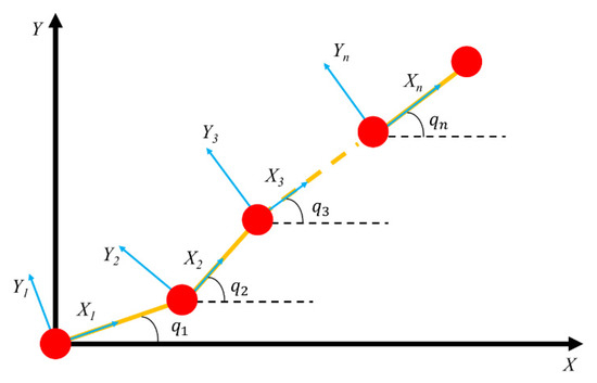
Figure 1. A sketch of a n-degree-of-freedom (n-DOF) robotic arm.

The dashed lines represent the initial positions of the robotic arm, with $q_1,q_2,...q_n$ indicating the joint rotation angles of the robotic arm.

Let $i=\mathrm{1,2},\dots ,n$, where $u_{i max}>0$ and $-u_{i min}<0$ specify the maximum and minimum limits of the torque, respectively. The control laws $u_i$ are designed with the known parameters $u_{i max}>0$ and $u_{i min}>0$; the functions $g_{ri}\left(u_i\right)$ and $g_{li}\left(u_i\right)$ are nonlinear and unknown with respect to $u_i$.

$$\ddot{q}=M^{-1}\left(q\right)\left[\tau \left(t\right)-C\left(q,\dot{q}\right)-G\left(q\right)\right]$$

(2)

The inertia matrix $M\left(q\right)$ possesses the properties of symmetry and positive definiteness. The matrix $\left(\dot{M}\left(q\right)-2C\left(q, \dot{q}\right)\right)$ demonstrates skew-symmetry.

2.1. Input Saturation Nonlinearity

In applications that require high precision and rapid responses, managing input saturation is a prevalent challenge. The primary role of input saturation nonlinearity in such systems is to regulate the extremities of control inputs, thereby ensuring both system stability and optimal control performance.

The saturation nonlinearity can be described as follows [35]:

$$\tau =D\left(u\right)+∆\tau$$

(3)

where the term $\tau$ denotes the approximation error, and the function $D\left(u\right)$ is given ${[D_1\left(u_1\right),D_2\left(u_2\right),\dots ,D_n(u_n\left)\right]}^T$.

$$D_i\left(u_i\right)={\displaystyle \frac{2{\overline{u}}_i}{\pi }}\mathrm{a}\mathrm{r}\mathrm{c}\mathrm{t}\mathrm{a}\mathrm{n}({\displaystyle \frac{\pi u_i}{2{\overline{u}}_i}})$$

(4)

where

$$\left\{\begin{array}{c}{\overline{u}}_i=u_{i max}. u_i\ge 0\\ {\overline{u}}_i=u_{i min}. u_i\le 0\end{array}\right.$$

(5)

By applying the mean value theorem, Equation (4) is formulated as follows:

$$\begin{gathered} D_i\left(u_i\right)={\displaystyle \frac{\partial D_i\left({\varrho }_i{u}_i\right)}{\partial u_i}}{u}_i+D_i\left(0\right) \\ ={\displaystyle \frac{u_i}{1+{\left(\frac{\pi {\varrho }_i{u}_i}{2{\overline{u}}_i}\right)}^2}} \\ =u_i-{\displaystyle \frac{{\left(\frac{\pi {\varrho }_i{u}_i}{2{\overline{u}}_i}\right)}^2}{1+{\left(\frac{\pi {\varrho }_i{u}_i}{2{\overline{u}}_i}\right)}^2}}{u}_i \end{gathered}$$

(6)

We initialize $D_i\left(0\right)$= 0 and assume that $0<{\varrho }_i<1$ for $i=1,\dots ,n$. The matrix $\zeta$ is defined as a diagonal matrix, with diagonal elements given by ${\left({\displaystyle \frac{\pi {\varrho }_i{u}_i}{2{\overline{u}}_i}}\right)}^2/(1+{({\displaystyle \frac{\pi {\varrho }_i{u}_i}{2{\overline{u}}_i}})}^2)$. It is determined that ${\left({\displaystyle \frac{\pi {\varrho }_i{u}_i}{2{\overline{u}}_i}}\right)}^2/(1+{({\displaystyle \frac{\pi {\varrho }_i{u}_i}{2{\overline{u}}_i}})}^2)$ is less than ${({\displaystyle \frac{\pi }{2}})}^2/(1+{({\displaystyle \frac{\pi }{2}})}^2)$ and thus less than 0.712. Consequently, it follows that the maximum eigenvalue of the matrix $\zeta$ does not exceed 0.712. Finally, the function $D\left(u\right)$ is reformulated as follows:

$$D\left(u\right)=u-\zeta u$$

(7)

2.2. Barrier Lyapunov Function

Within a system described by $\mathsf{\gamma }=D\left(\mathsf{\gamma }\right)$, when the system incorporates a continuous and strictly positive function $D\left(\mathsf{\gamma }\right)$, defined on an open set $\mathsf{\Omega }$, the function $V\left(\mathsf{\gamma }\right)$ is characterized as differentiable, with its first derivatives maintaining continuity throughout the domain $\mathsf{\Omega }$. A notable feature of $V\left(\mathsf{\gamma }\right)$ is its asymptotic behavior: it diverges to infinity as $\mathsf{\gamma }$ nears the periphery of $\mathsf{\Omega }$. Further, for any positive time $\mathrm{t}$ and any initial condition within $\mathsf{\Omega }$, specifically $\mathsf{\gamma }\left(0\right)$, the function $V\left(\mathsf{\gamma }\right)$, adheres to a strict upper bound, denoted by $\overline{V}$. This ensures that $V\left(\mathsf{\gamma }\right)$ remains strictly positive and does not exceed $\overline{V}$, thereby establishing $\overline{V}>V\left(\mathsf{\gamma }\right)>0$ across the domain.

To facilitate this, the adoption of the following RBF is warranted:

$$E={\displaystyle \frac{1}{2}}\mathrm{l}\mathrm{n}{\displaystyle \frac{a^2}{a^2-{\mathsf{\gamma }}^2}}$$

(8)

where the parameters dictate that $a$ must be greater than zero, with $\mathsf{\gamma }$ confined within the range of −a to a. Additionally, as the magnitude of $\mathsf{\gamma }$ approaches $a$, $\mathrm{E}$ grows infinitely large.

2.3. Radial Basis Function Neural Network

Neural networks are highly adept at modeling diverse nonlinear functions, as evidenced in references [9,32,33,34]. Their streamlined learning protocols enhance computational efficiency, making them ideal for addressing the uncertainties discussed in this study. In neural network models, the function approximation process involves mapping input data $H$ to the output $f_i\left(H\right)$, where $H$ is a feature vector from real-world applications and $H=[h_1,h_2,\dots ,h_q]\in O_H\complement R_q$. This mapping is achieved through the use of specific activation functions by each neuron in the network, typically Gaussian functions. The mathematical representation of this choice is as follows:

$$f_i\left(H\right)={\mathsf{\Phi }}_i^T{J}_i\left(H\right),\hspace{1em}i=\mathrm{1,2},\dots ,n$$

(9)

where ${\mathsf{\Phi }}_i$ denotes the weight vector corresponding to the i-th output, and $J_i\left(H\right)$ represents feature mapping based on the input $H$. This can be expressed as a collection of Gaussian functions:

$$J_i\left(H\right)=\left[j_1\left(H\right),j_2\left(H\right),\dots ,j_l\left(H\right)\right]$$

(10)

Each $j_n\left(H\right)$ is a Gaussian basis function, and can be defined as follows:

$$j_n\left(H\right)=exp\left[{\displaystyle \frac{-{\left(H-{\mu }_n\right)}^T\left(H-{\mu }_n\right)}{{{\eta }_n}^2}}\right],n=\mathrm{1,2},\dots ,l$$

(11)

To handle complex data effectively, the number of nodes l in the neural network must be sufficiently large. The centers of the Gaussian functions are denoted by ${\mu }_n$, and their widths ${\eta }_n$ determine the range of these functions. By adjusting the weights ${\mathsf{\Phi }}_i$ and the parameters of the basis functions, this configuration can effectively model the uncertainty of the system.

Working by approximation, the uncertain aspect of the system can be represented as follows [37]:

$$f_i\left(H\right)={\mathsf{\Phi }}_i^T{J}_i\left(H\right)+{\mathsf{\Delta }}_i\left(H\right),i=\mathrm{1,2},\dots ,n$$

(12)

where ${\mathsf{\Delta }}_i\left(H\right)$ denotes the bounded error, enabling the model to approximate nonlinear behaviors within an error constraint. ${\mathsf{\Phi }}_i$ is the ideal weight.

$${\mathsf{\Phi }}_{\mathrm{i}}=\underset{{\mathsf{\Phi }}_i\in R^l}{\mathrm{arg\; min}}\left\{\underset{H\in O_H}{\sup }\left|f_i\left(H\right)-{\mathsf{\Phi }}_i^T{J}_i\left(H\right)\right|\right\}$$

(13)

This targets the best weight vector ${\mathsf{\Phi }}_i$, which minimizes the maximum deviation between the actual function and the neural network approximation across all inputs, enhancing the model’s precision in uncertain environments.

2.4. Improved Sparrow Search Algorithm (ISSA)

The SSA is a nature-inspired optimization algorithm inspired by the foraging behavior and predator evasion tactics of sparrows [7]. In order to solve various optimization problems, this algorithm simulates the patterns of behavior exhibited by sparrow populations when searching for food, being vigilant, and escaping from predators. The sparrow population is typically divided into two main roles: leader sparrows (explorers) and followers. Leader sparrows primarily explore unknown areas to find resources, while followers change their positions based on the information provided by the leader sparrows [25].

Firstly, it is necessary to initialize the positions of the sparrow population. Each sparrow represents a potential solution. Sparrows update their positions either randomly or in a way that is partially guided by relevant information in order to simulate foraging. The formula is often expressed as follows:

$$x_i\left(t+1\right)=x_i\left(t\right)+r_1\times \left(x_{best}\left(t\right)-x_i\left(t\right)\right)+r_2\times \left(x_i\left(t\right)-x_{worst}\left(t\right)\right)$$

(14)

where $x_i\left(t\right)$ is the position of sparrow $\mathrm{i}$ at time $\mathrm{t}$, $x_{best}\left(t\right)$ and $x_{worst}\left(t\right)$ are the best and worst positions in the current population, respectively, and $r_1$ and $r_2$ are random numbers.

While searching for food, sparrows must also remain vigilant to avoid becoming prey. This is typically achieved through another position updating strategy, such as the following:

$$x_i\left(t+1\right)=x_i\left(t\right)+r_3\times sgn\left(r_4-0.5\right)\times \left(LB+r_5\times \left(UB-LB\right)\right)$$

(15)

where $r_3$, $r_4$, and $r_5$ are random numbers, $sgn$ is the sign function, and $LB$ and $UB$ are the lower and upper bounds of the solution space, respectively.

When sparrows perceive the threat of a predator, they rapidly change location to evade the threat. This process can be modeled with the following formula:

$$x_i\left(t+1\right)=x_{rand}\left(t\right)-r_6+\left|x_{rand}\left(t\right)-x_i\left(t\right)\right|$$

(16)

where $x_{rand}\left(t\right)$ is a randomly chosen sparrow’s position from the population, and $r_6$ is a random number.

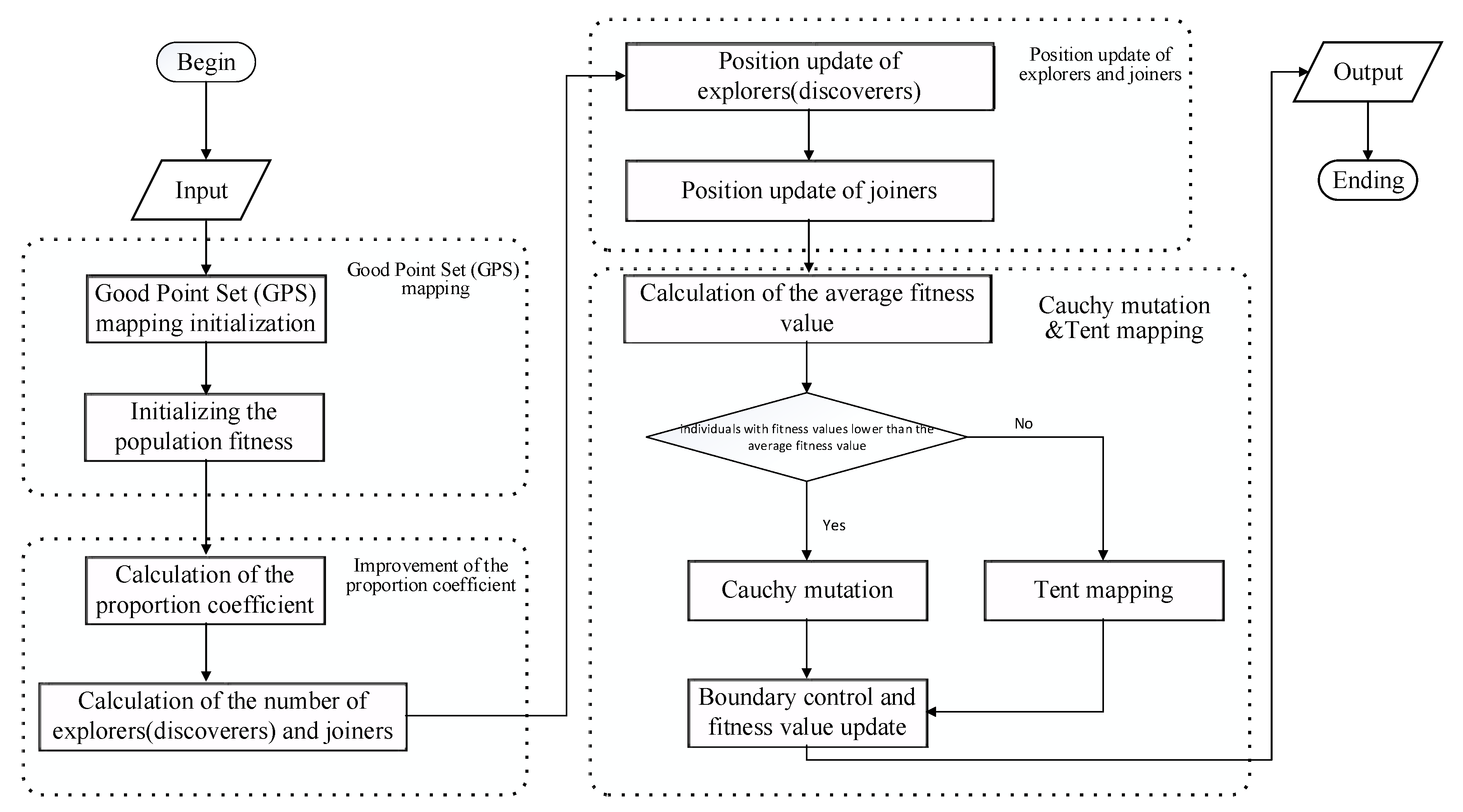
As shown in Figure 2, the improved sparrow search algorithm (ISSA) begins by accepting inputs, such as the population size, maximum iterations, and the lower and upper bounds of the search space. Initially, the population is generated through good point set (GPS) mapping, which enhances the diversity of the population and ensures better coverage of the search space. Following the initialization, the fitness of each individual in the population is calculated using the objective function, and the individuals are sorted based on their fitness values in order to identify the best and worst solutions. As the algorithm progresses, a proportion coefficient is calculated based on a warning threshold (ST) and a disturbance factor (k). This is used to dynamically adjust the balance between exploration and exploitation throughout the iterations. The next step involves calculating the number of explorers (discoverers) and joiners within the population. Explorers, responsible for finding new directions in the search space, update their positions using an improved formula or random perturbations, depending on the current fitness landscape and the global best solution. Joiners, on the other hand, update their positions relative to other individuals in the population, incorporating noise or differential vectors to refine their search. After updating positions, the average fitness of the population is calculated, serving as a criterion for determining which individuals undergo mutation-based operations. Individuals with fitness values below the population average are subjected to Cauchy mutation, introducing larger perturbations in order to facilitate exploration. Meanwhile, individuals with higher fitness values experience tent mapping, which finetunes their positions for exploitation. The algorithm incorporates boundary control to ensure that all individuals remain within the defined search space. This is followed by updates to the fitness values based on the new positions. This process iterates, with continuous updates to the global best solution, until either convergence is reached or the maximum number of iterations is completed, at which point the best position and fitness score are generated as the final outputs.

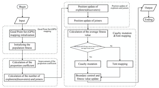
Figure 2. The workflow of ISSA.

Although the traditional sparrow search algorithm (SSA) has demonstrated a commendable performance in various optimization problems through its emulation of natural sparrow foraging and predator evasion behaviors, the algorithm encounters challenges when addressing some complex optimization scenarios. In high-dimensional and multimodal problems in particular, traditional SSA can sometimes become trapped in local optima, and its convergence speed may be suboptimal [28,29,30,31]. Moreover, balancing exploration and exploitation capabilities remains a key area for enhancement. To overcome these limitations, this research proposes an improved sparrow search algorithm (ISSA) that incorporates several key innovations to enhance the original framework:

(1)

The good point set (GPS) is a strategy for generating initial solution sets characterized by high uniformity and low correlation. It is suitable for use in global optimization problems. This strategy involves selecting the smallest prime number $p$ greater than $2N+3$, coupled with the use of the cosine function, to create a point set. The specific formula for generating points is as follows:

$$G_{ij}=i\times 2cos\left({\displaystyle \frac{2\pi \times j}{p}}\right) mod 1,i=\mathrm{1,2},\dots ,M;j=\mathrm{1,2},\dots ,N$$

(17)

where $i$ and $j$ represent the indices of the points and dimensions, respectively, M denotes the total number of points, and $N$ indicates the dimensions of the problem. Each point $G_{ij}$ is subsequently mapped to the actual search space by scaling linearly to the respective dimension’s upper $u{b}_j$ and lower bounds $l{b}_j$:

$$Positons={lb}_j+\left(u{b}_j-l{b}_j\right)\times G_{ij}$$

(18)

Thus, the good point set ensures the uniform distribution of the initial population in the parameter space, effectively enhancing the diversity of solutions and reducing clustering among them. This contributes to improving the global search capabilities and the efficiency of optimization algorithms.

(2)

By dynamically adjusting the proportion of discoverers and joiners, this improvement aims to balance exploration and exploitation capabilities. The proportional coefficient changes dynamically with the number of iterations, allowing for more explorers to investigate the solution space early in the search and increasing the number of joiners later on in order to refine potential solution areas already identified [27].

The calculation method for the proportional coefficient $\mathrm{r}$ is as follows:

$$\mathrm{r}=\mathrm{b}\times \left(\tan \left(-{\displaystyle \frac{\pi i}{4\times Ma{x}_{i}ter}}+{\displaystyle \frac{\pi }{4}}\right)\right)-\mathrm{k}\times \mathrm{r}\mathrm{a}\mathrm{n}\mathrm{d}$$

(19)

where $i$ is the current iteration number, $\mathrm{b}$ and $\mathrm{k}$ are coefficients, and $\mathrm{r}\mathrm{a}\mathrm{n}\mathrm{d}$ generates a random number within the [0, 1] interval. $Max\_iter$ indicates the maximum number of iterations.

(3)

This enhancement uses an exponential decay factor to adjust the position updates of explorers in order to optimize their efficiency when searching the solution space [25].

If ${\mathrm{X}}^{\left(i\right)}$ be the position of the j-th explorer at iteration i, the update formula is as follows:

$$X_j^{\left(i+1\right)}=X_j^{\left(i\right)}\times \left(2\times \mathrm{e}\mathrm{x}\mathrm{p}\left(-{\displaystyle \frac{4i}{{\left(\xi \times Ma{x}_{i}ter\right)}^2}}\right)\right)$$

(20)

where $\xi$ is a random number within the interval [0, 1].

(4)

This improvement increases population diversity by combining a tent map and Cauchy mutation, thereby enhancing the algorithm’s ability to avoid local optima and explore new areas [29,30,31]. Cauchy mutation is used when an individual’s fitness value is less than the average fitness value of the population. Tent mapping is used when an individual’s fitness value is greater than or equal to the average fitness value of the population.

Cauchy mutation is determined. If $X_j^{\left(i\right)}$ is the position of the j-th individual at iteration i, the position ${\tilde{X}}_j^{(i+1)}$ after Cauchy mutation is calculated as follows:

$${\tilde{X}}_j^{\left(i+1\right)}=X_j^{\left(i\right)}+\vartheta \times X_j^{\left(i\right)}$$

(21)

It is necessary to generate a Cauchy random number $\vartheta :$

$$\vartheta =tan\left(\left(rand\left(\mathrm{0,1}\right)-0.5\right)\times \pi \right)$$

(22)

where $rand (0,1)$ is a random number within the interval [0, 1].

Is $x_0$ is a random number in the interval [0, 1], the disturbance value tentV is computed as follows:

$$\mathrm{t}\mathrm{e}\mathrm{n}\mathrm{t}\mathrm{V}=\left\{\begin{array}{c}2x_0+{\displaystyle \frac{\varsigma }{pop}} if x_0<0.5\hfill \\ 2\left(1-x_0\right)+{\displaystyle \frac{\varsigma }{pop}} otherwise\hfill \end{array}\right.$$

(23)

Then, the position ${\tilde{X}}_j^{(i+1)}$ after tent mapping is as follows:

$${\tilde{X}}_j^{\left(i+1\right)}=X_j^{\left(i\right)}+tenV\times X_j^{\left(i\right)}$$

(24)

where $\varsigma$ is a random number within the interval [0, 1], and $pop$ is the population size.

2.5. Preliminaries

Lemma 1 [38].

This asserts that for any real numbers $a_1,a_2,\dots ,a_n$, and for $0\le x\le 1,$ the inequality ${(\left|a_1\right|+\cdots \left|a_n\right|)}^x\le {\left|a_1\right|}^x+\cdots +{\left|a_n\right|}^x$ is valid. This lemma is essential for bounding the cumulative errors in nonlinear control environments.

Lemma 2 [20].

The Cauchy–Schwarz inequality is formalized as ${\left({\sum }_{j=1}^n{x}_j\right)}^2\le n·{\sum }_{j=1}^n{x}_j^2$. It plays a critical role in assessing the stability and convergence properties of the system.

Lemma 3 [39].

The inequality $xy\le {\displaystyle \frac{{\mu }^a}{a}}{\left|x\right|}^a+{\displaystyle \frac{1}{b{\mu }^b}}{\left|y\right|}^b$for $x,y\in R$,$\mu >0$,$a>0$,$b>0$, and $(a-1)(b-1)=1$is a form of Young’s inequality, which is useful for controlling product terms in analysis.

Lemma 4 [40].

In Lemma 4, it is posited that $P$, an $n\times n$-dimensional real symmetric positive definite matrix, adheres to a crucial inequality for all $a\in R^n$. Specifically, the quadratic form $a^{T}Pa$ for any vector $a$ is bounded by ${\lambda }_{min}\left(P\right){‖a‖}^2$ and ${\lambda }_{max}\left(P\right){‖a‖}^2$, where ${\lambda }_{min}\left(P\right)$ and ${\lambda }_{max}\left(P\right)$ represent the minimum and maximum eigenvalues of $P,$ respectively. This lemma highlights essential properties of linear algebra and matrix theory, facilitating the estimation of the impact matrix operations have on vectors.

Lemma 5 [14].

It is necessary to assume that for a system $x\left(t\right)$, the origin is an equilibrium point, meaning the initial condition is $x\left(0\right)=x_0$, and the dynamics of the system are described by $\dot{x}\left(t\right)=f(t,x)$. If there exists a positive function $V\left(x\right)$ and constants $\Gamma ,\Psi >0$, with $0<q<1$ and $q>1$, the f is determined as follows:

$$\dot{V}\left(x\right)\le -\mathsf{\Gamma }{V}^p\left(x\right)-\mathsf{\Psi }{V}^q\left(x\right)$$

(25)

The origin point is stable, the convergence speed does not change with time, and the upper limit of the system’s stable time $T_d$ follows the following relationship:

$$T_d\le {\displaystyle \frac{1}{\mathsf{\Gamma }\left(p-1\right)}}+{\displaystyle \frac{1}{\mathsf{\Psi }\left(1-q\right)}}$$

(26)

Remark 1 [41].

There are various definitions for the settling time function $T_d$, and this article adopts an approach that is distinct from that used in previous research. By employing our definition, we demonstrate the practical efficacy and benefits of the fixed-time control strategy.

3. Fixed-Time Control Design and Lyapunov Function Proof Process

3.1. Fixed-Time Control Design

The error signal between the actual state and the desired trajectory is determined as follows:

$$e_1=q-q_d$$

(27)

The derivative of $e_1$ is given by the following:

$${\dot{e}}_1=e_2+\alpha -{\dot{q}}_d$$

(28)

The error signal between the actual velocity and the virtual control variable is determined as follows:

$$e_2=\dot{q}-\alpha$$

(29)

where $\alpha$ is the virtual control and $q_d$ is the desired trajectory. The barrier Lyapunov function (BLF) is formulated as follows:

$$V_1={\displaystyle \frac{1}{2}}\mathrm{l}\mathrm{n}{\displaystyle \frac{k_P^2}{k_P^2-{e_1}^T{e}_1}}$$

(30)

The selection of this function aims to ensure that the system state remains within the specified constraints by employing $k_P$ control. It also aims to achieve system stability through the regulation of the error $e_1$. The parameter $k_P>0$ serves to enforce the constraints on the system state.

$$k_P=a{e}^{-\epsilon t}+b$$

(31)

In this formula, $a$, $b$, and $\epsilon$ are real numbers that satisfy the conditions $a\ge 0$, $b\ge 0$,$\mathrm{and}\epsilon \ge 0$. These parameters are chosen and tuned based on the required error convergence trajectory.

Taking the time derivative of $V_1$ yields ${\dot{V}}_1$:

$$\begin{gathered} {\dot{V}}_1={\displaystyle \frac{{e_1}^T{\dot{e}}_1-\frac{{\dot{k}}_P}{k_P}{e_1}^T{e}_1}{k_P^2-{e_1}^T{e}_1}} \\ \hspace{1em}\hspace{1em}\hspace{1em}\hspace{1em}\hspace{1em} ={\displaystyle \frac{{e_1}^T\left({\mathrm{e}}_2+\alpha -{\dot{q}}_d\right)-\frac{{\dot{k}}_P}{k_P}{e_1}^T{e}_1}{k_P^2-{e_1}^T{e}_1}} \end{gathered}$$

(32)

α is designed as follows:

$$\begin{gathered} \alpha =-A_{11}{\displaystyle \frac{e_1\left(k_p^2-{e_1}^T{e}_1\right)}{{e_1}^T{e}_1}}{\left({\displaystyle \frac{1}{2}}\mathit{ln}\left({\displaystyle \frac{k_p^2}{k_p^2-{e_1}^T{e}_1}}\right)\right)}^{{\displaystyle \frac{1}{2}}}- \\ {A}_{12}{\displaystyle \frac{e_1\left(k_p^2-{e_1}^T{e}_1\right)}{{e_1}^T{e}_1}}{\left({\displaystyle \frac{1}{2}}\mathit{ln}\left({\displaystyle \frac{k_p^2}{k_p^2-{e_1}^T{e}_1}}\right)\right)}^2+{\dot{q}}_d-\left({\displaystyle \frac{1}{2}}+\epsilon \right)e_1 \end{gathered}$$

(33)

In this context, $A_{11}>0$ and $A_{12}>0$ are design constants.

Given that ${e_1}^T{e}_1\le {\displaystyle \frac{1}{2}}{e_1}^T{e}_1+{\displaystyle \frac{1}{2}}{e_2}^T{e}_2$ and that we aim for the system output to remain within the predetermined range where $\left|{\displaystyle \frac{\dot{k_P}}{k_P}}\right|\le \epsilon$, by substituting (33) into (32), we obtain the following:

$$\begin{gathered} {\dot{\mathrm{V}}}_1\le {\displaystyle \frac{\frac{1}{2}{{\mathrm{e}}_2}^T{\mathrm{e}}_2}{k_P^2-{e_1}^T{e}_1}}-A_{11}{\left({\displaystyle \frac{1}{2}}\ln \left({\displaystyle \frac{k_p^2}{k_p^2-{e_1}^T{e}_1}}\right)\right)}^{{\displaystyle \frac{1}{2}}}-A_{12}{\left({\displaystyle \frac{1}{2}}\ln \left({\displaystyle \frac{k_p^2}{k_p^2-{e_1}^T{e}_1}}\right)\right)}^2 \\ \le {\displaystyle \frac{\frac{1}{2}{e_2}^T{e}_2}{k_P^2-{e_1}^T{e}_1}}-A_{11}\sqrt{V_1}-A_{12}{V_1}^2 \end{gathered}$$

(34)

The fixed-time control signal $\mathsf{\beta }$ is structured as follows:

$$\mathsf{\beta }={\mathsf{\beta }}^a+{\mathsf{\beta }}^b$$

(35)

Here, ${\mathsf{\beta }}^a$ and ${\mathsf{\beta }}^b,$ based on errors $e_1$ and $e_2$, are defined as follows:

$$\begin{gathered} {\mathsf{\beta }}^a=-{\displaystyle \frac{1}{2}}\left({\displaystyle \frac{1}{k_P^2-{e_1}^T{e}_1}}+1\right)e_2+{\widehat{\mathsf{\Phi }}}^{T}J\left(H\right)-A_{21}{\displaystyle \frac{e_2}{{e_2}^T{e}_2}}{\left({\displaystyle \frac{1}{2}}{e_2}^T{e}_2\right)}^{{\displaystyle \frac{1}{2}}} \\ -A_{22}{\left({\displaystyle \frac{1}{2}}\right)}^2{e}_2{e_2}^T{e}_2 \end{gathered}$$

(36)

$${\mathsf{\beta }}^b=-{\displaystyle \frac{‖{\mathsf{\beta }}^a‖e_2}{‖e_2‖\left(1-{\lambda }_{max}\left(\zeta \right)\right)}}$$

(37)

Key parameters include design gains $A_{21}$ and $A_{22}$, both of which are positive values, and ${\lambda }_{max}\left(\zeta \right)$ denotes the maximum eigenvalue of the matrix $\zeta .$ It is recommended that the latter not exceed 0.712. $\widehat{\mathsf{\Phi }}$ denotes the estimation of $\mathsf{\Phi }$.

To address the uncertainties in dynamics, we employ a radial basis function (RBF) neural network to help reduce system errors.

$${\mathsf{\Phi }}^{T}J\left(H\right)=M\left(q\right)\dot{\alpha }+C\left(q,\dot{q}\right)\alpha -G\left(q\right)-\mathsf{\Delta }\tau -\sigma \left(H\right)$$

(38)

where $\mathsf{\Phi }$ symbolizes the network’s optimal weight vector, and $H$ encompasses the input parameters, including position $q$ and velocity $\dot{q}$. The function $J\left(H\right)$ represents the basis function deployed within the network, while $\sigma \left(H\right)$ indicates the bounded approximation error, with $\sigma >0$ signifying the bound.

To ensure the convergence of the speed error, we design $V_2$ as follows:

$$V_2={\displaystyle \frac{1}{2}}{e_2}^{T}M\left(q\right)e_2$$

(39)

The result of differentiating $V_2$ obtained through Appendix A is as follows:

$${\dot{V}}_2\le -{\displaystyle \frac{\frac{1}{2}{e_2}^T{e}_2}{k_P^2-{e_1}^T{e}_1}}-{\displaystyle \frac{A_{21}}{\sqrt{{\mathsf{\lambda }}_{\mathrm{m}\mathrm{a}\mathrm{x}}\left(M\left(q\right)\right)}}}\sqrt{V_2}-{\displaystyle \frac{A_{22}}{{\mathsf{\lambda }}_{\mathrm{m}\mathrm{a}\mathrm{x}}^2\left(M\left(q\right)\right)}}{V_2}^2+{e_2}^{\mathrm{T}}{\tilde{\mathsf{\Phi }}}^{\mathrm{T}}J\left(H\right)+{\displaystyle \frac{1}{2}}{\overline{\mathsf{\sigma }}}^2$$

(40)

$\tilde{\mathsf{\Phi }}$ represents the weight of the difference between the actual state and the desired value, and we design a rule for use updating the neural network as follows:

$${\dot{\widehat{\mathsf{\Phi }}}}_i=-{\mathsf{\Lambda }}_i\left[J\left(H\right)e_{2i}+{\widehat{\mathsf{\Phi }}}_i{\widehat{\mathsf{\Phi }}}_i^T{\widehat{\mathsf{\Phi }}}_i+{\epsilon }_i{\widehat{\mathsf{\Phi }}}_i\right]$$

(41)

where ${\mathsf{\Lambda }}_i$ signifies the constant matrices, and ${\epsilon }_i$ denotes the constants employed to augment the robustness of the system. $i=\mathrm{1,2},\dots ,\mathrm{n}$.

We designed $V_3$ to handle system uncertainties and external disturbances, ensuring to improve the robustness of the system.

$$V_3={\displaystyle \frac{1}{2}}\sum _{i=1}^n{\tilde{\mathsf{\Phi }}}_i^T{\mathsf{\Lambda }}_i^{-1}{\tilde{\mathsf{\Phi }}}_i$$

(42)

The result of differentiating $V_3$, obtained from Appendix B, is as follows:

$${\dot{V}}_3\le -A_{31}\sqrt{V_3}-{\displaystyle \frac{A_{32}}{n}}{V}_3^2-\sum _{i=1}^{\mathrm{n}}{\tilde{\mathsf{\Phi }}}_i^T{J}_i\left(H\right)e_{2i}+B_1$$

(43)

where

$$A_{31}=min\left\{{\displaystyle \frac{\sqrt{2}\left(2{‖{\mathsf{\Phi }}_i‖}^2+{\epsilon }_i\right)}{\sqrt{{\lambda }_{max}\left({\mathsf{\Lambda }}_i^{-1}\right)}}},i=\mathrm{1,2},...,\mathrm{n}\right\}$$

(44)

$$A_{32}=min\left\{{\displaystyle \frac{4\left(1-\frac{9}{4}{K}_{1i}^{\frac{4}{3}}-\frac{1}{4K_{2i}^4}\right)}{{\left({\lambda }_{max}\left({\mathsf{\Lambda }}_i^{-1}\right)\right)}^2}},i=\mathrm{1,2},...,\mathrm{n}\right\}$$

(45)

$$B_1=\sum _{i=1}^{\mathrm{n}}\left(\left({\displaystyle \frac{3}{4K_{1i}^4}}+{\displaystyle \frac{3}{4}}{K}_{2i}^{{\displaystyle \frac{4}{3}}}\right){‖{\mathsf{\Phi }}_i‖}^4+\left(1+{\displaystyle \frac{{\epsilon }_i}{2}}\right){‖{\mathsf{\Phi }}_i‖}^2+{\displaystyle \frac{{\epsilon }_i}{2}}\right)$$

(46)

where $K_{1i}>0$ and $K_{2i}>0$ are chosen such that $1>{\displaystyle \frac{9}{4}}{K}_{1i}^{{\displaystyle \frac{4}{3}}}+{\displaystyle \frac{1}{4K_{2i}^4}}$.

3.2. Lyapunov Function Proof

To demonstrate that $e_1$,$e_2$, and $\mathsf{\Phi }$ converge to distinct sets within the convergence time $T_D$, we derive the following Lyapunov equation based on the preceding discussion:

$$V=V_1+V_2+V_3$$

(47)

Deriving the derivative of the above equation yields the following:

$$\dot{V}\le -A_{11}\sqrt{V_1}-{\displaystyle \frac{A_{21}}{\sqrt{{\lambda }_{\mathrm{m}\mathrm{a}\mathrm{x}}\left(M\left(q\right)\right)}}}\sqrt{V_2}-A_{31}\sqrt{V_3}-A_{12}{V_1}^2-{\displaystyle \frac{A_{22}}{{{\lambda }_{\mathrm{m}\mathrm{a}\mathrm{x}}}^2\left(M\left(q\right)\right)}}{V}_2^2+{\displaystyle \frac{A_{32}}{n}}{V_3}^2+B$$

(48)

where

$$B=B_1+{\displaystyle \frac{1}{2}}{\overline{\sigma }}^2$$

(49)

Using Lemma 2 and Equation (48), we obtain the following:

$$\dot{V}\le -{\delta }_1\sqrt{V}-{\displaystyle \frac{{\delta }_2{V}^2}{3}}+B$$

(50)

where ${\delta }_1$ and ${\delta }_2$ have the following definitions:

$${\delta }_1=\mathrm{m}\mathrm{i}\mathrm{n}\left\{A_{11},{\displaystyle \frac{A_{21}}{\sqrt{{\lambda }_{\mathrm{m}\mathrm{a}\mathrm{x}}\left(M\left(q\right)\right)}}},A_{31}\right\}$$

(51)

$${\delta }_2=\mathrm{m}\mathrm{i}\mathrm{n}\left\{A_{21},{\displaystyle \frac{A_{22}}{\sqrt{{{\lambda }_{\mathrm{m}\mathrm{a}\mathrm{x}}}^2\left(M\left(q\right)\right)}}},{{\displaystyle \frac{1}{n}}A}_{32}\right\}$$

(52)

To ensure that $e_1$, $e_2$, and $\mathsf{\Phi }$ converge within the corresponding compact sets, and to allow $\mathrm{V}$ to converge within a specific interval, we eliminate the term B from (50), and set $V^2>{\displaystyle \frac{3B}{{\delta }_2}}$, which allows the system $V$ to eventually converge to the set $\{\mathrm{V}|0<\mathrm{V}<{({\displaystyle \frac{3B}{{\delta }_2}})}^{{\displaystyle \frac{1}{2}}}\}$. Furthermore, we design a constant $\mathsf{\Psi }$ within the interval from 0 to 1, which ensures that $B\le {\displaystyle \frac{\mathsf{\Psi }{\delta }_2}{3}}{V}^2$. Therefore, Equation (50) can be rephrased as follows:

$$\dot{V}\le -{\delta }_1\sqrt{V}-\left(1-\mathsf{\Psi }\right){\displaystyle \frac{{\delta }_2{V}^2}{3}}$$

(53)

Let $T_D$ represent the duration required for the system to reach a converged state within a fixed time period. According to Lemma 5, $T_D$ is designed as follows:

$$T_D\le {\displaystyle \frac{2}{{\delta }_1}}+{\displaystyle \frac{3}{\left(1-\mathsf{\Psi }\right){\delta }_2}}$$

(54)

Within a time ${\mathrm{T}}_{\mathrm{D}}$, $e1$, $e2$, and $\mathsf{\Phi }$ will each converge towards ${\mathsf{O}}_{e1},{\mathsf{O}}_{e2},{\mathsf{O}}_{\mathsf{\Phi }},$ respectively. These are designed as follows:

$${\mathsf{O}}_{{\mathrm{e}}_1}=\left\{{\mathrm{e}}_1\in R^n|‖{\mathrm{e}}_1‖\le k_p\sqrt{1-{\displaystyle \frac{1}{e^Y}}}\right\}$$

(55)

$${\mathsf{O}}_{{\mathrm{e}}_2}=\left\{{\mathrm{e}}_2\in R^n|‖{\mathrm{e}}_2‖\le \sqrt{{\displaystyle \frac{Y}{{\lambda }_{\mathrm{m}\mathrm{i}\mathrm{n}}\left(M\left(q\right)\right)}}}\right\}$$

(56)

$${\mathsf{O}}_{\tilde{\mathsf{\Phi }}}=\left\{\tilde{\mathsf{\Phi }}=[{\tilde{\mathsf{\Phi }}}_1,{\tilde{\mathsf{\Phi }}}_2,...,{\tilde{\mathsf{\Phi }}}_n]\in R^{l\times n}|‖\tilde{\mathsf{\Phi }}‖\le \sqrt{{\displaystyle \frac{Y}{{\lambda }_{\mathrm{m}\mathrm{i}\mathrm{n}}\left({\mathsf{\Lambda }}_i^{-1}\right)}}},i=\mathrm{1,2},...n\right\}$$

(57)

With

$$Y=2\sqrt{{\displaystyle \frac{3B}{{\delta }_2\mathsf{\Psi }}}}$$

(58)

4. Simulation

4.1. Simulation on ISSA Performance

In the simulation tests, eight standard benchmark functions (F1 to F8) were utilized to evaluate the performance of the ISSA. These functions are designed to test different aspects of the algorithm to ensure its efficiency, accuracy, and robustness. Among them, F1, F2, and F4 are unimodal functions, which are primarily used to test the convergence speed and efficiency of optimization algorithms. They help us to understand the algorithm’s performance as it approaches the optimal solution, as well as the algorithm’s speed and stability. On the other hand, F3, F5, F6, F7, and F8 are multimodal functions, which contain multiple local optima within their domains. This complexity makes it more challenging to locate the global optimum. Therefore, multimodal functions are employed to test the global search capabilities of optimization algorithms, specifically assessing whether the algorithm can effectively escape local optimal values and ultimately locate the global optimum.

In the simulation, we utilized six different optimization algorithms, namely the sparrow search algorithm (SSA), the improved sparrow search algorithm (ISSA), particle swarm optimization (PSO), chimpanzee optimization algorithm (Chimp), the grey wolf optimizer (GWO), and the whale optimization algorithm (WOA). The parameters for the algorithms were set as follows: the maximum number of iterations was set to 500, and the population size was set to 40. For the SSA and ISSA algorithms, the warning value was set to 0.6, the proportion of explorers was 0.7, and the proportion of sparrows aware of the danger was 0.3. In the PSO algorithm, the inertia factor was 0.9, and the learning factor was 2. In Chimp, the exploitation factor was 2. For the GWO and WOA methods, the dynamic adjustment parameter initial value was set to 2. Each function was run independently 10 times. The average value, optimal value, and worst value were recorded for the SSA, ISSA, PSO, GWO, Chimp, and WOA techniques.

The simulations were performed using MATLAB R2021a on a system running Windows 10 (64-bit) with an 11th Gen Intel (R) Core (TM) i5-11400F (Intel, Santa Clara, CA, USA) processor at 2.60 GHz.

Table 1, as regards F7, $u$ represents the penalty function, defined as $u=k·({(x-a)}^m·1_{x>a}+{(-x-a)}^m·1_{x<-a})$, where k = 100, a = 5, and m = 4. Here, $1_{x>a}$ is an indicator function that takes the value 1 if x > a and 0 otherwise, and $1_{x<-a}$ is another indicator function that takes the value 1 if $x<-a$ and 0 otherwise.

Table 1. Parameters of standard test functions.

Function Number	Test Functions	Domain	Theoretical Value
F1	$\mathbf{F}\mathbf{1}\left(\mathbf{x}\right)={\sum }_{\mathit{i}=\mathbf{1}}^{\mathbf{30}}{\mathit{x}}_{\mathit{i}}^{\mathbf{2}}$	[−100, 100]	0
F2	$\mathbf{F}\mathbf{2}\left(\mathbf{x}\right)={\sum }_{\mathit{i}=\mathbf{1}}^{\mathbf{30}}\left|{\mathit{x}}_{\mathit{i}}\right|+{\prod }_{\mathit{i}=\mathbf{1}}^{\mathbf{30}}\left|{\mathit{x}}_{\mathit{i}}\right|$	[−10, 10]	0
F3	$\mathbf{F}\mathbf{3}\left(\mathbf{x}\right)=\mathbf{1}-\mathbf{c}\mathbf{o}\mathbf{s}\left(\sqrt{{\sum }_{\mathit{i}=\mathbf{1}}^{\mathbf{30}}{\mathit{x}}_{\mathit{i}}^{\mathbf{2}}}\right)$	[−10, 10]	0
F4	$\mathbf{F}\mathbf{4}\left(\mathbf{x}\right)={\mathbf{m}\mathbf{a}\mathbf{x}}_{\mathit{i}}\left(\left|{\mathit{x}}_{\mathit{i}}\right|\right)$	[−100, 100]	0
F5	$\mathbf{F}\mathbf{5}\left(\mathbf{x}\right)={\sum }_{\mathit{i}=\mathbf{1}}^{\mathbf{30}}{\mathit{x}}_{\mathit{i}}^{\mathbf{2}}+{\left({\sum }_{\mathit{i}=\mathbf{1}}^{\mathbf{30}}{\displaystyle \frac{\mathbf{1}}{\mathbf{2}}}\mathit{i}{\mathit{x}}_{\mathit{i}}\right)}^{\mathbf{2}}+{\left({\sum }_{\mathit{i}=\mathbf{1}}^{\mathbf{30}}{\displaystyle \frac{\mathbf{1}}{\mathbf{2}}}\mathit{i}{\mathit{x}}_{\mathit{i}}\right)}^{\mathbf{4}}$	[−5, 10]	0
F6	$\mathbf{F}\mathbf{6}\left(\mathbf{x}\right)=-\mathbf{20}\mathbf{exp}\left(-\mathbf{0.2}\sqrt{{\displaystyle \frac{\mathbf{1}}{\mathbf{30}}}{\sum }_{\mathit{i}=\mathbf{1}}^{\mathbf{30}}{\mathit{x}}_{\mathit{i}}^{\mathbf{2}}}\right)-\mathbf{exp}\left({\displaystyle \frac{\mathbf{1}}{\mathbf{30}}}{\sum }_{\mathit{i}=\mathbf{1}}^{\mathbf{30}}\mathbf{cos}\left(\mathbf{2}\mathit{\pi }{\mathit{x}}_{\mathit{i}}\right)\right)+\mathbf{20}+\mathbf{e}$	[−32, 32]	0
F7	$$\begin{gathered} \mathbf{F}\mathbf{7}\left(\mathbf{x}\right)=\mathbf{0.1}\left[{\mathbf{s}\mathbf{i}\mathbf{n}}^{\mathbf{2}}\left(\mathbf{3}\mathit{\pi }{\mathit{x}}_{\mathbf{1}}\right) \\ \hspace{1em}\hspace{1em}\hspace{1em}\hspace{1em}\hspace{1em}\hspace{1em}+{\sum }_{\mathit{i}=\mathbf{1}}^{\mathbf{30}-\mathbf{1}}{\left({\mathit{x}}_{\mathit{i}}-\mathbf{1}\right)}^{\mathbf{2}}\left(\mathbf{1}+{\mathbf{sin}}^{\mathbf{2}}\left(\mathbf{3}\mathit{\pi }{\mathit{x}}_{\mathit{i}+\mathbf{1}}\right)\right) \\ \hspace{1em}\hspace{1em}\hspace{1em}\hspace{1em}\hspace{1em}\hspace{1em}+{\left({\mathit{x}}_{\mathbf{30}}-\mathbf{1}\right)}^{\mathbf{2}}\left(\mathbf{1}+{\mathbf{sin}}^{\mathbf{2}}\left(\mathbf{2}\mathit{\pi }{\mathit{x}}_{\mathbf{30}}\right)\right)\right]+{\sum }_{\mathit{i}=\mathbf{1}}^{\mathbf{30}}\mathit{u} \end{gathered}$$	[−50, 50]	0
F8	$\mathbf{F}\mathbf{8}\left(\mathbf{x}\right)={\sum }_{\mathit{i}=\mathbf{1}}^{\mathbf{11}}{({\mathit{c}}_{\mathit{i}}-{\displaystyle \frac{{\mathit{x}}_{\mathbf{1}}({\mathit{d}}_{\mathit{i}}^{\mathbf{2}}+{\mathit{x}}_{\mathbf{2}}{\mathit{d}}_{\mathit{i}})}{{\mathit{d}}_{\mathit{i}}^{\mathbf{2}}+{\mathit{x}}_{\mathbf{3}}{\mathit{d}}_{\mathit{i}}+{\mathit{x}}_{\mathbf{4}}}})}^{\mathbf{2}}$	[−5, 5]	0.000309

In F8, let $c_i=[0.1957,0.1947,0.1735,0.16,0.0844,0.0627,0.0456,0.3424,0.323,0.235,0.246]$ and $d_i=\left[{\displaystyle \frac{1}{0.25}},{\displaystyle \frac{1}{0.5}},1,{\displaystyle \frac{1}{2}},{\displaystyle \frac{1}{4}},{\displaystyle \frac{1}{6}},{\displaystyle \frac{1}{8}},{\displaystyle \frac{1}{10}},{\displaystyle \frac{1}{12}},{\displaystyle \frac{1}{14}},{\displaystyle \frac{1}{16}}\right]$ for $i=1,2,...,11$.

Table 2 presents the experimental results for six different algorithms across various functions. To illustrate the optimization performance of the algorithms, Figure 3 displays the iteration curves for each function.

Table 2. Experimental results for six different optimization algorithms.

Test Functions	Algorithm	Best Value	Worst Value	Average Value
F1	SSA	0.0000 × 100	4.0130 × 10−267	4.0130 × 10−268
	ISSA	0.0000 × 100	0.0000 × 100	0.0000 × 100
	PSO	6.3177 × 10−1	2.5751 × 100	1.6997 × 100
	Chimp	7.2228 × 10−10	5.0203 × 10−7	8.2238 × 10−8
	GWO	4.4064 × 10−32	2.8157 × 10−30	6.5511 × 10−31
	WOA	1.4104 × 10−89	6.9762 × 10−79	6.9780 × 10−80
F2	SSA	0.0000 × 100	1.0519 × 10−103	1.0519 × 10−104
	ISSA	0.0000 × 100	0.0000 × 100	0.0000 × 100
	PSO	2.4067 × 100	4.9044 × 100	3.8305 × 100
	Chimp	2.9009 × 10−7	1.9247 × 10−5	5.7236 × 10−6
	GWO	1.5962 × 10−19	2.7536 × 10−18	1.3757 × 10−18
	WOA	2.3018 × 10−59	6.1251 × 10−53	6.9522 × 10−54
F3	SSA	0.0000 × 100	0.0000 × 100	0.0000 × 100
	ISSA	0.0000 × 100	0.0000 × 100	0.0000 × 100
	PSO	0.0000 × 100	1.3654 × 10−10	1.4841 × 10−11
	Chimp	3.2463 × 10−10	−1.1122 × 10−7	2.3298 × 10−8
	GWO	8.4082 × 10−10	1.9413 × 10−7	3.1146 × 10−8
	WOA	0.0000 × 100	1.2829 × 10−12	1.4072 × 10−13
F4	SSA	0.0000 × 100	4.2410 × 10−252	4.2410 × 10−253
	ISSA	0.0000 × 100	0.0000 × 100	0.0000 × 100
	PSO	1.4490 × 100	2.0563 × 100	1.6774 × 100
	Chimp	2.2011 × 10−2	6.0196 × 10−1	2.0611 × 10−1
	GWO	1.7687 × 10−8	2.1929 × 10−7	5.8221 × 10−8
	WOA	9.8640 × 10−2	8.5463 × 101	4.5762 × 101
F5	SSA	0.0000 × 100	3.0119 × 10−124	3.0119 × 10−125
	ISSA	0.0000 × 100	0.0000 × 100	0.0000 × 100
	PSO	6.2717 × 101	1.7519 × 102	1.2573 × 102
	Chimp	1.7803 × 100	2.2152 × 101	9.1301 × 100
	GWO	1.4177 × 10−11	4.5254 × 10−9	1.0949 × 10−9
	WOA	5.0206 × 102	2.9749 × 102	4.3256 × 102
F6	SSA	8.8818 × 10−16	8.8818 × 10−16	8.8818 × 10−16
	ISSA	8.8818 × 10−16	8.8818 × 10−16	8.8818 × 10−16
	PSO	1.0527 × 100	3.0465 × 100	2.2359 × 100
	Chimp	1.9961 × 101	1.9964 × 101	1.9963 × 101
	GWO	5.0626 × 10−14	7.5495 × 10−14	6.1995 × 10−14
	WOA	8.8818 × 10−16	7.9936 × 10−15	4.0856 × 10−15
F7	SSA	1.4742 × 10−6	1.4673 × 10−2	5.0658 × 10−3
	ISSA	5.7401 × 10−5	2.4232 × 10−2	3.3781 × 10−3
	PSO	2.1128 × 10−1	9.0880 × 10−1	4.6949 × 10−1
	Chimp	2.6782 × 100	2.9905 × 100	2.8295 × 100
	GWO	3.0732 × 10−1	7.2904 × 10−1	5.0930 × 10−1
	WOA	1.2416 × 10−1	9.4357 × 10−1	3.1349 × 10−1
F8	SSA	3.1419 × 10−4	1.2254 × 10−3	5.2091 × 10−4
	ISSA	3.0750 × 10−4	3.6394 × 10−4	3.1646 × 10−4
	PSO	7.9768 × 10−4	9.9879 × 10−4	9.1620 × 10−4
	Chimp	1.2354 × 10−3	1.3394 × 10−3	1.2804 × 10−3
	GWO	3.0755 × 10−4	2.0363 × 10−2	4.4465 × 10−3
	WOA	3.1812 × 10−4	6.9223 × 10−4	4.9395 × 10−4

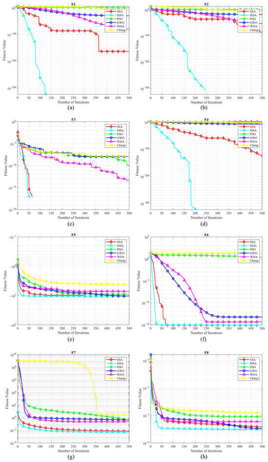
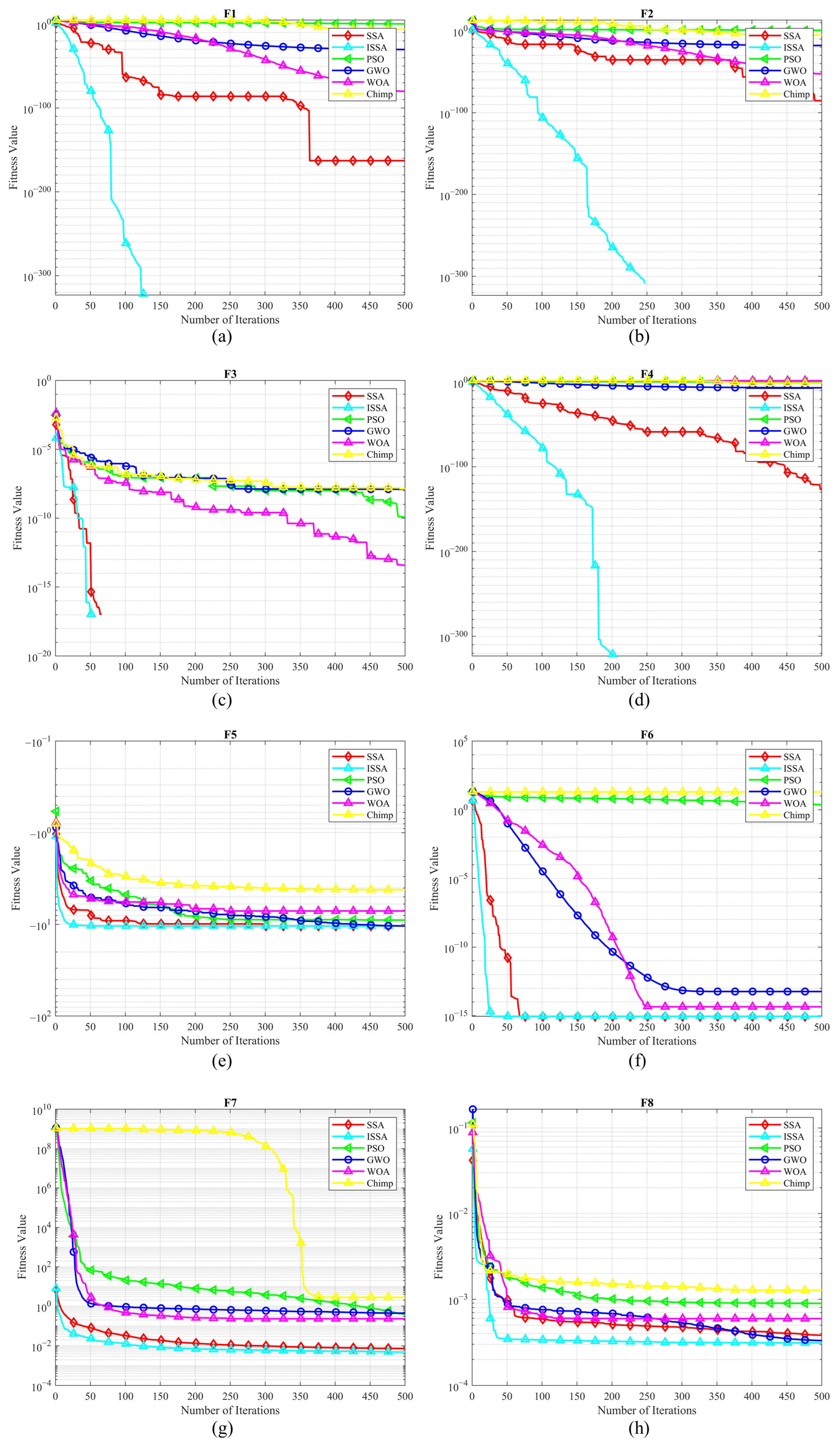
Figure 3. Iteration curves for functions F1 to F8. (a) Iteration curve for F1. (b) Iteration curve for F2. (c) Iteration curve for F3. (d) Iteration curve for F4. (e) Iteration curve for F5. (f) Iteration curve for F6. (g) Iteration curve for F7. (h) Iteration curve for F8.

Figure 3 shows the changes in the fitness values of six optimization algorithms when one is finding the optimal values of eight test functions with increasing iterations. It can be seen from the diagrams that ISSA demonstrates a superior optimization capability in all test functions, with faster convergence and higher solution precision. For instance, in unimodal functions F1, F2, and F4, ISSA’s convergence rate is significantly higher than that of other algorithms, with values matching the theoretical ones, thus showing the highest solution precision. Compared to SSA, which has the second highest solution precision, ISSA’s precision is greater by more than 100 orders of magnitude. In multimodal functions F3, F5, F6, F7, and F8, ISSA performs best when comparing optimal, worst, and average values. In F3, the ISSA algorithm demonstrates a rapid initial decline, stabilizing after approximately 50 iterations, indicating an exceptionally fast convergence rate. In comparison, both the SSA and PSO algorithms also stabilize after around 50 iterations, but their convergence speed and precision values are slightly inferior to those of ISSA. In F5, the final convergence value of ISSA is the lowest among all the algorithms, indicating that there is a more optimal solution. The final convergence values of PSO and GWO are slightly higher than those of ISSA and SSA, but they are still at a relatively good level. WOA and Chimp exhibit significant fluctuations throughout the entire iteration process, resulting in lower final precision values. In F6, neither Chimp nor PSO found the ideal solution, with ISSA showing more than 15 times greater precision. In F6, ISSA and SSA have the same average value of 8.8818 × 10⁻¹⁶, but ISSA converges faster. In F7 and F8, the ISSA solution still exhibits the highest accuracy. Notably, in F7, the Chimp algorithm does not produce an exact solution. The iteration curves from Figure 3 indicate that the ISSA algorithm can prevent a search from becoming trapped in local optima, thus enhancing the solution precision and search capability of the algorithm.

4.2. Two-DOF Robotic Arm Simulation

In this section, the proposed control scheme is applied to a two-degree-of-freedom robotic arm simulation platform to verify its effectiveness. Specific simulation platform parameters are shown in Table 3. The simulations were carried out in two parts, using the proposed fixed-time control combined with an improved sparrow search algorithm. To validate the robustness of the algorithm, we compared it with traditional PD control.

Table 3. Parameters of the two-DOF robotic arm.

Parameters	Meaning	Value	Unit
${\mathit{M}}_{\mathbf{1}}$	Mass of link 1	3.64	kg
${\mathit{M}}_{\mathbf{2}}$	Mass of link 2	0.42	kg
${\mathbf{L}}_{\mathbf{1}}$	Length of link 1	0.301	m
${\mathbf{L}}_{\mathbf{2}}$	Length of link 2	0.094	m
${\mathbf{I}}_{\mathbf{1}}$	Inertia of link 1	${\mathbf{L}}_{\mathit{X}\mathit{X}}=\mathbf{0.0437}$; ${\mathbf{L}}_{\mathit{X}\mathit{Y}}=\mathbf{0.0003}; {\mathbf{L}}_{\mathit{X}\mathit{Z}}=\mathbf{0.0000}$	$\mathbf{k}\mathbf{g}/{\mathbf{m}}^{\mathbf{2}}$
		${\mathbf{L}}_{\mathit{Y}\mathit{X}}=\mathbf{0.0003}; {\mathbf{L}}_{\mathit{Y}\mathit{Y}}=\mathbf{0.0065}; {\mathbf{L}}_{\mathit{Y}\mathit{Z}}=\mathbf{0.0071}$
		${\mathbf{L}}_{\mathit{Z}\mathit{X}}=\mathbf{0.0000}; {\mathbf{L}}_{\mathit{Z}\mathit{Y}}=\mathbf{0.0071}; {\mathbf{L}}_{\mathit{Z}\mathit{Z}}=\mathbf{0.0071}$
${\mathbf{I}}_{\mathbf{2}}$	Inertia of link 2	${\mathbf{L}}_{\mathit{X}\mathit{X}}=\mathbf{0.0004}; {\mathbf{L}}_{\mathit{X}\mathit{Y}}=\mathbf{0.0000}; {\mathbf{L}}_{\mathit{X}\mathit{Z}}=\mathbf{0.0000}$	$\mathbf{k}\mathbf{g}/{\mathbf{m}}^{\mathbf{2}}$
		${\mathbf{L}}_{\mathit{Y}\mathit{X}}=\mathbf{0.0000}; {\mathbf{L}}_{\mathit{Y}\mathit{Y}}=\mathbf{0.0065}; {\mathbf{L}}_{\mathit{Y}\mathit{Z}}=\mathbf{0.0000}$
		${\mathbf{L}}_{\mathit{Z}\mathit{X}}=\mathbf{0.0000}; {\mathbf{L}}_{\mathit{Z}\mathit{Y}}=\mathbf{0.0000}; {\mathbf{L}}_{\mathit{Z}\mathit{Z}}=\mathbf{0.0010}$

The simulations were performed using MATLAB R2021a on a system running Windows 10 (64-bit) with an 11th Gen Intel (R) Core (TM) i5-11400F processor at 2.60 GHz.

The first part of the simulation was conducted without the sparrow search algorithm. In the second part, we presented the simulation results of the control scheme with the sparrow algorithm and compared them to those of the control without the sparrow search algorithm. To compare control performance, we chose the same desired signals, $q_{1d}$ and $q_{2d}$, as were utilized for 0.3 rad and 0.2 rad, respectively, and we set the same initial conditions as were used for $q=[0,0]$ and $\dot{q}=[0,0]$.

There are 5 nodes in the hidden layer of the neural network, with the activity centers of the hidden layer nodes set at [−1, −0.5, 0, 0.5, 1], and the variance of the basis function is 1. The control parameters are set to $A_{11}=0.1, A_{12}=0.01 , A_{21}=0.01 {, A}_{22}=0.001$, and $\zeta =0.7$, and the initial weight is ${\mathsf{\Phi }}_{ij}=0$, where $i=1, 2$ and $j=\mathrm{1,2},\dots , 5$. Since the desired trajectory is a square wave, the error suddenly changes when the signal jumps. Therefore, $k_P=10$ was chosen to control the amplitude of oscillation. Symmetric input saturation constraints were chosen with corresponding values of ${\tau }_{1max}=9$ Nm, ${\tau }_{1min}=-9$ Nm,${\tau }_{2max}=6$ Nm and ${\tau }_{2min}=-6$ Nm, ${\mathsf{\Lambda }}_i=10I_{5\times 5}$,${\epsilon }_i=0.0002$, and $i=1, 2$.

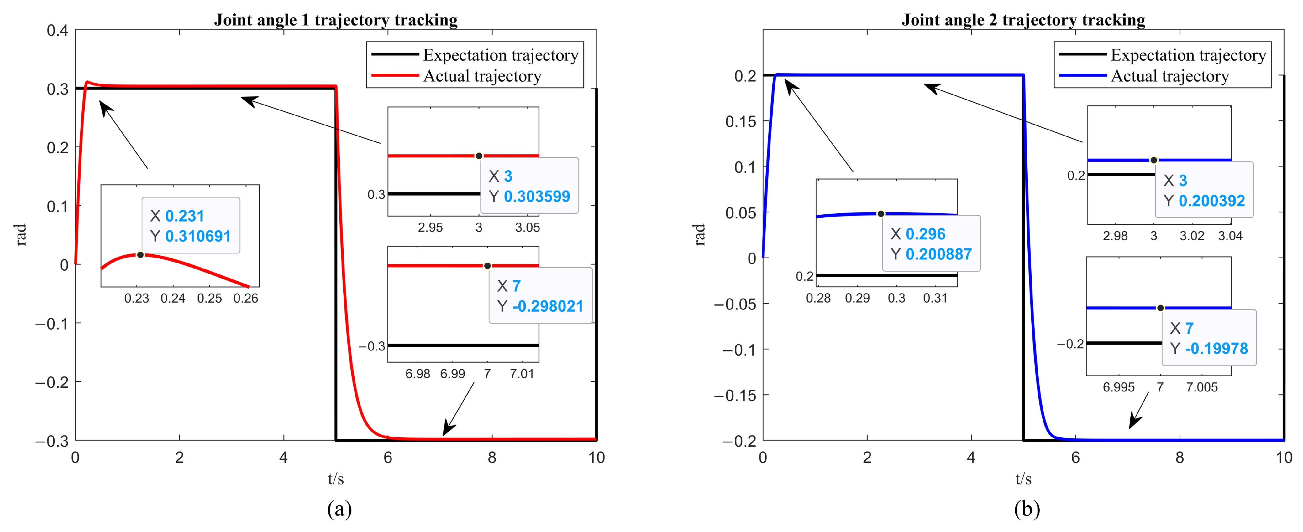
From Figure 4a and Figure 5a, it can be observed that the first arm reaches a steady state at 0.231 s when tracking the desired trajectory, with an overshoot of 0.311 rad. The steady state error is $3.59\times {10}^{-3}$ rad for the first 5 s, and $1.97\times {10}^{-3}$ rad for the 5 to 10 s interval. From Figure 4b and Figure 5b, it is noted that the second arm reaches a steady state at 0.296 s when tracking the desired trajectory, with an overshoot of $2.0088\times {10}^{-1}$ rad. The steady state error is $3.92\times {10}^{-4}$ rad for the first 5 s, and $2.2002\times {10}^{-4}$ rad for the 5 to 10 s interval. From Figure 6, it is known that the maximum control torque of the first and second arms does not exceed the input unsaturated signal.

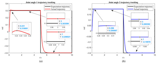
Figure 4. The simulation of the trajectory tracking without the ISSA. (a) The simulation results of the first link. (b) The simulation results of the second link.

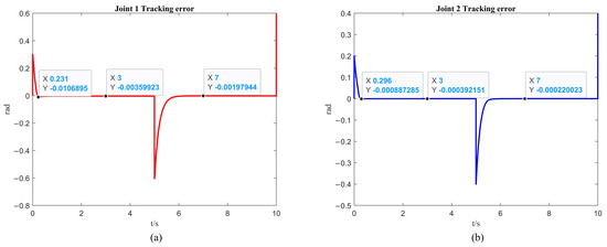
Figure 5. The simulation of the trajectory tracking error without the ISSA. (a) The simulation results of the first link. (b) The simulation results of the second link.

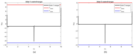
Figure 6. Control torques: (a) the simulation results of the first link; (b) the simulation results of the second link.

A fixed-time improved sparrow search algorithm is employed, with the population size set to 30, and iterated 50 times. For parameters $A_{11}$, $A_{12}$, $A_{21}$, and $A_{22}$, the lower bounds are set to 0.5 times $[0.1,0.01,0.01,0.001]$, and the upper bounds are set to 2 times $[0.1,0.01,0.01,0.001]$. Through multiple iterations and by simulating different controller parameter settings, the corresponding integral of time-weighted absolute error (ITAE) values is calculated. The parameter combination that minimizes the ITAE is selected to achieve the optimization of the overall system.

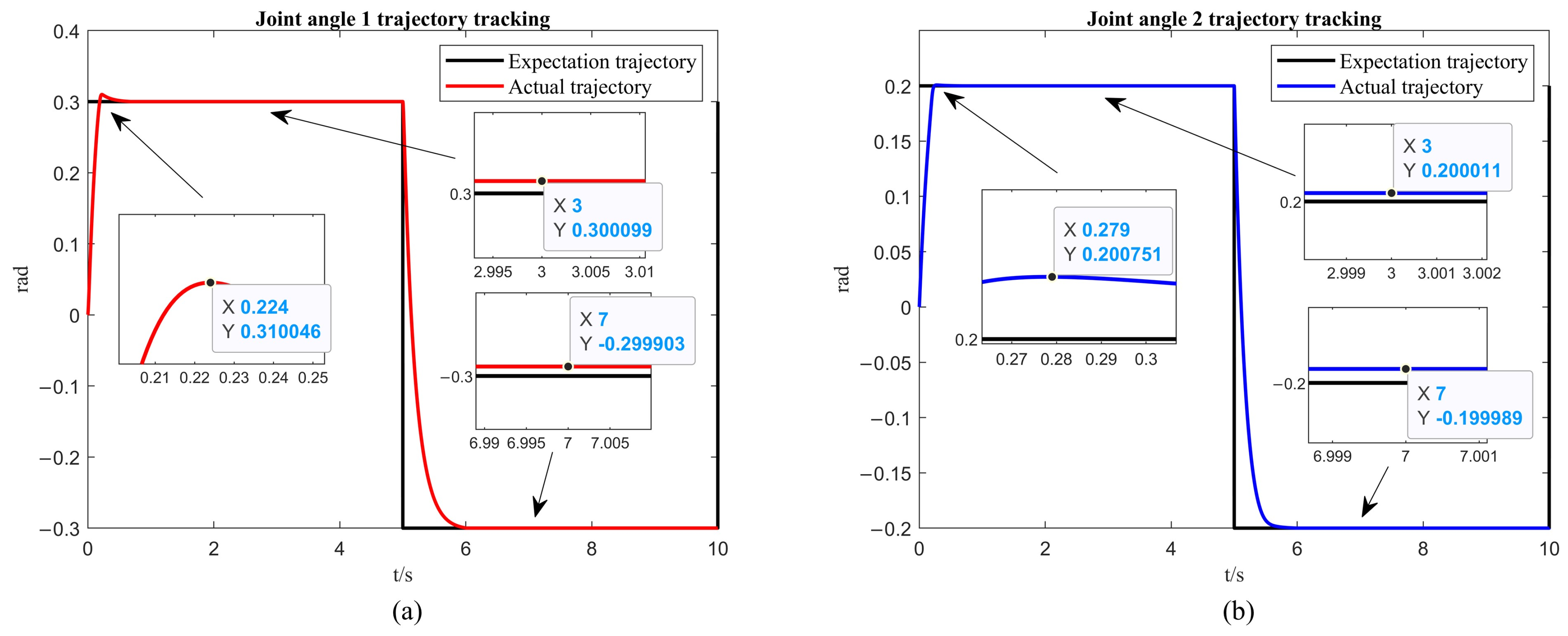
From Figure 7a and Figure 8a, it is observed that the first arm reaches a steady state in 0.224 s while tracking the desired trajectory, with an overshoot of $3.1004\times {10}^{-1}$ rad. The steady state error is $9.86\times {10}^{-5}$ rad for the first 5 s, and $9.68\times {10}^{-5}$ rad for the 5 to 10 s interval. From Figure 7b and Figure 8b, it is noted that the second arm reaches a steady state in 0.279 s while tracking the desired trajectory, with an overshoot of $2.0075\times {10}^{-1}$ rad. The steady state error is $1.075\times {10}^{-5}$ rad for the first 5 s, and $1.076\times {10}^{-5}$ rad for the 5 to 10 s interval.

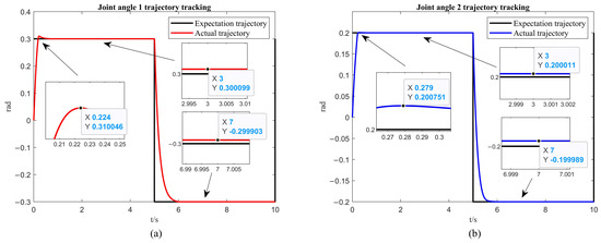
Figure 7. The simulation of trajectory tracking with the ISSA. (a) The simulation results of the first link. (b) The simulation results of the second link.

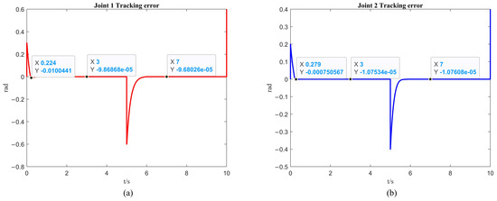
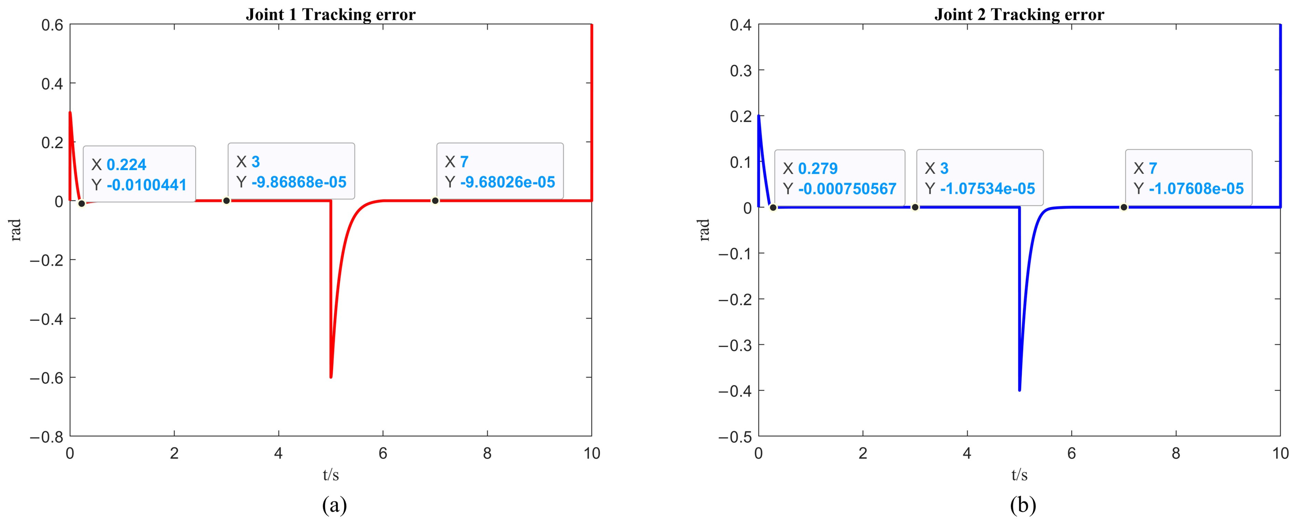
Figure 8. The simulation of trajectory tracking errors with the ISSA. (a) The simulation results of the first link. (b) The simulation results of the second link.

To verify its robustness, we conducted additional comparative simulations using the PD control algorithm alongside the fixed-time control (FTC) algorithm, with the latter optimized by the ISSA (improved sparrow search algorithm). By comparing the tracking error trajectories of both control methods across two joints, we obtained a more comprehensive understanding of the control performance. The PD control is given as follows:

$${\tau }_i=-K_P\left(q_i-q_{id}\right)-K_D{\dot{q}}_i,i=\mathrm{1,2}$$

(59)

where $K_P$ and $K_D$ represent the proportional gain and differential gain, respectively. The control gains are set to $K_P=43$ and $K_D=11.8$. Figure 9 presents the corresponding results of the simulations.

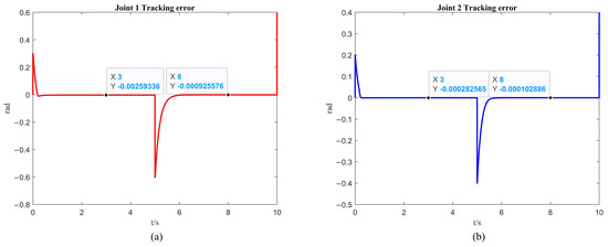
Figure 9. The simulation of PD control: (a) the simulation results of the first link; (b) the simulation results of the second link.

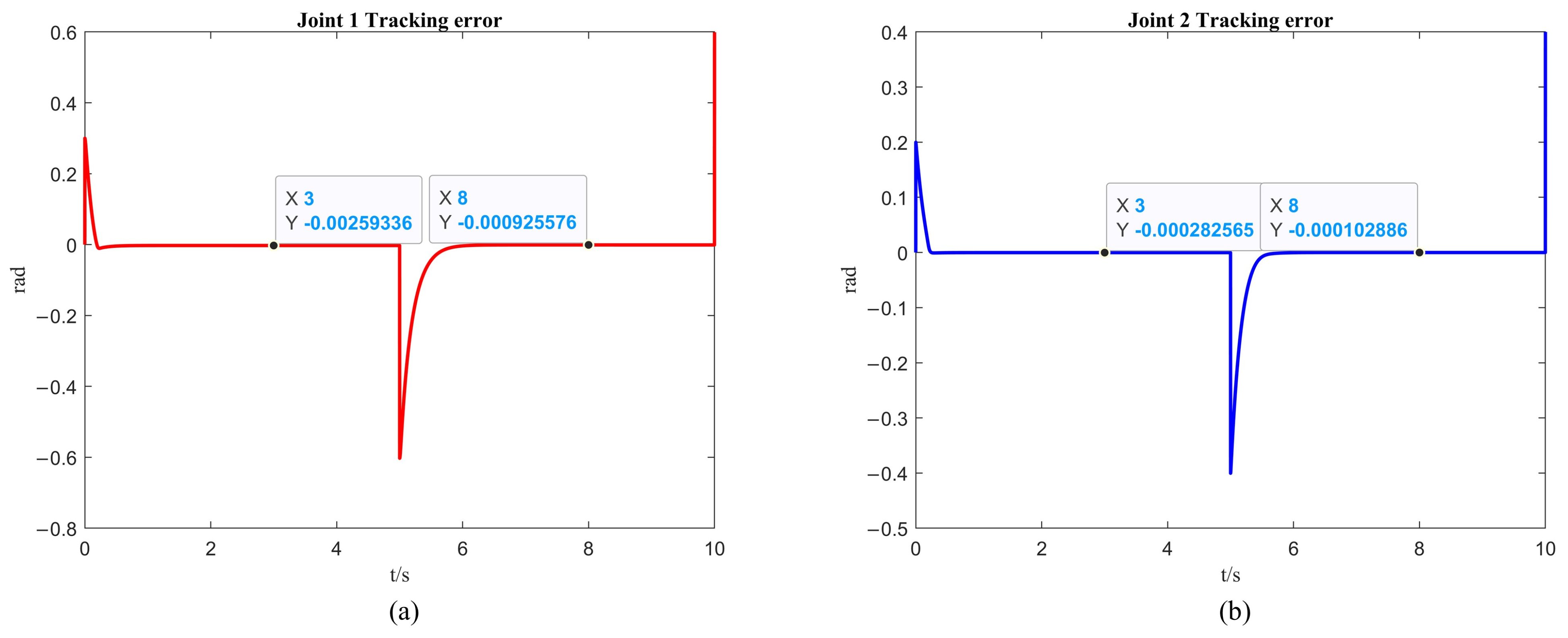
By comparing Figure 9a and Figure 10a, it can be observed that at 3 s, the trajectory errors of the first link of the robotic arm are $-2.59\times {10}^{-3}\mathrm{r}\mathrm{a}\mathrm{d}$ and $-9.87\times {10}^{-5}\mathrm{r}\mathrm{a}\mathrm{d}$, respectively, while at 8 s, the errors are $-9.26\times {10}^{-4}\mathrm{r}\mathrm{a}\mathrm{d}$ and $-9.68\times {10}^{-5}\mathrm{r}\mathrm{a}\mathrm{d}$. Similarly, from the comparison between Figure 9b and Figure 10b, it can be observed that at 3 s, the trajectory errors of the second link of the robotic arm are $-2.83\times {10}^{-4}\mathrm{r}\mathrm{a}\mathrm{d}$ and $-1.08\times {10}^{-5}\mathrm{r}\mathrm{a}\mathrm{d}$, respectively, while at 8 s the errors are $-1.03\times {10}^{-4}\mathrm{r}\mathrm{a}\mathrm{d}$ and $-1.08\times {10}^{-5}\mathrm{r}\mathrm{a}\mathrm{d}$.

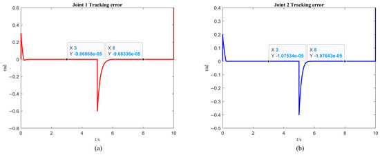
Figure 10. The simulation of fixed-time control with ISSA: (a) the simulation results of the first link; (b) the simulation results of the second link.

It is evident that the steady-state error of the robotic arm under the fixed-time control combined with ISSA is smaller than that under PD control.

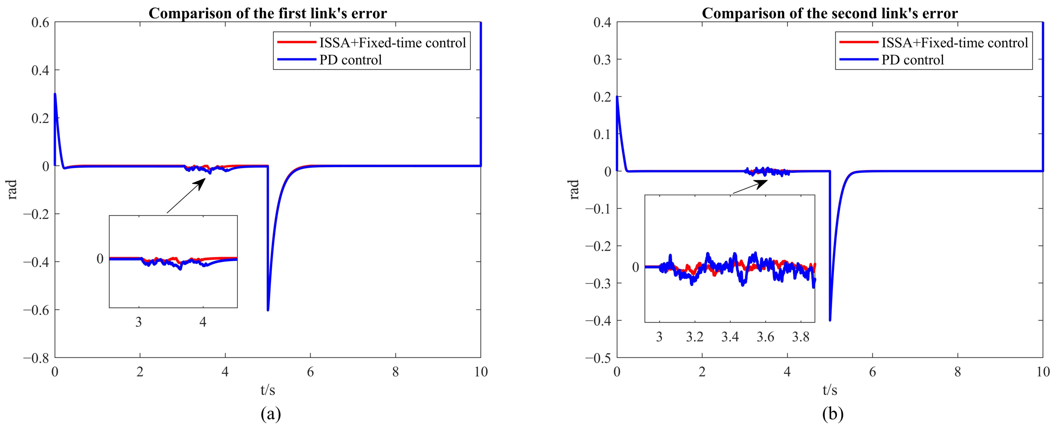
To further demonstrate the robustness of the FTC with ISSA, we introduced external disturbances to the two-DOF robotic arm and compared its performance with that of the PD control. This comparison highlights the superior robustness of the FTC-ISSA method under external interference conditions, as reflected in the error convergence and tracking accuracy metrics.

To simulate potential external disturbances that the system might encounter in real-world operations, a random external disturbance force $F_d$ was applied during the 3 to 4 s interval to evaluate the robustness and stability of the control system. The disturbance force acts on both joints of the robotic arm, with each component affecting one of the two degrees of freedom. The disturbance values are constrained within the range of [−10,10] N, ensuring that the magnitude of the perturbation remains within a physically reasonable range. In certain cases, a hyperbolic tangent (tanh) function was used to smooth the randomly generated disturbance, preventing abrupt changes and simulating more continuous and gradual environmental disturbances. These disturbances are introduced into the system’s dynamic equation, directly influencing the joint acceleration $\ddot{q}$, which in turn alters the overall system trajectory. By introducing such disturbances, the control system’s ability to handle uncertainties and maintain performance under external perturbations is rigorously tested, thus assessing the system’s robustness in unpredictable environments.

As shown in Figure 11a,b, the PD control is subjected to larger disturbances compared to the control method combining ISSA and fixed-time control. The errors induced by the disturbances to both the first and second arms of the robotic system are the largest under PD control. Furthermore, the convergence rate after the disturbance is removed is significantly slower under PD control. This clearly demonstrates the superior robustness of the combined ISSA and fixed-time control in handling uncertainty.

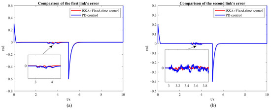
Figure 11. A comparison of errors between ISSA combined with fixed-time control and PD control under external disturbances. (a) The simulation results of the first link. (b) The simulation results of the second link.

4.3. Summary

Compared to two different control methods, it can be concluded that the integration of the ISSA algorithm improves the tracking precision of the first arm by two orders of magnitude, showing a significant enhancement, and also improves the tracking precision of the second arm. Additionally, the response speed is on average 0.007 s faster for the first arm and 0.017 s faster for the second arm compared to the control without ISSA integration. In summary, the figures show that the time-fixed control achieves the goal of rapid convergence, with good control effects and a torque below the input saturation torque. The integration of the ISSA algorithm also achieves the objectives of enhancing control precision and improving response speed. Table 4 and Table 5 summarize the experimental results.

Table 4. Error summary table.

Time (s)	Error of First Link with Fixed-Time Control (rad)	Error of Second Link with Fixed-Time Control (rad)	Error of First Link with Fixed-Time Control + ISSA (rad)	Error of Second Link with Fixed-Time Control + ISSA (rad)
3	$3.59\times {10}^{-3} \mathrm{r}\mathrm{a}\mathrm{d}$	$3.92\times {10}^{-4} \mathrm{r}\mathrm{a}\mathrm{d}$	$9.87\times {10}^{-5} \mathrm{r}\mathrm{a}\mathrm{d}$	$9.68\times {10}^{-5} \mathrm{r}\mathrm{a}\mathrm{d}$
7	$1.97\times {10}^{-3} \mathrm{r}\mathrm{a}\mathrm{d}$	$2.20\times {10}^{-4} \mathrm{r}\mathrm{a}\mathrm{d}$	$9.68\times {10}^{-5} \mathrm{r}\mathrm{a}\mathrm{d}$	$1.08\times {10}^{-5} \mathrm{r}\mathrm{a}\mathrm{d}$

Table 5. Overshoot summary table.

Time (s)	Error of First Link with Fixed-Time Control (rad)	Error of Second Link with Fixed-Time Control (rad)	Error of First Link with Fixed-Time Control + ISSA (rad)	Error of Second Link with Fixed-Time Control + ISSA (rad)
From 0 to 5 s	$1.07\times {10}^{-2} \mathrm{r}\mathrm{a}\mathrm{d}$	$8.87\times {10}^{-4} \mathrm{r}\mathrm{a}\mathrm{d}$	$1.004\times {10}^{-2} \mathrm{r}\mathrm{a}\mathrm{d}$	$7.50\times {10}^{-4} \mathrm{r}\mathrm{a}\mathrm{d}$

I compared an optimized control that combines ISSA and fixed-time control with traditional PD control, and in terms of both trajectory error and robustness, the former proved to be superior.

5. Conclusions

This paper presents a novel approach to the use of the integrated fixed-time control (FTC) algorithm and the improved sparrow search algorithm (ISSA) to minimize the trajectory tracking errors of robotic arms. By integrating the improved ISSA and the FTC, we presented rapid convergence and precise trajectory tracking performance under stringent constraints. The application of barrier Lyapunov functions (BLFs) has proven effective in ensuring the robustness and stability of the control system against disturbances and model uncertainties. While higher DOF systems offer more comprehensive validation, the proposed control algorithms are scalable and adaptable, and we expect similar performances in 3-DOF and 6-DOF systems. Future work will focus on extending this approach to more complex robotic arms in order to further validate its robustness and real-world applicability.

A computer simulation for the two-DOF robotic arm was performed and we confirmed that the proposed hybrid approach significantly reduced tracking errors and improved response speeds compared with the traditional FTC algorithm alone.

According to the chapter on “Simulation on ISSA Performance”, it is evident that ISSA exhibits excellent optimization capabilities and robustness for the system. From the section on “Two-DOF Robotic Arm Simulation”, it is understood that integrating ISSA with fixed-time control yields relatively precise controller parameters, achieving the objectives of reducing errors and enhancing response speed. Compared with traditional PD control methods, its superior robustness has been verified. Our simulation results confirm that there is an enhanced control performance, showcasing significant reductions in tracking errors and faster system responses. This hybrid approach not only leverages the quick convergence properties of fixed-time control but also capitalizes on the global search capabilities of ISSA, finetuning the control actions in order to adapt them dynamically to changing conditions. This study contributes to the field by demonstrating a scalable and reliable control strategy that enhances the operational efficiency of robotic arms in complex environments, paving the way for broader applications in advanced robotic systems.

References

- Li, R.; Qiao, H.; Knoll, A. A Survey of Methods and Strategies for High-Precision Robotic Grasping and Assembly Tasks—Some New Trends. IEEE/ASME Trans. Mechatron. 2019, 24, 2718–2732. [Google Scholar] [CrossRef]
- Hesse, S.; Werner, C.; Pohl, M.; Mehrholz, J.; Puzich, U.; Krebs, H.I. Mechanical Arm Trainer for the Treatment of the Severely Affected Arm After a Stroke. Am. J. Phys. Med. Rehabil. 2008, 87, 779–788. [Google Scholar] [CrossRef] [PubMed]
- Ding, X.L.; Wang, Y.C.; Wang, Y.B.; Xu, K. A review of structures, verification, and calibration technologies of space robotic systems for on-orbit servicing. Sci. China Technol. Sci. 2021, 64, 462–480. [Google Scholar] [CrossRef]
- Hu, J.S.; Chang, N.Y.C.; Yang, J.J.; Wang, J.J.; Lossio, R.G.; Chien, M.C.; Chang, Y.J.; Kai, C.Y.; Su, S.H. FPGA-based embedded visual servoing platform for quick response visual servoing. In Proceedings of the 2011 8th Asian Control Conference (ASCC), Kaohsiung, Taiwan, 15–18 May 2011; pp. 263–268. [Google Scholar]
- Lacquaniti, F.; Licata, F.; Soechting, J.F. The mechanical behavior of the human forearm in response to transient perturbations. Biol. Cybern. 1982, 44, 35–46. [Google Scholar] [CrossRef]
- Zhou, F.; Tian, X.; Tian, L. Reliability Analysis of Quick Coupler Attached to Rescue Manipulator Arm. In Proceedings of the 2019 International Conference on Quality, Reliability, Risk, Maintenance, and Safety Engineering (QR2MSE), Zhangjiajie, China, 6–9 August 2019; pp. 703–708. [Google Scholar]
- Dai, Y.; Li, S.; Chen, X.; Nie, X.; Rui, X.; Zhang, Q. Three-dimensional truss path planning of cellular robots based on improved sparrow algorithm. Robotica 2024, 42, 347–366. [Google Scholar] [CrossRef]
- Tee, K.P.; Ge, S.S.; Tay, E.H. Barrier Lyapunov Functions for the control of output-constrained nonlinear systems. Automatica 2009, 45, 918–927. [Google Scholar] [CrossRef]
- Lin, H.; Zhao, B.; Liu, D.; Alippi, C. Data-based fault tolerant control for affine nonlinear systems through particle swarm optimized neural networks. IEEE/CAA J. Autom. Sin. 2020, 7, 954–964. [Google Scholar] [CrossRef]
- Lee, H.-W. The Study of Mechanical Arm and Intelligent Robot. IEEE Access 2020, 8, 119624–119634. [Google Scholar] [CrossRef]
- Qiu, Z.-C.; Li, C.; Zhang, X.-M. Experimental study on active vibration control for a kind of two-link flexible manipulator. Mech. Syst. Signal Process. 2019, 118, 623–644. [Google Scholar] [CrossRef]
- Sun, C.; Gao, H.; He, W.; Yu, Y. Fuzzy Neural Network Control of a Flexible Robotic Manipulator Using Assumed Mode Method. IEEE Trans. Neural Netw. Learn. Syst. 2018, 29, 5214–5227. [Google Scholar] [CrossRef]
- Jiao, R.; Chou, W.; Ding, R.; Dong, M. Adaptive robust control of quadrotor with a 2-degree-of-freedom robotic arm. Adv. Mech. Eng. 2018, 10, 1687814018778639. [Google Scholar] [CrossRef]
- Zuo, Z.; Tian, B.; Defoort, M.; Ding, Z. Fixed-time consensus tracking for multiagent systems with high-order integrator dynamics. IEEE Trans. Autom. Control 2017, 63, 563–570. [Google Scholar] [CrossRef]
- Song, Y.; Wang, Y.; Krstic, M. Time-varying feedback for stabilization in prescribed finite time. Int. J. Robust Nonlinear Control 2019, 29, 618–633. [Google Scholar] [CrossRef]
- Wang, Y.; Song, Y.; Hill, D.J.; Krstic, M. Prescribed-time consensus and containment control of networked multiagent systems. IEEE Trans. Cybern. 2018, 49, 1138–1147. [Google Scholar] [CrossRef] [PubMed]
- Wang, Y.; Song, Y. Leader-following control of high-order multi-agent systems under directed graphs: Pre-specified finite time approach. Automatica 2018, 87, 113–120. [Google Scholar] [CrossRef]
- Orquera, M.; Campocasso, S.; Millet, D. Topological Optimization of a Mechanical System with Adaptive Convergence Criterion. In Advances on Mechanics, Design Engineering and Manufacturing III, Proceedings of the International Joint Conference on Mechanics, Design Engineering & Advanced Manufacturing, JCM 2020, Aix en Provence, France, 2–4 June 2020; Roucoules, L., Paredes, M., Eynard, B., Morer Camo, P., Rizzi, C., Eds.; Springer: Berlin/Heidelberg, Germany, 2021. [Google Scholar]
- Moubarak, P.; Ben-Tzvi, P. A globally converging algorithm for adaptive manipulation and trajectory following for mobile robots with serial redundant arms. Robotica 2013, 31, 1299–1311. [Google Scholar] [CrossRef]
- Jin, X. Adaptive fixed-time control for mimo nonlinear systems with asymmetric output constraints using universal barrier functions. IEEE Trans. Autom. Control 2018, 64, 3046–3053. [Google Scholar] [CrossRef]
- Li, J.; Yang, Y.; Hua, C.; Guan, X. Fixed-time backstepping control design for high-order strict-feedback non-linear systems via terminal sliding mode. IET Control Theory Appl. 2017, 11, 1184–1193. [Google Scholar] [CrossRef]
- Meng, D.; Zuo, Z. Signed-average consensus for networks of agents: A nonlinear fixed-time convergence protocol. Nonlinear Dyn. 2016, 85, 155–165. [Google Scholar] [CrossRef]
- Zuo, Z. Nonsingular fixed-time consensus tracking for second-order multi-agent networks. Automatica 2015, 54, 305–309. [Google Scholar] [CrossRef]
- Zuo, Z. Non-singular fixed-time terminal sliding mode control of non-linear systems. IET Control Theory Appl. 2015, 9, 545–552. [Google Scholar] [CrossRef]
- Gharehchopogh, F.S.; Namazi, M.; Ebrahimi, L.; Abdollahzadeh, B. Advances in Sparrow Search Algorithm: A Comprehensive Survey. Arch. Comput. Methods Eng. 2023, 30, 427–455. [Google Scholar] [CrossRef] [PubMed]
- Li, Y.; Ni, Z.; Jin, F.; Li, J.; Li, F. Research on clustering method of improved glowworm algorithm based on good-point set. Math. Probl. Eng. 2018, 2018, 1–8. [Google Scholar] [CrossRef]
- Yue, Y.; Cao, L.; Lu, D.; Hu, Z.; Xu, M.; Wang, S.; Li, B.; Ding, H. Review and empirical analysis of sparrow search algorithm. Artif. Intell. Rev. 2023, 56, 10867–10919. [Google Scholar] [CrossRef]
- Xue, J.; Shen, B. A novel swarm intelligence optimization approach: Sparrow search algorithm. Syst. Sci. Control Eng. 2020, 8, 22–34. [Google Scholar] [CrossRef]
- Kadiyala, K.; Murthy, K. Estimation of regression equation with cauchy disturbances. Can. J. Stat. 1977, 5, 111–120. [Google Scholar] [CrossRef]
- Song, W.; Liu, S.; Wang, X.; Wu, W. An improved sparrow search algorithm. In Proceedings of the 2020 IEEE Intl Conf on Parallel & Distributed Processing with Applications, Big Data & Cloud Computing, Sustainable Computing & Communications, Social Computing & Networking (ISPA/BDCloud/SocialCom/SustainCom), Exeter, UK, 7–19 December 2020. [Google Scholar]
- Chen, X.; Huang, X.; Zhu, D.; Qiu, Y. Research on chaotic flying sparrow search algorithm. J. Phys. Conf. Ser. 2021, 1848, 012044. [Google Scholar] [CrossRef]
- Huang, G.-B.; Siew, C.-K. Extreme learning machine: RBF network case. In Proceedings of the ICARCV 2004 8th Control, Automation, Robotics and Vision Conference, Kunming, China, 6–9 December 2004; Volume 2. [Google Scholar]
- Khalfallah, S.; Ghenaiet, A. Radial basis function-based shape optimization of centrifugal impeller using sequential sampling. Proc. Inst. Mech. Eng. Part G J. Aerosp. Eng. 2015, 229, 648–665. [Google Scholar] [CrossRef]
- Chen, Z.; Huang, F.; Sun, W.; Gu, J.; Yao, B. RBF-Neural-Network-based adaptive robust control for nonlinear bilateral teleoperation manipulators with uncertainty and time delay. IEEE/ASME Trans. Mechatron. 2019, 25, 906–918. [Google Scholar] [CrossRef]
- Yu, J.; Zhao, L.; Yu, H.; Lin, C.; Dong, W. Fuzzy finite-time command filtered control of nonlinear systems with input saturation. IEEE Trans. Cybern. 2017, 48, 2378–2387. [Google Scholar] [CrossRef]
- Chen, Z.; Li, Z.; Chen, C.L.P. Adaptive neural control of uncertain MIMO nonlinear systems with state and input constraints. IEEE Trans. Neural Netw. Learn. Syst. 2016, 28, 1318–1330. [Google Scholar] [CrossRef] [PubMed]
- Kong, L.; He, W.; Dong, Y.; Cheng, L.; Yang, C.; Li, Z. Asymmetric bounded neural control for an uncertain robot by state feedback and output feedback. IEEE Trans. Syst. Man Cybern. Syst. 2019, 51, 1735–1746. [Google Scholar] [CrossRef]
- Zhu, Z.; Xia, Y.; Fu, M. Attitude stabilization of rigid spacecraft with finite-time convergence. Int. J. Robust Nonlinear Control 2011, 21, 686–702. [Google Scholar] [CrossRef]
- Wang, H.-Q.; Chen, B.; Lin, C. Adaptive neural tracking control for a class of stochastic nonlinear systems. Int. J. Robust Nonlinear Control 2014, 24, 1262–1280. [Google Scholar] [CrossRef]
- Gao, H.; He, W.; Zhou, C.; Sun, C. Neural network control of a two-link flexible robotic manipulator using assumed mode method. IEEE Trans. Ind. Inform. 2018, 15, 755–765. [Google Scholar] [CrossRef]
- Keighobadi, J.; Mehran, H.-P.; Javad, F. Adaptive neural dynamic surface control of mechanical systems using integral terminal sliding mode. Neurocomputing 2020, 379, 141–151. [Google Scholar] [CrossRef]
Disclaimer/Publisher’s Note: The statements, opinions and data contained in all publications are solely those of the individual author(s) and contributor(s) and not of MDPI and/or the editor(s). MDPI and/or the editor(s) disclaim responsibility for any injury to people or property resulting from any ideas, methods, instructions or products referred to in the content. |
© 2024 by the authors. Licensee MDPI, Basel, Switzerland. This article is an open access article distributed under the terms and conditions of the Creative Commons Attribution (CC BY) license (https://creativecommons.org/licenses/by/4.0/).