Trajectory-Tracking Control of Unmanned Vehicles Based on Adaptive Variable Parameter MPC

Abstract

Aiming at the problems of the poor trajectory-tracking performance and low control accuracy of unmanned vehicles under complex working conditions, we first estimate the lateral force of tires using the square root cubature Kalman filter (SRCKF) in order to correct the lateral stiffness of the tires online, which reduces the model bias caused by constant lateral stiffness, and then adopt a Gaussian function-based adaptive time-domain model predictive control method to improve the trajectory-tracking control accuracy of unmanned vehicles under complex working conditions. Finally, the proposed control algorithm is validated via Carsim and MATLAB/Simulink joint simulation. The results show that compared with the classical model predictive control (MPC) algorithm, the proposed control algorithm reduces the average lateral tracking error by 73.07% and the peak beta and the peak yaw rate by 50.89% and 47.51%, respectively, so that the unmanned vehicle is able to maintain good tracking performance and control accuracy.

1. Introduction

The advancement and development of automated driving technology, along with the modernization of economic levels, have led to the development of new automobile technology that is becoming more intelligent and electrified. Additionally, unmanned electric vehicles that can operate in challenging environments are being used extensively. With its fully wire-control integrated chassis and independent-driving and -braking capabilities, the unmanned electric vehicle can significantly increase operational accuracy and efficiency, in addition to taking the place of manual labor in challenging conditions [1]. Thus, the key to the development of China’s modern industry is the research and development of unmanned vehicles with autonomous precision operation functions that are suitable for complex working conditions. Trajectory-tracking control is the foundation that enables unmanned vehicles to realize autonomous, precise operation.

Many academics are currently conducting extensive research on trajectory-tracking control techniques. PID control [2], optimal control [3], sliding mode control [4], fuzzy control [5], and other techniques are frequently utilized in trajectory-tracking control. These methods can reduce computational time and simplify the control model. Because of the nonlinearity of the vehicle system, the weight parameters must be modified to account for the system’s ability to adapt to changing operating conditions. Consequently, there is a great deal of reliance on the weight parameters. The most versatile among them is model predictive control (MPC), which possesses the qualities of a predictive model, rolling optimization, and feedback correction. It can handle multi-objective and multi-variable optimization problems with constraints [6], has drawn the interest of numerous academics, and has the widest range of applications. For instance, Xu [7] created a fuzzy MPC controller that enhanced trajectory-tracking accuracy by adaptively modifying the weight coefficients in response to field roads’ curvature. By introducing a gradient-projection technique, Liu [8] et al. decreased the number of iterative steps in the MPC algorithm and increased the trajectory-tracking controllers’ response time. Yan [9] optimized the controller’s overall efficiency by adaptively adjusting the adaptive MPC controller’s predictive time domain based on the curvature of roadways. Li et al.‘s adjustments to the weight matrix of the goal function in the MPC increase the controller’s accuracy and stability [10,11,12]. For the vehicle lane-changing problem with constraints on multiple state quantities, Ji [13] proposed a multi-constrained model predictive trajectory-tracking control method by creating a reference predetermined trajectory based on the trapezoidal acceleration method. However, on low-adhesion roads, the yaw rate does not accurately reflect the lateral stability of the vehicle.

Despite the trajectory-tracking control problem of unmanned vehicles under changes in the road lateral inclination and the coefficient of road adhesion, the above studies have not considered the influence of such road surface factors on the MPC trajectory-tracking controller, and in this regard, in recent years, variable-parameter MPCs have been developed to improve the model accuracy and adaptability to working conditions. Amir et al. [14] used model switching to meet the computational efficiency requirements under complex working conditions and improve tracking performance under simple working conditions, but their method also faced the problem of a loss of precision and accuracy. Some scholars have improved the adaptivity by changing the time domain [15,16] and sampling frequency [17], but this method causes rough changes in control quantity, and the accuracy and reliability of the control inputs are thus difficult to guarantee. Liu [18] established an intelligent vehicle dynamics model considering the roadway inclination and constrained the safety of the vehicle’s sideways inclination, which can effectively prevent the vehicle from rollover in mountainous environments, but the method did not consider the effect of the nonlinear side bias characteristics of tires on the control accuracy. Cui [19] proposed a path-tracking controller with corner envelope constraints, which had better trajectory-tracking accuracy at different coefficients of road adhesion. However, it only took the lateral displacement as the evaluation index, which was prone to the risk of vehicle instability caused by the lateral stability of the vehicle exceeding the envelope under the premise of setting the relaxation factor to ensure a feasible solution. As the above methods all set the weight of each evaluation index as a fixed value, it became difficult to adaptively adjust the vehicle when the driving conditions changed, and thus it was difficult to ensure that the vehicle had good dynamic control performance [20]. When an unmanned vehicle is traveling in a complex mountain environment, the tire cornering stiffness is very easy to change in accordance with the driving status of the body and the road surface adhesion. Li [21] considered the effect of load transfer on tire cornering stiffness and obtained real-time tire cornering stiffness by fitting recursive least square to the current tire slip angle and load transfer, but the method failed to consider the effect of the coefficient of road adhesion on the tire sidewall bias characteristics.

In view of this, in order to enhance the adaptive ability of unmanned vehicles in trajectory tracking under complex working conditions, such as the uncertainty of the road surface attachment coefficient, the large curvature of the reference path, and sideways road inclinations, it is possible to enhance the accuracy of trajectory tracking while ensuring the driving stability of the vehicle. We first establish a trajectory-tracking model of unmanned vehicles considering road lateral inclination angle in view of the road characteristics of complex working conditions. Secondly, the lateral forces of the front and rear tires are estimated based on the square root cubature Kalman filter (SRCKF), and the tire cornering stiffness is corrected in real time according to the lateral force of the tires so as to improve the adaptive ability of the model under complex working conditions. And an adaptive prediction time-domain method based on the Gaussian function is designed, which can adaptively optimize the size of the predicted time domain according to the road surface adhesion coefficient and path curvature. Finally, the proposed Adaptive Model Predictive Control (AMPC) trajectory-tracking control method is validated by the joint simulation of Carsim and MATLAB/Simulink.

2. Unmanned Vehicle Trajectory-Tracking Model

2.1. Unmanned Vehicle Dynamics Model

The foundation for achieving precise tracking control is building an accurate unmanned vehicle dynamics model, which is established, as seen in Figure 1 and Figure 2, while taking the road lateral inclination angle into consideration [18,19]. For the unmanned vehicle model, the following presumptions are made in order to increase control efficiency and model accuracy: a small angle assumption is made for the front wheel turning angle ${\delta }_f$, i.e., $\cos ({\delta }_f)\approx 1$. Since we focus on the traverse and roll motions of the vehicle, for the pitching motion of the vehicle, the pitch angle is assumed to be $\theta \approx 0$.

The unmanned vehicle dynamics model can be expressed as

$$\left\{\begin{array}{l}m{\dot{v}}_y=-m\dot{\phi }{v}_x+mh\ddot{\varphi }+(F_{yf}+F_{yr})-mg\varphi \hfill \\ I_x\ddot{\varphi }=m{a}_{y}h+mgh\varphi -M_x\hfill \\ I_z\ddot{\phi }=l_f{F}_{yf}-l_r{F}_{yr}\hfill \end{array}\right.$$

(1)

where $h$ is the height at the center of mass of the unmanned vehicle, $\varphi$ and $\dot{\varphi }$ are the lateral inclination angle and the rate of change of the lateral inclination angle of the body of the unmanned vehicle, and the lateral inclination angle of the body of the unmanned vehicle is mainly caused by the deformation of the suspension system. $M_x$ is the lateral inclination resistance moment of the suspension system of the body of the unmanned vehicle, $M_x=K_{\varphi }{\varphi }_r+D_{\varphi }\dot{\varphi }$; ${\varphi }_r$ is the lateral inclination angle of the body of the vehicle, ${\varphi }_t$ is the pavement camber ${\varphi }_r=\varphi -{\varphi }_t$, assuming that ${\dot{\varphi }}_t\approx 0$, of which $K_{\varphi }$ is the coefficient of lateral inclination stiffness of the unmanned vehicle and $D_{\varphi }$ is the coefficient of lateral inclination damping. $l_f,l_r$ is the distance between the center of mass and the front and rear axles, respectively; $\dot{\phi }$ is the yaw rate of the vehicle, $a_y={\dot{v}}_y+\dot{\phi }{v}_x-h\ddot{\varphi }$ is the transverse acceleration of the center of mass of the unmanned vehicle; there are $m{a}_y=F_y\cos \varphi$, $F_y$ for the combined force of the tire force in the Y-axis direction. $m$ is the overall mass of the vehicle, and $I_z,I_x$ are the moments of inertia of the unmanned vehicle around the Z-axis and X-axis. $F_{yf}$ and $F_{yr}$ are the lateral forces on the front and rear wheels, respectively, where the lateral tire forces can be approximated as

$$F_{yf}=C_f{\alpha }_f,F_{yr}=C_r{\alpha }_r$$

(2)

$C_f$, $C_r$ are the front and rear wheel tire cornering stiffnesses, and ${\alpha }_f$, ${\alpha }_r$ are the front and rear wheel lateral deflection angles. Therefore, the unmanned vehicle dynamics model in Equation (1) can be further expressed as

$$\left\{\begin{array}{l}{\dot{v}}_y\approx F_y({\displaystyle \frac{1}{m}}+{\displaystyle \frac{h^2}{I_x}})-v_x\dot{\phi }+\left[{\displaystyle \frac{h}{I_x}}(mgh-K_{\varphi })-g\right]\varphi \hfill \\ -{\displaystyle \frac{h}{I_x}}{D}_{\varphi }\dot{\varphi }+({\displaystyle \frac{mg{h}^2}{I_x}}-g){\varphi }_t\hfill \\ \ddot{\phi }\approx \left[l_f{F}_{yf}-l_r{F}_{yr}\right]/I_z\hfill \\ \ddot{\varphi }\approx \left[F_{y}h+mgh(\varphi +{\varphi }_t)-K_{\varphi }(\varphi -{\varphi }_t)-D_{\varphi }\dot{\varphi }\right]/I_x\hfill \end{array}\right.$$

(3)

2.2. Unmanned Vehicle Trajectory-Tracking Model

To represent the relationship between the unmanned vehicle and the reference trajectory, a trajectory-tracking model was established [20], as shown in Figure 2. In Figure 2: $L$ is the pre-sighting distance, ${\psi }_d$ is the desired heading angle, $e_y$ is the distance between the center of mass point of the vehicle and the pre-sighting point $d_p$ on the reference trajectory, and $e_d$ is the distance between the center of mass of the vehicle and the nearest point $d$ on the reference trajectory.

According to the relative position relationship between the vehicle and the reference trajectory, the trajectory-tracking model based on single-point pre-sighting can be obtained as

$$\left\{\begin{array}{l}{\dot{e}}_y=v_y+v_x{e}_{\phi }+L\dot{\phi }\hfill \\ {\dot{e}}_{\phi }=\dot{\phi }-{\dot{\psi }}_d=\dot{\phi }-{\kappa }_d{v}_x\hfill \end{array}\right.$$

(4)

where $e_y$ is the lateral position error, $e_{\phi }$ is the heading angle error, ${\kappa }_d$ is the road curvature of the reference trajectory, and $v_x$ is the longitudinal vehicle speed. The pre-sight distance $L$ is set to adaptively adjust the distance size with the longitudinal vehicle speed [21], denoted as

$$L=v_x\Delta t,L_{\min }\le L\le L_{\max }$$

(5)

where $\Delta t=N_{p}T$, $N_p$ is the MPC controller prediction time domain, and $T$ is the controller sampling time. Take the state variable as $x={\left[\begin{array}{llllll}{v}_y\hfill & \dot{\phi }\hfill & \dot{\varphi }\hfill & \varphi \hfill & e_y\hfill & e_{\phi }\hfill \end{array}\right]}^T$, so that the control variable u = δ_f, the output variable is $y={\left[\begin{array}{ccc}\dot{\phi }& e_y& e_{\phi }\end{array}\right]}^T$, and $w$ is the disturbance variable. Combining Equations (3) and (4) gives the state equation of the trajectory-tracking model of the unmanned vehicle as

$$\left\{\begin{array}{l}\dot{x}=Ax+Bu+w\hfill \\ y=Cx\hfill \end{array}\right.$$

(6)

where

$$\begin{array}{l}A=\left[\begin{array}{llllll}{\displaystyle \frac{(C_f+C_r)(\frac{1}{m}+\frac{h^2}{I_x})}{v_x}}\hfill & {\displaystyle \frac{(l_f{C}_f-l_r{C}_r)(\frac{1}{m}+\frac{h^2}{I_x})}{v_x}}\hfill & {\displaystyle \frac{-h{D}_{\varphi }}{I_x}}\hfill & {\displaystyle \frac{-K_{\varphi }h}{I_x}}-g\hfill & 0\hfill & 0\hfill \\ {\displaystyle \frac{(l_f{C}_f-l_r{C}_r)}{I_z{v}_x}}\hfill & {\displaystyle \frac{({l_f}^2{C}_f-{l_r}^2{C}_r)}{I_z{v}_x}}\hfill & 0\hfill & 0\hfill & 0\hfill & 0\hfill \\ {\displaystyle \frac{h(C_f+C_r)}{I_x{v}_x}}\hfill & {\displaystyle \frac{h(l_f{C}_f-l_r{C}_r)}{I_x{v}_x}}\hfill & {\displaystyle \frac{-D_{\varphi }}{I_x}}\hfill & {\displaystyle \frac{-K_{\varphi }}{I_x}}\hfill & 0\hfill & 0\hfill \\ 0\hfill & 0\hfill & 1\hfill & 0\hfill & 0\hfill & 0\hfill \\ 1\hfill & 0\hfill & 0\hfill & 0\hfill & 0\hfill & v_x\hfill \\ 0\hfill & 1\hfill & 0\hfill & 0\hfill & 0\hfill & 0\hfill \end{array}\right]\\ B={\left[\begin{array}{lllll}-C_f({\displaystyle \frac{1}{m}}+{\displaystyle \frac{h^2}{I_x}})-{\displaystyle \frac{l_f{C}_f}{I_z}}\hfill & -{\displaystyle \frac{h{C}_f}{I_x}}\hfill & 0\hfill & 0\hfill & 0\hfill \end{array}\right]}^T\\ w={\left[\begin{array}{llllll}{\displaystyle \frac{h{K}_{\varphi }{\varphi }_t}{I_x}}\hfill & 0\hfill & {\displaystyle \frac{K_{\varphi }{\varphi }_t}{I_x}}\hfill & 0\hfill & 0\hfill & -{\kappa }_d{v}_x\hfill \end{array}\right]}^{T}C=\left[\begin{array}{llllll}0\hfill & 1\hfill & 0\hfill & 0\hfill & 0\hfill & 0\hfill \\ 0\hfill & 0\hfill & 0\hfill & 0\hfill & 1\hfill & 0\hfill \\ 0\hfill & 0\hfill & 0\hfill & 0\hfill & 0\hfill & 1\hfill \end{array}\right]\end{array}$$

(7)

3. Estimation of Tire Cornering Stiffness

3.1. Nonlinear Characterization of Tires

The correctness of the expression of the nonlinear properties of the tires has a direct impact on the control accuracy of the vehicle model since the road forces on the autonomous vehicle must be passed through the tires [22,23,24,25]. As a result, we decided to use Professor Pacejka’s magic formula to explain the nonlinear structural characteristics of tires. This is how the magic tire formula gets put into expression:

$$\left\{\begin{array}{l}{y}_t=D_t\sin \left\{C_t\arctan \left[B_t{x}_t-E_t(B_t{x}_t-\arctan B_t{x}_t)\right]\right\}\hfill \\ Y(x_t)=y(x_t)+S_v\hfill \\ x_t=X+S_h\hfill \end{array}\right.$$

(8)

where $X$ is the wheel lateral deflection angle; $Y$ is the wheel lateral force; $B_t,C_t,D_t,E_t$ are the stiffness, shape, peak, and curvature factors, respectively; and $S_v,S_h$ is the drift of the curve in the vertical and horizontal directions, respectively.

The Magic Tire formula is used to describe the relationship between the corresponding tire side deflection angle and lateral force under different working conditions, as shown in Figure 3 and Figure 4 below. In Figure 3, it can be seen that if the vertical load has a fixed value of 5 kN, since the size of the road surface attachment coefficient determines the slip limit of the tire [26], the larger the road surface attachment coefficient, the larger the extreme value of the lateral force. As can be seen in Figure 4, when the road surface attachment coefficient is 0.9, the change of vertical load will affect the size of the tire cornering stiffness, and the vertical load will change with the change of the vehicle driving status and body mass, and at the same time, the tire cornering stiffness also changes. If the constant tire cornering stiffness continues to be used for the calculation of the tire force, a large model error will be generated.

When designing the controller, it is difficult to adapt the tire force calculated using linear stiffness to changes in road adhesion and load transfer. Therefore, it is necessary to adaptively adjust the lateral stiffness of the controller based on the real-time tire lateral force.

3.2. Lateral Force Estimation

In order to obtain real-time front and rear tire lateral forces, we designed a lateral force estimator based on SCKF. SCKF is the square root form of CKF, which can guarantee symmetry and a positive semi-qualitative covariance matrix. Compared with the EKF and UKF algorithms, the SCKF algorithm has higher estimation accuracy and filtering stability.

It is assumed that the variation of lateral forces in each tire during vehicle travel is consistent with a Markov process, and the variation is described using a second-order stochastic wandering model.

$$\left(\begin{array}{c}{\dot{F}}_0\\ {\dot{F}}_1\end{array}\right)=\left(\begin{array}{cc}0& 1\\ 0& 0\end{array}\right)\left(\begin{array}{c}{F}_0\\ F_1\end{array}\right)+w_F$$

(9)

where $F_0$ is the tire force to be estimated; $F_1$ is the first-order derivative of $F_0$; $w_F$ is random noise. If the state variable is defined to be $x={\left[\dot{\phi },F_{yf},{\dot{F}}_{yf},F_{yr},{\dot{F}}_{yr}\right]}^T$ and the measurement variable is defined to be $z={\left[a_y,\dot{\phi }\right]}^T$, combining Equations (1) and (9), the state-space equation in discrete form can be expressed as follows:

$$\left\{\begin{array}{l}{x}_k=f(x_{k-1})+{\omega }_{k-1}\hfill \\ z_k=h(x_k)+v_k\hfill \end{array}\right.$$

(10)

where $f(\cdot )$ is the state transfer equation; $h(\cdot )$ is the measurement equation; ${\omega }_{k-1}$ is the process noise with covariance $Q_{k-1}$; $v_k$ is the measurement noise with covariance $R_k$. Using the first-order Euler equation with a sampling time of $T$ to approximate the discretization of the system, the state transfer equation and the measurement equation can be expressed as, respectively:

$$f(x_{k-1})=\left[\begin{array}{c}{x}_{1,k-1}+{\displaystyle \frac{1}{I_z}}(l_f{x}_{2,k-1}-l_r{x}_{4,k-1})T\\ x_{2,k-1}+x_{3,k-1}T\\ x_{3,k-1}\\ x_{4,k-1}+x_{5,k-1}T\\ x_{5,k-1}\end{array}\right]h(x_k)=\left[\begin{array}{c}{\displaystyle \frac{x_{2,k}+x_{4,k}+h\ddot{\varphi }-g\varphi }{m}}\\ x_{1,k}\end{array}\right]$$

(11)

The lateral force estimation based on the SCKF algorithm is implemented as follows.

Step 1: Set the initial value of the state ${\widehat{x}}_{0/0}$ and its error covariance matrix square root factor $S_{0/0}$.

Step 2: Time update.

Calculate the volume points and transfer them using the state transfer equation.

$$\begin{array}{l}{x^i}_{k-1/k-1}={\widehat{x}}_{k-1/k-1}+S_{k-1/k-1}{\xi }_i i=1,2,\dots ,2n\\ {x^{i\ast }}_{k-1/k-1}=f({x^i}_{k-1/k-1})\end{array}$$

(12)

where ${\xi }_i$ is the column $i$ of the volume point weight matrix $(\sqrt{n}{I}_n,-\sqrt{n}{I}_n)$; $I_n$ is the unit matrix of $n\times n$; $n$ is the dimension of the state variable.

Calculate the predicted value of the state and the square root factor of its error covariance matrix:

$$x_{k/k-1}={\displaystyle \frac{1}{2n}}{\displaystyle \sum _{i=1}^{2n}}{x^{i\ast }}_{k/k-1}$$

(13)

$$S_{k/k-1}=qr({X^{i\ast }}_{k/k-1},\sqrt{Q_{k-1}})$$

(14)

where $qr$ denotes $QR$ the decomposition; the weighted center matrix ${X^{i\ast }}_{k/k-1}$ is

$${X^{i\ast }}_{k/k-1}={\displaystyle \frac{1}{\sqrt{2n}}}({x^{1\ast }}_{k/k-1}-{\widehat{x}}_{k/k-1},{x^{2\ast }}_{k/k-1}-{\widehat{x}}_{k/k-1},\cdots {x^{2n\ast }}_{k/k-1}-{\widehat{x}}_{k/k-1})$$

(15)

Step 3: Measurement update.

Update the volumetric points and transfer them using the measurement equation.

$$\begin{array}{l}{x^i}_{k/k-1}={\widehat{x}}_{k/k-1}+S_{k/k-1}{\xi }_i\\ {z^i}_{k/k-1}=h({x^i}_{k/k-1})\end{array}$$

(16)

Calculate the predicted values of the measured variables and the square root factors of their new interest covariance matrices:

$$\begin{array}{l}{z^i}_{k/k-1}={\displaystyle \frac{1}{2n}}{\displaystyle \sum _{i=1}^{2n}{z^i}_{k/k-1}}\\ {S^{zz}}_{k/k-1}=qr(Z_{k/k-1},\sqrt{R_k})\end{array}$$

(17)

where the weighted center matrix $Z_{k/k-1}$ is

$$Z_{k/k-1}={\displaystyle \frac{1}{\sqrt{2n}}}({z^1}_{k/k-1}-{\widehat{z}}_{k/k-1},{z^2}_{k/k-1}-{\widehat{z}}_{k/k-1},\cdots {z^{2n}}_{k/k-1}-{\widehat{z}}_{k/k-1})$$

(18)

Calculate measurement covariance matrix and mutual covariance matrix:

$$\begin{array}{l}{p^{zz}}_{k/k-1}={S^{zz}}_{k/k-1}{({S^{zz}}_{k/k-1})}^T\\ {p^{xz}}_{k/k-1}=X_{k/k-1}{Z^T}_{k/k-1}\end{array}$$

(19)

where the weighted center matrix $X_{k/k-1}$ is

$$X_{k/k-1}={\displaystyle \frac{1}{\sqrt{2n}}}({x^1}_{k/k-1}-{\widehat{x}}_{k/k-1},{x^2}_{k/k-1}-{\widehat{x}}_{k/k-1},\cdots ,{x^{2n}}_{k/k-1}-{\widehat{x}}_{k/k-1})$$

(20)

Calculate the filter gain matrix:

$$K_k={p^{xz}}_{k/k-1}{({p^{zz}}_{k/k-1})}^{-1}$$

(21)

Update the state variables and the square root factor of the error covariance matrix:

$$\begin{array}{l}{\widehat{x}}_{k/k}={\widehat{x}}_{k/k-1}+K_k(z_k-{\widehat{z}}_{k/k-1})\\ S_{k/k}=qr(x_{k/k-1}-K_k{z}_{k/k-1},K_k\sqrt{R_k})\end{array}$$

(22)

3.3. Simulation Verification of Lateral Force Estimation

The designed SCKF estimator was tested by using Carsim and the Matlab/Simulink joint simulation platform, and the two working conditions of a high-adhesion road surface and low-adhesion road surface were set for validation, respectively, in which the high-adhesion condition was set with a road adhesion coefficient of 0.9 and a vehicle speed of 90 km/h, and the low-adhesion condition was set with a road adhesion coefficient of 0.4 and a vehicle speed of 50 km/h. The initial state ${\widehat{x}}_{0/0}={\left[0,0,0,0,0\right]}^T$, the square root of the error covariance was taken as $S_{0/0}={10}^{-3}diag\left[1,1,1,1,1\right]$, the process noise covariance was taken as $Q_{k-1}=diag\left[{10}^{-6},2800,20,2800,20\right]$, and the measurement noise covariance was taken as $R_k=diag\left[{10}^{-2},30\times {10}^{-6}\right]$.

Under this condition, the measured values after considering the measurement noise were used as the measurement inputs to the estimator, and the estimation results of the front and rear tire forces were obtained, as shown in Figure 5 and Figure 6.

In Figure 5 and Figure 6, the SCKF estimator can obtain the front and rear tire lateral forces of the vehicle in real time, and the estimated values can match well with the real values obtained based on Carsim. Therefore, the designed estimator can be used to identify the trend of the front and rear tire lateral forces and provide effective data support for the design of the controller.

3.4. Tire Cornering Stiffness Correction

Repeat the above steps to obtain the estimated values of tire lateral force ${\widehat{F}}_{yf}$ and ${\widehat{F}}_{yr}$. Due to the influence of estimation residuals, the ratio of tire lateral force and lateral deflection angle is directly used to solve the tire cornering stiffness [27,28,29], which is prone to produce singular values. This study adopts the normalization parameter to correct the tire cornering stiffness.

$${\epsilon }_i={\displaystyle \frac{{\widehat{F}}_{yi}-F_{yi}}{\left|{\widehat{F}}_{yi}\right|}}\hspace{1em}i=f,r$$

(23)

In order to avoid singular values of the correction factor with a denominator of 0 and to prevent the correction factor from varying too much [30], the following constraints are placed on ${\epsilon }_i$:

$$\left\{\begin{array}{l}{\epsilon }_i\in (-1,1)\hfill \\ {\epsilon }_i=0\hspace{1em}\alpha \le {0.1}^{\circ }\hfill \end{array}\right.\hspace{1em}i=f,r$$

(24)

In the formula, when the tire side deflection angle is less than 1°, the correction coefficient is set to 0, and the corrected tire cornering stiffness can be expressed as

$${\widehat{C}}_{ci}=(1+{\epsilon }_i)C_{ci}$$

(25)

Thus the modified system equation of state can be obtained as

$$\left\{\begin{array}{l}\dot{x}=\widehat{A}x+\widehat{B}u+w\hfill \\ y=Cx\hfill \end{array}\right.$$

(26)

where $\widehat{A}$ and $\widehat{B}$ are the corrected system state matrix and system control matrix. So far, the tire stiffness is corrected in real time according to the low-cost sensor information, and the vehicle model based on SRCKF tire cornering stiffness correction is obtained, which can reduce the influence of parameter uncertainty on the system and then be embedded in the MPC to improve the accuracy and stability of trajectory tracking, which is used in this study for the design of the subsequent controller.

4. Adaptive Trajectory-Tracking Controller Design

4.1. Unmanned Vehicle Dynamics Model

In this study, the trajectory-tracking controller is designed based on the MPC algorithm to discretize Equation (26):

Discretization of the trajectory-tracking model:

$$\left\{\begin{array}{l}x(k+1)=A_{d}x(k)+B_{d}u(k)+Tw(k)\hfill \\ y(k)=C_{d}x(k)\hfill \end{array}\right.$$

(27)

$$A_d=I+\widehat{A}T,B_d=\widehat{B}T,C_d=C$$

Combining the discrete state variables $x(k)$ with the control variables $u(k)$ gives the new state vector as

$$\xi (k)=\left[\begin{array}{c}x(k)\\ u(k-1)\end{array}\right]$$

(28)

Combining Equations (27) and (28) yields the new equation of state as

$$\left\{\begin{array}{l}\xi (k+1)={\tilde{A}}_d\xi (k)+{\tilde{B}}_d\Delta u(k)+Tw(k)\hfill \\ y(k)={\tilde{C}}_d\xi (k)\hfill \end{array}\right.$$

(29)

$${\tilde{A}}_d=\left[\begin{array}{cc}{A}_d& B_d\\ 0& I\end{array}\right],{\tilde{B}}_d=\left[\begin{array}{c}{B}_d\\ I\end{array}\right],{\tilde{C}}_d=(C_d,0),w={\left[\begin{array}{llllll}{\displaystyle \frac{h{K}_{\varphi }{\varphi }_t}{I_x}}\hfill & 0\hfill & {\displaystyle \frac{K_{\varphi }{\varphi }_t}{I_x}}\hfill & 0\hfill & 0\hfill & -{\kappa }_d{v}_x\hfill \end{array}\right]}^T$$

Let the prediction time domain be $N_p$ and the control time domain be $N_c$. Iterative calculation of the state quantities in the prediction time domain can be obtained:

$$Y(k)=C_{p}X(k)+D_p\Delta U(k)+E_{p}W(k)$$

(30)

$$\begin{array}{c}Y(k)=\left[\begin{array}{c}y(k+1)\\ ⋮\\ y(k+N_p)\end{array}\right],\Delta U(k)=\left[\begin{array}{c}\Delta u(k)\\ ⋮\\ \Delta u(k+N_c-1)\end{array}\right],X(k)=\left[\begin{array}{c}\xi (k)\\ ⋮\\ \xi (k+N_p-1)\end{array}\right]\\ D_p=\left[\begin{array}{cccc}{\tilde{C}}_d{\tilde{B}}_d& 0& \cdots & 0\\ {\tilde{C}}_d{\tilde{A}}_d{\tilde{B}}_d& {\tilde{C}}_d{\tilde{B}}_d& \cdots & 0\\ ⋮& ⋮& \cdots & 0\\ {\tilde{C}}_d{{\tilde{A}}_d}^{Nc}{\tilde{B}}_d& {\tilde{C}}_d{{\tilde{A}}_d}^{Nc-1}{\tilde{B}}_d& \cdots & {\tilde{C}}_d{\tilde{B}}_d\\ ⋮& ⋮& \ddots & ⋮\\ {\tilde{C}}_d{{\tilde{A}}_d}^{Np}{\tilde{B}}_d& {\tilde{C}}_d{{\tilde{A}}_d}^{Np-1}{\tilde{B}}_d& \cdots & {\tilde{C}}_d{{\tilde{A}}_d}^{Np-Nc}{\tilde{B}}_d\end{array}\right]W(k)=\left[\begin{array}{c}Tw(k)\\ ⋮\\ Tw(k+N_c-1)\end{array}\right]\\ E_p=\left[\begin{array}{llll}{\tilde{C}}_d\hfill & 0\hfill & \cdots \hfill & 0\hfill \\ ⋮\hfill & ⋮\hfill & ⋮\hfill & ⋮\hfill \\ {\tilde{C}}_d{{\tilde{A}}_d}^{Np-1}\hfill & {\tilde{C}}_d{{\tilde{A}}_d}^{Np-2}\hfill & \cdots \hfill & {\tilde{C}}_d\hfill \end{array}\right]\\ C_p={\left[\begin{array}{cccccc}{\tilde{C}}_d{\tilde{A}}_d& {\tilde{C}}_d{{\tilde{A}}_d}^2& \cdots & {\tilde{C}}_d{{\tilde{A}}_d}^{Nc}& \cdots & {\tilde{C}}_d{{\tilde{A}}_d}^{Np}\end{array}\right]}^T\end{array}$$

Define the MPC cost function as

$$J=Y^{T}QY+\Delta U^{T}R\Delta U+\rho {\epsilon }^2$$

(31)

where $Q,R$ is the weight matrix; $\epsilon$ is the relaxation factor; $\rho$ is the weight coefficient of the relaxation factor. In order to ensure the feasibility of the MPC controller, the control quantity and control increment are constrained:

$$\left\{\begin{array}{l}\Delta U_{\min }\le \Delta U(t)\le \Delta U_{\max }\hfill \\ U_{\min }\le U(t)+A\Delta U(t)\le U_{\max }\hfill \end{array}\right.$$

The above Equation (31) is transformed into a quadratic optimization problem, and the optimal control sequence that satisfies the trajectory-tracking accuracy and body stability is derived through real-time solving [31].

$$\begin{array}{l}\min J={\displaystyle \sum _k\left[W_{e_{\phi }}{({e_{\phi }}^{\left(k\right)})}^2+W_{e_y}{({e_y}^{\left(k\right)})}^2\right]}\\ \hspace{1em}\hspace{1em}\hspace{1em}+{\displaystyle \sum _k{W}_{{\delta }_f}}{\left[{{\delta }_f}^{(k)}-{{\delta }_f}^{(k-1)}\right]}^2\\ s.t\hspace{1em}\hspace{1em}\left\{\begin{array}{l}T\Delta {\delta }_{f\min }\le \Delta {\delta }_f\le T\Delta {\delta }_{f\max }\hfill \\ {\delta }_{f\min }\le {\delta }_f\le {\delta }_{f\max }\hfill \\ {\alpha }_{\min }-\epsilon \le \alpha \le {\alpha }_{\max }+\epsilon \hfill \end{array}\right.\end{array}$$

(32)

Equation (32) suppresses the lateral error and heading angle error in the trajectory tracking of the unmanned vehicle to ensure the accuracy of trajectory tracking [27,28], and the optimal control sequence of the front wheel angle can be obtained by solving.

4.2. Time-Domain Adaptive Design

As one of the important parameters in the model predictive control algorithm, the prediction time domain $N_p$ and control time domain $N_c$ play a key role in the control accuracy of the algorithm [32]. Therefore, it is necessary to select the corresponding values of $N_p$ and $N_c$ for different controlled objects and different external environments.

When the unmanned vehicle is traveling on the road under low-adhesion conditions, the body stability of the unmanned vehicle should be considered first, and then a larger value of the prediction time domain $N_p$ should be selected so as to predict the farther body traveling state and road information and make corresponding adjustments in time. On the contrary, when traveling on the road under high-adhesion conditions, a smaller prediction time domain $N_p$ has a better control effect, which can improve the trajectory-tracking accuracy of the unmanned vehicle on the current road. At the same time, the selection of the prediction time domain $N_p$ must also consider the influence of the road curvature, and when the curvature of the path tracked by the front side is high, the length of the prediction time domain should be appropriately reduced to improve the real-time performance of the controller in order to ensure the tracking accuracy. In summary, when the unmanned vehicle is traveling in complex working conditions, the size $N_p$ should be adjusted according to the specific road conditions.

The road curvature formula based on the definition of curvature is (Mean Road Curvature, MRC)

$$MRC={\displaystyle \frac{1}{N_p}}{\displaystyle \sum _{i=1}^{N_p}\frac{\left|Y_{ref}{(X_i)}^{″}\right|}{{(1+Y_{ref}{(X_i)}^{\prime 2})}^{\frac{3}{2}}}}$$

(33)

where $Y_{ref}{(X_i)}^{\prime }$ and $Y_{ref}{(X_i)}^{″}$ are the first-order and second-order derivatives of the pre-sighting point, respectively. In order to ensure the real-time performance of the controller [32], this study is based on the centralized and uniformly varying two-dimensional Gaussian function to design the function of the prediction time domain about the road surface adhesion coefficient and road curvature:

$$N_p=round\left(A\exp \left({\displaystyle \frac{{(\mu -{\mu }_{\max })}^2}{{{\sigma }_1}^2}}+{\displaystyle \frac{MR{C}^2}{{{\sigma }_2}^2}}\right)\right)$$

(34)

where $A$ is the upper limit of the prediction time domain, ${\mu }_{\max }$ is the upper limit of the road surface attachment coefficient, ${\sigma }_1$ is the influence factor of the road surface attachment coefficient, and ${\sigma }_2$ is the influence factor of the road curvature. According to the vehicle characteristics of the calibration parameters, the predicted time domain offline database can be obtained, and its three-dimensional distribution is shown in Figure 7.

As shown in Figure 8, the solid line is the reference path, with the same basic parameters as the controller; the larger the control time domain $N_c$ is, the higher the control accuracy is, but at the same time, too large $N_c$ will increase the computational burden of the controller. On the contrary, if $N_c$ is too small, the controller will minimize the average error in the prediction time domain, which will lead to poor tracking accuracy at the current position of the unmanned vehicle.

Therefore, when the MRC is large, $N_c$ can be appropriately increased to provide more time to adjust the control inputs to accommodate the curved paths and improve the control accuracy and stability. Conversely, it is appropriate to decrease $N_c$, which reduces the control system computation [17]. Combined with $N_p$, the control time domain expression is designed as

$$N_c=round\left(\gamma N_p(1+\xi MRC)\right)$$

(35)

where $\gamma$ is the predicted time domain weight coefficient, $0<\gamma <0.5$, $\xi$ is the road curvature gain coefficient, $1<\xi <10$.

5. Adaptive Trajectory-Tracking Controller Design

In this study, CarSim (2020.0) and MATLAB (2022b)/Simulink co-simulation were used as the system test platform to construct the classical MPC controller (MPC), tire cornering stiffness adaptive MPC controller (KF-MPC), and tire cornering stiffness and time domain adaptive MPC controller (KF-AG-MPC), respectively. The basic parameters of the three controllers are set the same: the prediction time domain $N_p=30$, the control time domain $N_c=20$, the upper limit of the pre-scanning distance $L_{\max }=4.5$ m, the lower limit $L_{\min }=0.5$ m, and the sampling time $T=0.02\mathrm{s}$. In order to verify the adaptability of the trajectory-tracking controller in an all-terrain environment, a double-lane road with a variable lateral inclination angle and variable coefficient of road adhesion was set up to test the controller. The longitudinal speed of the unmanned vehicle was 72 km/h; it is assumed that the road surface attachment coefficient is 0.6 in the 0–70 m interval of the road and 0.4 in the 70–200 m interval. The controller framework diagram is shown in Figure 9 below:

In order to verify the reasonableness of the Simulink model of the unmanned vehicle built in this paper, according to the steering transient response experiment (steering disc angle step input), the response characteristics are compared with those of the Carsim model under the working condition of a 50 km/h steering disc angle step, as shown in Figure 10.

As can be seen in Figure 10, the Simulink model of the unmanned vehicle constructed in this study agrees with the trend of the yaw rate and the Beta output from the Carsim vehicle model, which proves that the present model is reasonable.

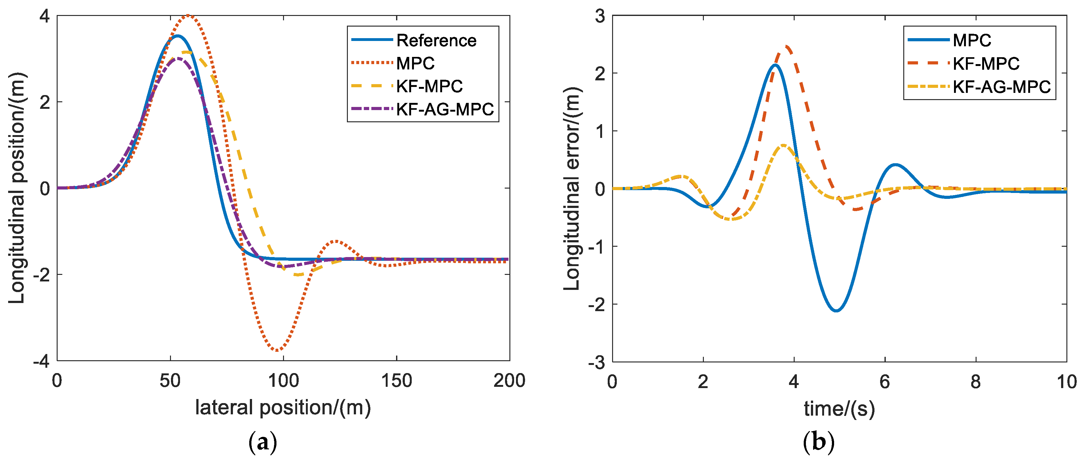
The comparison of the control effects of the three controllers under double-shift conditions is given in Figure 11 and Figure 12 and

Table 1. Control effect comparison.

Evaluation Indicators	MPC	KF-MPC	KF-AG-MPC	Comparison of MPC Optimization Effect
Peak lateral error (m)	−2.11	2.45	0.75	64.46%
Average lateral Error (m)	1.04	0.58	0.28	73.07%
Peak Yaw Rate (deg/s)	−17.41	−14.65	−9.14	47.51%
Peak Beta (deg)	−1.12	0.76	0.55	50.89%

. In Figure 11 and Figure 12, it can be seen that the KF-MPC and KF-AG-MPC have a greater improvement in trajectory-tracking accuracy and vehicle lateral stability compared with the classical MPC controller. This is because the KF-MPC controller can correct tire cornering stiffness in real time according to the driving state of the vehicle, which fully considers the nonlinear characteristics of the tire and greatly reduces the control error caused by the model deviation, while the KF-AG-MPC further improves the trajectory-tracking accuracy and vehicle stability of the vehicle in the curve through the adaptive time domain by taking into consideration the influence of the road surface coefficient of adhesion and the curvature of the road surface on the basis of the KF-MPC. The trajectory-tracking accuracy and vehicle stability are further improved by the adaptive time domain, so that the vehicle is able to improve the tracking accuracy while ensuring the lateral stability of the vehicle under complex working conditions.

The error statistics of the three controllers designed in this study are shown in Table 1, in which the KF-AG-MPC controller has the best control effect. Compared with the classical MPC controller, the peak lateral error is reduced by 64.46%, the average lateral tracking error is reduced by 73.07%, the peak yaw rate is reduced by 47.51%, and the peak Beta is reduced by 50.89%. The control accuracy and stability of the whole vehicle are significantly improved.

Figure 13 and Figure 14 show the adaptive curve of tire cornering stiffness and time domain. In Figure 13, the tire cornering stiffness as a dynamic parameter is corrected in real time along with the driving state of the vehicle, which reflects the time-varying characteristics of the tire cornering stiffness. In Figure 14, the predicted time domain is adaptively adjusted according to the changes in road surface adhesion coefficient and road curvature, which improves the tracking control accuracy.

6. Conclusions

In order to improve the adaptive ability of trajectory-tracking control of unmanned vehicles under complex working conditions, we estimated the tire lateral force online based on the SRCFK algorithm to correct the tire cornering stiffness and realize the real-time correction of the MPC state matrix and the control matrix. The accuracy of the vehicle model in the control algorithm was improved by transforming the complex and unpredictable empirical formula fitting problem into an estimation problem based on the energetic state quantities. The proposed Gaussian-based adaptive time-domain strategy was able to adjust the time-domain size according to the changes in road conditions, which can effectively coordinate the trajectory-tracking accuracy and lateral stability, smoothing the control output and further satisfying the stability requirements of the vehicle.

The simulation experiments of the proposed method were carried out by building a joint simulation model of CarSim and Simulink, and the final experimental results show that, compared with the traditional MPC, the proposed adaptiveness variable-parameter MPC strategy has good adaptive capability and robustness under complex working conditions, and it can greatly improve the tracking accuracy and lateral stability under the double-shifted line condition, which is of great significance for improving the adaptive and robustness of the control system of intelligent automobiles. The proposed adaptive variable-parameter MPC strategy has good adaptive capability and robustness under complex conditions.