(2+1)-Dimensional Fifth-Order KdV Equation and (2+1)-Dimensional Gardner Equation Obtained from Ideal Fluid Model Revisited—Solitary Wave Solutions

Abstract

The (2+1)-dimensional fifth-order KdV equation and (2+1)-dimensional Gardner equation obtained by us using Euler equations for an ideal fluid model in 2023 are revisited. Including additional second-order corrections enabled the derivation of the (2+1)-dimensional fifth-order KdV and Gardner equations without relying on the additional assumptions previously required. The new forms of these equations include an additional non-local term, which allows for the existence of families of solitary wave solutions analogous to solutions to those of the (1+1)-dimensional fifth-order KdV and Gardner equations.

1. Introduction

The physics of non-linear waves is a field of science that has experienced explosive growth during the last half-century. Hundreds of monographs, see, e.g., [1,2,3,4,5,6,7], and many thousands of papers, have been published on the subject. Applications have appeared in many fields, such as hydrodynamics, plasma physics, quantum optics, electric systems, biology, medicine, and neuroscience. Nonlinear wave equations often arise even in first-order approximations of more general fundamental equations that describe a system’s dynamics. The Korteweg–de Vries equation (KdV) [8] is one of the most widely used nonlinear wave equations. It was derived by perturbation theory from a model of an ideal fluid (nonviscous and incompressible) in which the motion is irrotational in the (1+1)-dimension and the bottom of the fluid reservoir is flat. In (2+1)-dimensions, the simplest nonlinear wave equation is the Kadomtsev-Petviashvili equation (KP) [9]. Both the KdV and KP equations are integrable and satisfy many conservation laws. Their analytical solutions are also known.

As nonlinear waves on the surface of seas and oceans are significant in practice, the recent literature contains many papers on (2+1)-dimensional equations. The equations used in these works are often constructed by analogy to the integrable KdV or KP, allowing the authors to construct various types of analytic solutions (solitons, periodic solutions, lumps, and breathers). However, (2+1)-dimensional equations derived from fundamental hydrodynamic equations were not obtained until 2023. In [10], we derived a (2+1)-dimensional extension to the KdV equation for both the flat and uneven bottom. Furthermore, in the case of a flat bottom, we have shown that the KP equation can be obtained from this new (2+1)-dimensional KdV equation through simple differentiation. Therefore, solutions to the (2+1) dimensional KdV equation also satisfy the KP equation. Three families of analytic solutions to this (2+1)-dimensional KdV equation were also found: soliton solutions, periodic cnoidal solutions, and periodic superposition solutions. Additionally, we derived (2+1)-dimensional extensions to the fifth-order KdV equation and the Gardner equation (KdV-mKdV). Next, in [11], we derived the (2+1)-dimensional, extended KdV equation (KdV2) and showed families of soliton, periodic cnoidal, and periodic superposition solutions to this new equation.

In the present paper, we find solitary wave solutions to the fifth-order KdV and Gardner equations. First, in Section 2, we present the full form of the (2+1)-dimensional fifth-order KdV and Gardner equations. Compared with the equations obtained in [10], these contain an additional term, which ensures solutions analogous to the corresponding one-dimensional equations. In Section 3, we derive the solitary wave solutions to the (2+1) dimensional fifth-order KdV equation analogous to the solitary wave solutions to the relevant (1+1) dimensional equation. In Section 4, we do the same for the (2+1)-dimensional Gardner equation. Both Section 3 and Section 4 provide several examples of the solutions found. Section 5 contains the summary and conclusions.

All of the solutions to the (2+1)-dimensional nonlinear wave equations presented in [10,11] and in this paper have the form of traveling waves. Traveling waves in two dimensions have the following general form

$$\eta (x,y,t)=\eta (\pm kx\pm ly\pm \omega t)=\eta (\xi ).$$

(1)

The signs only determine the wave’s propagation direction, leaving its shape and velocity unchanged. Therefore, without loss of generality, we can restrict the consideration to the case $\xi =kx+ly-\omega t$.

2. Full Form of (2+1)-Dimensional Fifth-Order KdV Equation and (2+1)-Dimensional Gardner Equation

Recall the basic set of Euler’s equations for an ideal fluid in the container with a flat, impenetrable bottom [10,11,12]. In dimensional variables, the set of hydrodynamic equations has the following form

$$\hspace{1em}\hspace{1em}\hspace{1em}\hspace{1em}\hspace{1em} {\varphi }_{xx}+{\varphi }_{yy}+{\varphi }_{zz} = 0,\mathrm{in} \mathrm{volume},$$

(2)

$$\hspace{1em}\hspace{1em}\hspace{1em} {\varphi }_z-({\eta }_x{\varphi }_x+{\eta }_y{\varphi }_y+{\eta }_t) = 0,\mathrm{at} \mathrm{the} \mathrm{surface},$$

(3)

$${\varphi }_t+\frac{1}{2}({\varphi }_x^2+{\varphi }_y^2+{\varphi }_z^2)+g\eta +\frac{p_s}{\varrho } = 0,\mathrm{at} \mathrm{the} \mathrm{surface},$$

(4)

$$\hspace{1em}\hspace{1em}\hspace{1em}\hspace{1em}\hspace{1em} {\varphi }_z-h_x{\varphi }_x-h_y{\varphi }_y = 0,\mathrm{at} \mathrm{the} \mathrm{bottom}.$$

(5)

Here, $\varphi (x,y,z,t)$ denotes the velocity potential, $\eta (x,y,t)$ denotes the surface profile function, g is the gravitational acceleration, and $\varrho$ is the density of the fluid. The indexes here and thereafter denote partial derivatives, i.e., ${\varphi }_{xx}\equiv \frac{{\partial }^2\varphi }{\partial x^2}$, ${\eta }_t=\frac{\partial \eta }{\partial t}$, and so on. In (5), $p_s$ is the additional pressure due to the surface tension [13]

$$\begin{array}{cc}\hfill p_s& =-T\nabla ·\left(\frac{\nabla \eta }{{(1+|\nabla \eta |}^2{)}^{1/2}}\right)=T\frac{\left(1+{\eta }_y^2\right){\eta }_{xx}+\left(1+{\eta }_x^2\right){\eta }_{yy}-2{\eta }_x{\eta }_y{\eta }_{xy}}{{\left(1+{\eta }_x^2+{\eta }_y^2\right)}^{3/2}},\hfill \end{array}$$

(6)

where T is the fluid’s surface tension coefficient, and $\nabla =({\partial }_x,{\partial }_y)$ is the two-dimensional gradient.

In the next step, we perform scaling transformation to dimensionless variables

$$\begin{array}{cc}\hfill \tilde{x}=x/L_x,& \tilde{y}=y/L_y,\tilde{z}=z/H,\tilde{t}=t/(L_x/\sqrt{gH}),\hfill \\ \hfill \tilde{\eta }=\eta /A,& \tilde{\varphi }=\varphi /(L_x\frac{A}{H}\sqrt{gH}),\hfill \end{array}$$

(7)

where A is the amplitude of the surface distortions from an equilibrium shape (flat surface), H is the average fluid depth, $L_x$ is the average wavelength (in x-direction), and $L_y$ is a wavelength in the y-direction. In general, $L_y$ should be in the same order as $L_x$, but not necessarily equal. Then, set (2)–(5), in scaled variables, takes the following form (here and thereafter, we omit the tilde signs and work in dimensionless variables) set yields

$$\hspace{1em}\hspace{1em}\hspace{1em}\hspace{1em}\hspace{1em} \beta {\varphi }_{xx}+\gamma {\varphi }_{yy}+{\varphi }_{zz}=0,$$

(8)

$$\hspace{1em}\hspace{1em}\hspace{1em}\hspace{1em}\hspace{1em}\hspace{1em}\hspace{1em}\hspace{1em}{\eta }_t+\alpha ({\eta }_x{\varphi }_x+\frac{\gamma }{\beta }{\eta }_y{\varphi }_y)-\frac{1}{\beta }{\varphi }_z=0,\mathrm{for}z=1+\alpha \eta ,$$

(9)

$${\varphi }_t+\frac{1}{2}\alpha \left({\varphi }_x^2+\frac{\gamma }{\beta }{\varphi }_y^2+\frac{1}{\beta }{\varphi }_z^2\right)+\eta -\tau (\beta {\eta }_{xx}+\gamma {\eta }_{yy})=0,\mathrm{for}z=1+\alpha \eta ,$$

(10)

$$\hspace{1em}\hspace{1em}\hspace{1em}\hspace{1em}\hspace{1em}\hspace{1em}\hspace{1em}\hspace{1em}\hspace{1em}\hspace{1em}\hspace{1em}\hspace{1em}\hspace{1em}\hspace{1em}\hspace{1em}\hspace{1em}{\varphi }_z=0,\mathrm{for}z=0.$$

(11)

Here, $\alpha =\frac{A}{H}$, $\beta ={\left(\frac{H}{L_x}\right)}^2$, and $\gamma ={\left(\frac{H}{L_y}\right)}^2$. Equation (10) contains surface tension effects (see, e.g., [12]), which are important for waves on the surface of thin liquid layers (depths of the order of millimetres). For ordinary shallow water waves (depths of the order of metres, $\tau \in ({10}^{-8}-{10}^{-6})$), surface tension effects can be safely neglected by setting $\tau =0$. Here, $\tau =\frac{T}{\varrho g{H}^2}$ is the Bond number. T is the surface tension coefficient, $\varrho$ is the density of the fluid, g is the gravitational acceleration, and H is the depth of the fluid. In (10), we retained only first- and second-order terms originating from the surface tension, neglecting other terms of the order $O({\beta }^4)$, see the details in Appendix A of [12].

Dimensionless variables allow meaningful approximations to be introduced when solving the complex system of Equations (8)–(11). If we restrict ourselves to the cases where $\alpha ,\beta ,\gamma \ll 1$, it is possible to obtain the corresponding wave equations in any order with respect to these parameters. However, the different ordering of these small parameters leads to different final wave equations, as shown by the authors of [14].

The velocity potential is sought in the form of power series in the vertical coordinate

$$\varphi (x,y,z,t)={\displaystyle \sum _{m=0}^{\infty }}{z}^m{\varphi }^{(m)}(x,y,t),$$

(12)

where ${\varphi }^{(m)}(x,y,t)$ are yet unknown functions. The Laplace Equation (8) and the boundary condition at the bottom (11) determine $\varphi$ in a form that involves only one unknown function, specifically the one with the lowest m-index, $f(x,y,t):={\varphi }^{(0)}(x,y,t)$, along with its space derivatives. Hence,

$$\begin{array}{cc}\hfill \varphi (x,y,z,t)& ={\displaystyle \sum _{m=0}^{\infty }}\frac{{(-1)}^m}{(2m)!}{z}^{2m}{\left(\beta {\partial }_{xx}+\gamma {\partial }_{yy}\right)}^{m}f(x,y,t)\hfill \\ & =f-\frac{1}{2}{z}^2\left(\beta f_{2x}+\gamma f_{2y}\right)+\frac{1}{24}{z}^4\left({\beta }^2{f}_{4x}+2\beta \gamma f_{2x2y}+{\gamma }^2{f}_{4y}\right)\hfill \\ & -\frac{1}{720}{z}^6\left({\beta }^3{f}_{6x}+3{\beta }^2\gamma f_{4x2y}+3\beta {\gamma }^2{f}_{2x4y}+{\gamma }^3{f}_{6y}\right)+\cdots \hfill \end{array}$$

(13)

Next, inserting the velocity potential (13) into (9) and (10), one obtains the set of Boussinesq’s equations whose shape depends on the ordering of small parameters.

2.1. (2+1)-Dimensional Fifth-Order KdV Equation

Assume $\alpha \approx \gamma \approx {\beta }^2$, as in Section 5 of [10]. Then, retaining terms up to the second order in $\beta$, in [10], we obtained the following set of the Boussinesq equations

$$u_t+w_x-\frac{1}{6}\beta w_{3x}+\frac{\gamma }{\beta }\int w_{yy}dx+\alpha {\left(uw\right)}_x+\frac{1}{120}{\beta }^2{w}_{5x}-\frac{1}{3}\gamma w_{x2y}=0,$$

(14)

$$w_t+u_x-\beta \left(\frac{1}{2}{w}_{2xt}+\tau u_{3x}\right)+\alpha w{w}_x+\frac{1}{24}{\beta }^2{w}_{4xt}-\gamma \left(\frac{1}{2}{w}_{2yt}+\tau u_{x2y}\right)=0,$$

(15)

where $w(x,y,t)={\varphi }_x^{(0)}(x,y,t)$.

To obtain a wave equation for $\eta$, one needs to eliminate w from the set of Boussinesq Equations (14) and (15). In other words, find a $w(\eta ,{\eta }_x,{\eta }_y,\dots )$, such that, when inserted into (14) and (15), the two equations become compatible (identical to a certain order of approximation).

We showed in Section 5 of [10] that with

$$\begin{array}{cc}\hfill w=\eta & +\beta \left(\frac{2-3\tau }{6}\right){\eta }_{xx}-\frac{\gamma }{\beta }\frac{1}{2}\int \left(\int {\eta }_{yy}dx\right)dx+\alpha \frac{1}{4}{\eta }^2+{\beta }^2\left(\frac{12-20\tau -15{\tau }^2}{120}\right){\eta }_{4x}\hfill \\ & +\gamma \left(\frac{2-3\tau }{12}\right){\eta }_{yy}+\frac{{\gamma }^2}{{\beta }^2}\frac{3}{8}\int (\int (\int (\int {\eta }_{4y}dx)dx)dx)dx,\hfill \end{array}$$

(16)

Boussinesq Equations (14) and (15) become compatible to the second order in small parameters. Both receive the same form

$$\begin{array}{cc}\hfill {\eta }_t+{\eta }_x& +\beta \left(\frac{1-3\tau }{6}\right){\eta }_{3x}+\frac{\gamma }{2\beta }\int {\eta }_{yy}dx+\frac{3}{2}\alpha \eta {\eta }_x+{\beta }^2\left(\frac{19-30\tau -45{\tau }^2}{360}\right){\eta }_{5x}\hfill \\ & +\gamma \left(\frac{1-3\tau }{4}\right){\eta }_{x2y}-\frac{1}{8}\frac{{\gamma }^2}{{\beta }^2}\int (\int (\int {\eta }_{4y}dx)dx)dx=0.\hfill \end{array}$$

(17)

Strictly speaking, in [10], the last term was missing in w, making the compatibility of Equations (14) and (15) only achievable under the condition ${\eta }_{4y}=0$. The inclusion of a correction term of the order of ${\gamma }^2/{\beta }^2$ has now made it possible to remove this condition and ti obtain the full Equation (17), which is the (2+1)-dimensional extension of the fifth-order Korteweg–de Vries equation derived from the Euler equations describing the irrotational motion of an ideal fluid. Moreover, the presence of this term in (17) ensures the existence of solitary wave solutions to this (2+1)-dimensional wave equation, as shown in Section 3. Without this term, there is no solitary wave solution for Equation (17) (precisely, the assumption of the existence of a soliton solution in the form (23) leads to a contradiction).

2.2. (2+1)-Dimensional Gardner Equation (KdV-mKdV Equation)

Now, assume $\beta \approx \gamma \approx {\alpha }^2$, as in Section 6 of [10]. Then, the Boussinesq equations obtained by retaining terms up to the second order take the following form

$${\eta }_t+w_x+\frac{\gamma }{\beta }\int w_{yy}dx+\alpha {(\eta w)}_x+\frac{\alpha \gamma }{\beta }\left({\eta }_y\int w_{y}dx+\eta \int w_{yy}dx\right)-\frac{1}{6}\beta w_{3x}=0,$$

(18)

$$w_t+{\eta }_x+\alpha w{w}_x+\frac{\alpha \gamma }{\beta }{w}_y\int w_{y}dx-\frac{1}{2}\beta \left(w_{xxt}+2\tau {\eta }_{xxx}\right)=0.$$

(19)

Proceeding as in Section 6 of [10], only supplementing w with a correction term of the order of ${\gamma }^2/{\beta }^2$

$$\begin{array}{cc}\hfill w=u& -\frac{\alpha }{4}{u}^2+\beta \left(\frac{2-3\tau }{6}\right)u_{xx}-\frac{1}{2}\frac{\gamma }{\beta }\int \left(\int u_{yy}dx\right)dx+\frac{{\alpha }^2}{8}{u}^3\hfill \\ & +\frac{\alpha \gamma }{\beta }\left(\frac{5}{8}\int (\int (u_y^2+u{u}_{yy})dx)dx-\frac{3}{8}\int (u\int u_{yy}dx)dx\right)\hfill \\ & +\frac{{\gamma }^2}{{\beta }^2}\frac{3}{8}\int (\int (\int (\int u_{4y}dx)dx)dx)dx\hfill \end{array}$$

(20)

we obtain from Boussinesq’s Equations (18) and (19) the same nonlinear wave equation

$$\begin{array}{cc}\hfill {\eta }_t+{\eta }_x& +\frac{3}{2}\alpha \eta {\eta }_x+\frac{\gamma }{2\beta }\int {\eta }_{yy}dx-\frac{3}{8}{\alpha }^2{\eta }^2{\eta }_x+\frac{1}{6}\beta (1-3\tau ){\eta }_{3x}\hfill \\ & +\frac{\alpha \gamma }{\beta }\left(\frac{1}{8}\int ({\eta }_y^2+\eta {\eta }_{yy})dx+\frac{1}{8}\eta \int {\eta }_{yy}dx+{\eta }_y\int {\eta }_{y}dx-\frac{1}{2}{\eta }_x\int (\int {\eta }_{yy}dx)dx\right)\hfill \\ & -\frac{1}{8}\frac{{\gamma }^2}{{\beta }^2}\int (\int (\int {\eta }_{4y}dx)dx)dx=0.\hfill \end{array}$$

(21)

Equation (21), containing the new (last) term, constitutes the full (2+1)-dimensional Gardner equation, (sometimes referred to as the KdV-mKdV equation). The form published in [10], without this term, was obtained under the condition ${\eta }_{4y}=0$. As in the case of the (2+1)-dimensional fifth-order KdV equation, the presence of a new term ensures the existence of solitary wave solutions to th (2+1) dimensional Gardner Equation (21), as shown in Section 4.

3. Soliton Solutions to (2+1)-Dimensional Fifth-Order KdV Equation

In [11], we found that the form of soliton and periodic solutions to the (2+1)-dimensional KdV and extended KdV equations remain the same as those of (1+1)-dimensional equations. This inspired us to search for solutions to the (2+1)-dimensional fifth-order KdV equation in the same form as solutions for the (1+1)-dimensional fifth-order KdV equation.

Assuming travelling wave solutions in the form (1), that is, $\eta (kx+ly-\omega t)=\eta (x^{\prime }-\omega t)$, one can write Equation (17) as

$$\begin{array}{cc}\hfill {\eta }_t& +\left(k+\frac{\gamma }{2\beta }\frac{l^2}{k}-\frac{{\gamma }^2{l}^4}{8{\beta }^2{k}^3}\right){\eta }_{x^{\prime }}+\frac{3\alpha }{2}k\eta {\eta }_{x^{\prime }}+\left(\frac{\beta }{6}{k}^3+\frac{\gamma }{4}k{l}^2\right)(1-3\tau ){\eta }_{3x^{\prime }}\hfill \\ & +{\beta }^2\left(\frac{19-30\tau -45{\tau }^2}{360}\right)k^5{\eta }_{5x^{\prime }}=0.\hfill \end{array}$$

(22)

Equation (22) is in the form of a one-dimensional fifth-order KdV equation in a fixed reference frame, see Equation (31) of [14]. Therefore, we will look for solutions to Equation (17) in the form analogous to solutions of the one-dimensional fifth-order KdV equation.

So, we postulate travelling wave solutions to (17) as

$$\eta (x,y,t)=A_0+A_4\mathrm{sech}{(kx+ly-\omega t)}^4=A_0+A_4\mathrm{sech}{(\xi )}^4,$$

(23)

where $\xi =kx+ly-\omega t$. For $\eta$, in the form (23), Equation (17) becomes

$$\begin{array}{cc}\hfill & \frac{A_4}{90k^3{\beta }^2}[-45\left(4{\beta }^2{k}^4(3\alpha A_0+2)-8{\beta }^2{k}^3\omega +4\beta \gamma k^2{l}^2-{\gamma }^2{l}^4\right)\hfill \\ & -4{\beta }^2{k}^4{\mathrm{sech}}^4(\xi )\left(135\alpha A_2-94{\beta }^2{k}^4\left(45{\tau }^2+30\tau -19\right)\right)\hfill \\ & +256{\beta }^4{k}^8\left(45{\tau }^2+30\tau -19\right){tanh}^4(\xi )+480{\beta }^2{k}^4(3\tau -1){tanh}^2(\xi )\left(2\beta k^2+3\gamma l^2\right)\hfill \\ & -4{\mathrm{sech}}^2(\xi )\left(262{\beta }^4{k}^8(45{\tau }^2+30\tau -19){tanh}^2(\xi )+105{\beta }^2{k}^4(3\tau -1)(2\beta k^2+3\gamma l^2)\right)]=0.\hfill \end{array}$$

(24)

This equation, when reduced to a single elliptic function, becomes

$$\frac{A_4}{90k^3{\beta }^2}\left(C_0+C_2{\mathrm{sech}}^2(\xi )+C_4{\mathrm{sech}}^4(\xi )\right)=0.$$

(25)

By equating $C_i$ to zero, we obtain three equations for the parameters of the solution (23).

$$\begin{array}{cc}\hfill \hspace{1em}\hspace{1em}\hspace{1em}\hspace{1em}{C}_0=& -180{\beta }^2{k}^4\left(3\alpha A_0+8\gamma l^2(1-3\tau )+2\right)+256{\beta }^4{k}^8\left(45{\tau }^2+30\tau -19\right)\hfill \\ & +960{\beta }^3{k}^6\left(3\tau -1\right)+360{\beta }^2{k}^3\omega -180\beta \gamma k^2{l}^2+45{\gamma }^2{l}^4=0,\hfill \end{array}$$

(26)

$$\hspace{1em}\hspace{1em}\hspace{1em}\hspace{1em} C_2=-60{\beta }^2{k}^4\left(26{\beta }^2{k}^4(45{\tau }^2+30\tau -19)+(30\beta k^2+45\gamma l^2)(3\tau -1)\right)=0,$$

(27)

$$C_4=-60{\beta }^2{k}^4\left(9\alpha A_2-28{\beta }^2{k}^4(45{\tau }^2+30\tau -19)\right)=0.$$

(28)

Then, from (28)

$$A_4=\frac{28{\beta }^2{k}^4\left(45{\tau }^2+30\tau -19\right)}{9\alpha }$$

(29)

and from (27)

$$l^2=-\frac{2\beta k^2\left(13\beta k^2(45{\tau }^2+30\tau -19)-15(1-3\tau )\right)}{45(1-3\tau )\gamma }.$$

(30)

Equation (26), with $l^2$ given by (30), provides

$$\begin{array}{cc}\hfill \omega & =k\left(\frac{3\alpha }{2}{A}_0+\frac{11}{18}-\frac{52\beta k^2\left(45{\tau }^2+30\tau -19\right)}{135(3\tau -1)}\right.\hfill \\ & \left.+\frac{{\beta }^2{k}^4\left(2282175{\tau }^4-456300{\tau }^3-1845990{\tau }^2+1125780\tau -184129\right)}{4050{(1-3\tau )}^2}\right).\hfill \end{array}$$

(31)

We see, that the (2+1)-dimensional fifth-order KdV Equation (17) admits the family of soliton solutions in the form (23). From a mathematical point of view, $A_0$ can be arbitrary. The physical soliton solution, however, requires $A_0=0$ for the volume of the liquid to be the same as that of the undisturbed liquid.

Equation (30) restricts the admissible parameters $k,l$ as l must be real. By definition, see [11], $\beta >0,\gamma >0$, and the bond number $\tau \ge 0$. Then, $l^2>0$ requires

$$\frac{1}{3}<\tau <\frac{-5+2\sqrt{30}}{15}\approx 0.396963\mathrm{and}\left|k\right|>\sqrt{\frac{15(1-3\tau )}{13(45{\tau }^2+30\tau -19)\beta }}.$$

(32)

This means that the soliton solution to the (2+1)-dimensional fifth-order KdV Equation (17) is admissible for thin fluid layers, like in the case of (1+1)-dimensional fifth-order KdV equation.

It is worth noting that the (2+1)-dimensional fifth-order KdV Equation (17) has a whole family of physically meaningful solutions for which conditions (32) and $\alpha ,\beta ,\gamma \ll 1$ are simultaneously satisfied.

The specific conditions on $k,l$ depend on the parameters $\alpha ,\beta ,\gamma$ of Equation (17). Consider a realistic example, when $\alpha =0.2$, $\beta =0.16$, $\gamma =0.05$, and $\tau =0.36$. Then, $l^2\approx -1.77778k^2(0.75-3.88375k^2)$. Then, for $l^2>0$, there must be $\left|k\right|>0.67532$. Take admissible $k=0.7$. Then, $l\approx 0.279$, $A_4\approx -0.16632$ and $\omega \approx 0.705$. With these parameters, the soliton solution (23) with $A_0=0$ is

$$\eta (x,y,t)=-0.16632\mathrm{sech}{(0.7x+0.279y-0.704t)}^4.$$

(33)

Three snapshots of wave profiles for the soliton solution (33) are presented in the left part of Figure 1.

Figure 1. Three snapshots of the soliton solution (33) for (2+1)-dimensional fifth-order KdV equation in two dimensions. Left: Profiles at $t=0,3,6$ in $(x,y)$-coordinates. Right: The same wave profiles are presented in rotated coordinates. For the parameters used in this example, see the details in the text.

Similarly, as in the KdV and extended KdV cases [11], we see that the wave propagates in a direction tilted to the x-axis by the angle $\phi =arctan\left(\frac{l}{k}\right)$. This property is easily seen when coordinates $x^{\prime },y^{\prime }$ are introduced and rotated to $x,y$ by the angle $\phi =arctan\left(\frac{l}{k}\right)$. In these rotated coordinates, we have

$$\begin{array}{cc}\hfill \eta (kx+ly-\omega t)& =\eta \left(k(x^{\prime }cos\phi -y^{\prime }sin\phi )+l(x^{\prime }sin\phi +y^{\prime }cos\phi )-\omega t\right)\hfill \\ & =\eta (\sqrt{k^2+l^2}{x}^{\prime }-\omega t).\hfill \end{array}$$

(34)

In rotated coordinates, the motion is one-dimensional. The wave represented by the function (34) propagates in the $x^{\prime }$-direction, maintaining translational symmetry in the perpendicular $y^{\prime }$-direction. In the example presented in Figure 1, we obtain $\varphi \approx 0.379317$, $\sqrt{k^2+l^2}\approx 0.753565$. The three snapshots of the wave profile presented in Figure 1 are shown along the $x^{\prime }$ direction in the right part of Figure 1.

4. Soliton Solutions to (2+1)-Dimensional Gardner Equation

For the case $\beta =O({\alpha }^2)$, $\gamma =O({\alpha }^2)$, retaining all terms up to the second order in small parameters, in [10], we derived the (2+1)-dimensional Gardner equation

$$\begin{array}{cc}\hfill {\eta }_t+{\eta }_x& +\frac{3}{2}\alpha \eta {\eta }_x+\frac{\gamma }{2\beta }\int {\eta }_{yy}dx-\frac{3}{8}{\alpha }^2{\eta }^2{\eta }_x+\frac{1}{6}\beta (1-3\tau ){\eta }_{3x}-\frac{1}{8}\frac{{\gamma }^2}{{\beta }^2}\int (\int (\int {\eta }_{4y}dx)dx)dx\hfill \\ & +\frac{\alpha \gamma }{\beta }\left(\frac{1}{8}\int ({\eta }_y^2+\eta {\eta }_{yy})dx+\frac{1}{8}\eta \int {\eta }_{yy}dx+{\eta }_y\int {\eta }_{y}dx-\frac{1}{2}{\eta }_x\int (\int {\eta }_{yy}dx)dx\right)=0.\hfill \end{array}$$

(35)

For travelling wave solutions (1), Equation (21) can be written as

$$\begin{array}{cc}\hfill {\eta }_t& +\left(k+\frac{\gamma }{2\beta }\frac{l^2}{k}+\frac{\alpha \gamma }{8\beta }\frac{l^2}{k}-\frac{{\gamma }^2{l}^4}{8{\beta }^2{k}^3}\right){\eta }_{\xi }+\left(\frac{3\alpha }{2}k+\frac{5\gamma l^2}{8\beta k}\right)\eta {\eta }_{\xi }\hfill \\ & -\frac{3{\alpha }^{2}k}{8}{\eta }^2{\eta }_{\xi }+\frac{\beta (1-3\tau )}{6}{k}^3{\eta }_{3\xi }=0,\hfill \end{array}$$

(36)

which has the form of a one-dimensional Gardner equation in a fixed reference frame, see Equation (27) of [14]. Therefore, the (2+1)-dimensional Gardner Equation (21) should have a soliton solution analogous to the one-dimensional Gardner equation.

Postulate solution to (21) in the form analogous to the solution of the one-dimensional Gardner equation, i.e.,

$$\eta (x,y,t)=\frac{A_1}{1\pm A_{2}cosh(kx+ly-\omega t)}=\frac{A_1}{1\pm A_{2}cosh(\xi )}.$$

(37)

Inserting form (37) into (21) leads to the following equation

$$\frac{A_1{A}_{2}sinh(\xi )}{24{\beta }^2{k}^3{(A_{2}cosh(\xi )+1)}^4}\left[C_0+C_{1}cosh(\xi )+C_{2}cosh{(\xi )}^2\right]=0,$$

(38)

where, for abbreviation, we denote $(kx+ly-\omega t)=\xi$. Then, (37) fulfils (21) when all $C_i=0,i=0,1,2$, simultaneously.

Precisely

$$\begin{array}{cc}\hfill \hspace{1em}\hspace{1em}\hspace{1em}{C}_0& =3{\beta }^2{k}^4(3{\alpha }^2{A}_1^2-12\alpha A_1-8)-6\beta \gamma k^2{l}^2(3\alpha A_1+2)\hfill \\ & \hfill -4(6A_2^2-1){\beta }^3{k}^6(3\tau -1)+24{\beta }^2{k}^3\omega +3{\gamma }^2{l}^4=0,\end{array}$$

(39)

$$\begin{array}{cc}\hfill C_1& =-2A_2\left(6{\beta }^2{k}^4(3\alpha A_1+4)+3\beta \gamma k^2{l}^2(3\alpha A_1+4)\right.\hfill \\ & \hfill \left.+8{\beta }^3{k}^6(3\tau -1)-24{\beta }^2{k}^3\omega -3{\gamma }^2{l}^4\right)=0,\end{array}$$

(40)

$$\hspace{1em}\hspace{1em}\hspace{1em}\hspace{1em}{C}_2=A_2^2\left(4{\beta }^3{k}^6(3\tau -1)-24{\beta }^2{k}^4+24{\beta }^2{k}^3\omega -12\beta \gamma k^2{l}^2+3{\gamma }^2{l}^4\right)=0.$$

(41)

Solving the set of Equations (39)–(41) yields

$$\omega =k-\frac{1}{6}\beta k^3(3\tau -1)+\frac{\gamma l^2}{2\beta k}-\frac{{\gamma }^2{l}^4}{8{\beta }^2{k}^3},$$

(42)

$$A_1=-\frac{4{\beta }^2{k}^4(3\tau -1)}{3\alpha \left(2\beta k^2+\gamma l^2\right)},A_2^2=\frac{2{\beta }^3{k}^6(3\tau -1)+12{\beta }^2{k}^4+12\beta \gamma k^2{l}^2+3{\gamma }^2{l}^4}{3{\left(2\beta k^2+\gamma l^2\right)}^2}.$$

(43)

The only restriction on admissible parameters of the solution is the condition $A_2^2>0$, as $A_2$ has to be real for solutions that make physical sense. In general, we have four possible cases corresponding to different physical systems. First, consider the case with $\tau =0$, corresponding to a water depth of meters. For $k,l\ge 0$, the condition $A_2^2>0$ holds when

$$\begin{array}{cc}\hfill & 0<k\le \sqrt{\frac{6}{\beta }}\mathrm{and}l>0\mathrm{or}k>\sqrt{\frac{6}{\beta }}\mathrm{and}l>\sqrt{\sqrt{\frac{2{\beta }^3{k}^6}{3{\gamma }^2}}-\frac{2\beta k^2}{\gamma }}.\hfill \end{array}$$

(44)

The second case, when $\tau$ is of the order of 1/3, corresponds to thin fluid layers. When $0<\tau <\frac{1}{3}$, then $A_2^2>0$ holds when

$$0<k\le \sqrt{-\frac{6}{\beta (3\tau -1)}}\mathrm{and}l>0$$

(45)

$$\mathrm{or}k>\sqrt{-\frac{6}{\beta (3\tau -1)}}\mathrm{and}l>\sqrt{\sqrt{-\frac{2{\beta }^3{k}^6(3\tau -1)}{3{\gamma }^2}}-\frac{2\beta k^2}{\gamma }}.$$

(46)

When $\tau \ge \frac{1}{3}$, then $A_2^2>0$ holds for arbitrary $k,l$. Therefore, for an arbitrary value of the Bond number $\tau$, a family of solutions (37) exists, i.e., there always exist some ranges of admissible values of parameters $k,l$ of solution.

It is worth noting that by changing $k\to -k$ and $l\to -l$, one obtains solutions moving in the opposite directions.

To illustrate possible solutions, consider a particular example. Set, as in Section 3, $\alpha =0.2$, $\beta =0.16$, $\gamma =0.05$. First, assume that $\tau =0$. Choose $k=3,l=2$, admissible by (44) the left part. Then, we have: $A_1\approx 4.4883,A_2\approx 0.88891,\omega \approx 3.9211$. For these coefficients the wave is

$$\eta (x,y,t)=\frac{4.4883}{1+0.88891cosh(3x+2y-3.9211t)}.$$

(47)

In the second example with $\tau =0$, we choose $k=7,l=7$, admissible by (44) the right part. Then, we have $A_1\approx 22.6018,A_2\approx 0.150415,\omega \approx 17.155$. For these coefficients, the wave is

$$\eta (x,y,t)=\frac{22.6018}{1+0.150415cosh(7x+7y-17.155t)}.$$

(48)

Does the (2+1)-dimensional Gardner equation in two dimensions (21) admit table-top soliton solutions for shallow water waves? The answer is yes. Remember that these solutions appear when $A_2\to 0$. In the considered example, when $\alpha =0.2$, $\beta =0.16$, $\gamma =0.05$, we can find such $k,l$, which provide small $A_2\to 0$. For instance, with $k=7,l=6.69886$, we have $A_1\approx 22.8619,A_2\approx 0.000608695,\omega \approx 17.0767$. The wave is

$$\eta (x,y,t)=\frac{22.8619}{1+0.000608695cosh(7x+6.69886y-17.0767t)}.$$

(49)

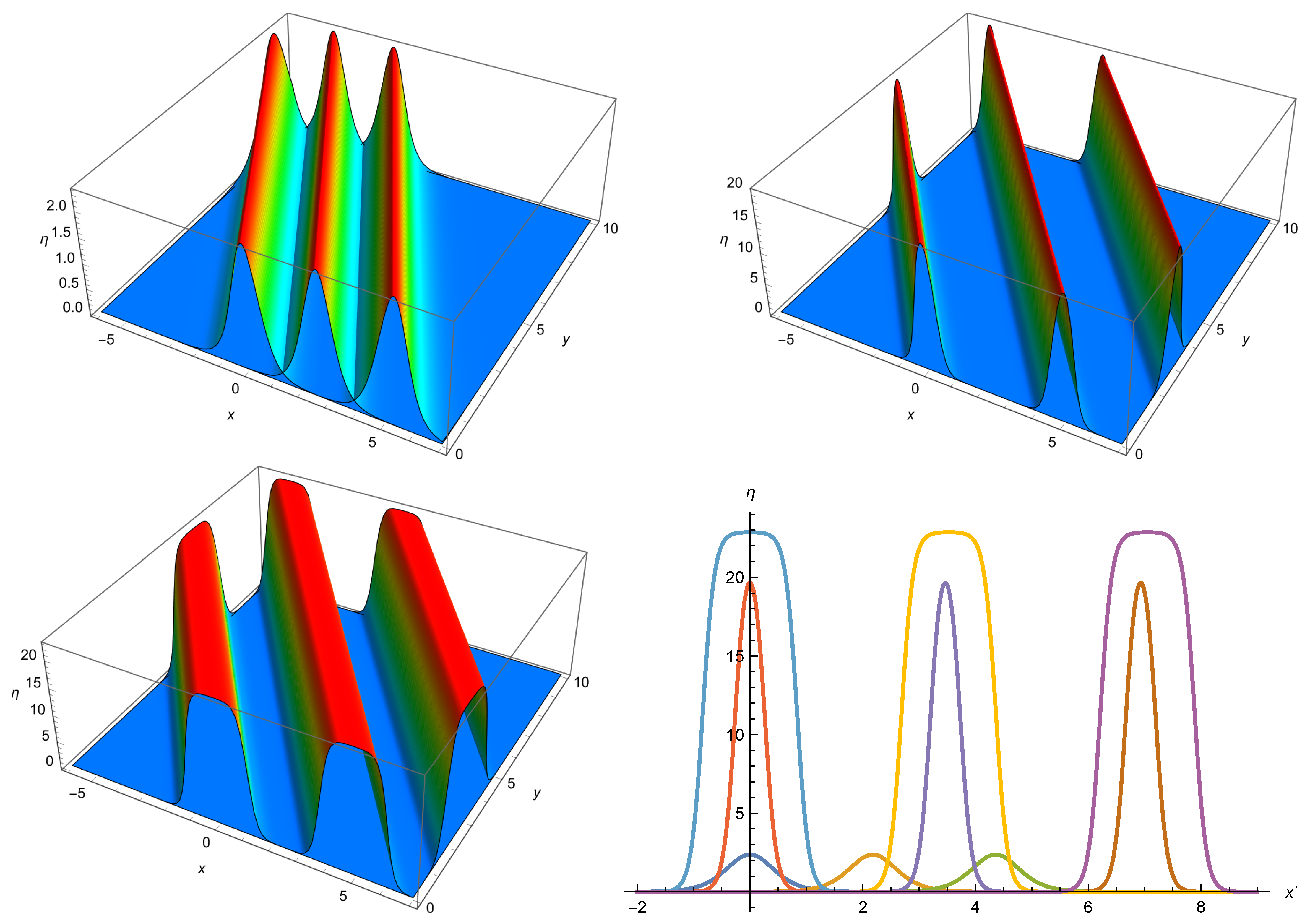
The graphical presentation of these waves is shown in Figure 2. The 3D graphics present three snapshots (overlapped) of the waves’ (47)–(49) profiles. The 2D graphic shows the profiles of these three waves plotted in rotated coordinates. In all three cases, $t=0,2,4$, respectively. The waves exhibit very different amplitudes, widths, and velocities. Therefore, there is a wide family of possible Gardner solitons for the case of shallow water waves, which are related to the case when the surface tension effects can be neglected ($\tau \approx 0$).

Figure 2. Three overlapped snapshots of the solitary wave solutions (37) for (2+1)-dimensional Gardner equation in two dimensions (21). Top left: the wave (47). Top right: the wave (48). Bottom left: the wave (49). Bottom right: Profiles of all three of the considered waves shown in rotated coordinates. All of the wave profiles correspond to time instants $t=0,2,4$.

There are also interesting, physically relevant cases when $\tau$ is close to $\frac{1}{3}$, corresponding to waves on thin fluid layer surfaces. Similar to before, we limited our examples to positive $k,l$. Then, when $\tau <\frac{1}{3}$ the condition $A_2^2>0$ requires

$$k=\sqrt{-\frac{6}{\beta (3\tau -1)}}\mathrm{and}l>0$$

(50)

$$\hspace{1em}\hspace{1em}\hspace{1em}\hspace{1em}\hspace{1em}\hspace{1em}\hspace{1em}\mathrm{or}k>\sqrt{-\frac{6}{\beta (3\tau -1)}}\mathrm{and}l>\sqrt{\sqrt{-\frac{2{\beta }^3{k}^6(3\tau -1)}{3{\gamma }^2}}-\frac{2\beta k^2}{\gamma }}.$$

(51)

Consider a case when $\tau =0.2$ and, as in other examples, $\alpha =0.2,\beta =0.16,\gamma =0.05$. Take $k=10$ and $l=27$, admissible by (51). Then, $A_1=9.97322$, $A_2=0.875716$ and $\omega =25.57$. The solitary wave has the following form

$$\eta (x,y,t)=\frac{9.97322}{1+0.875716cosh(10x+27y-25.57t)}.$$

(52)

When $\tau \ge \frac{1}{3}$, the condition $A_2^2>0$ holds for arbitrary $k,l$. Let us check the solution to the (2+1)-dimensional Gardner equation for $\tau =0.4$ when $k=3$, $l=2$ are the same as in the example of the solution to the (2+1)-dimensional fifth-order KdV equation shown in Figure 1. With these values, (42) and (43) imply $A_1=-0.897662$, $A_2=1.02077$ and $\omega =3.0571$. Then, the solitary wave has the following form

$$\eta (x,y,t)=\frac{-0.897662}{1+1.02077cosh(3x+2y-3.0571t)}.$$

(53)

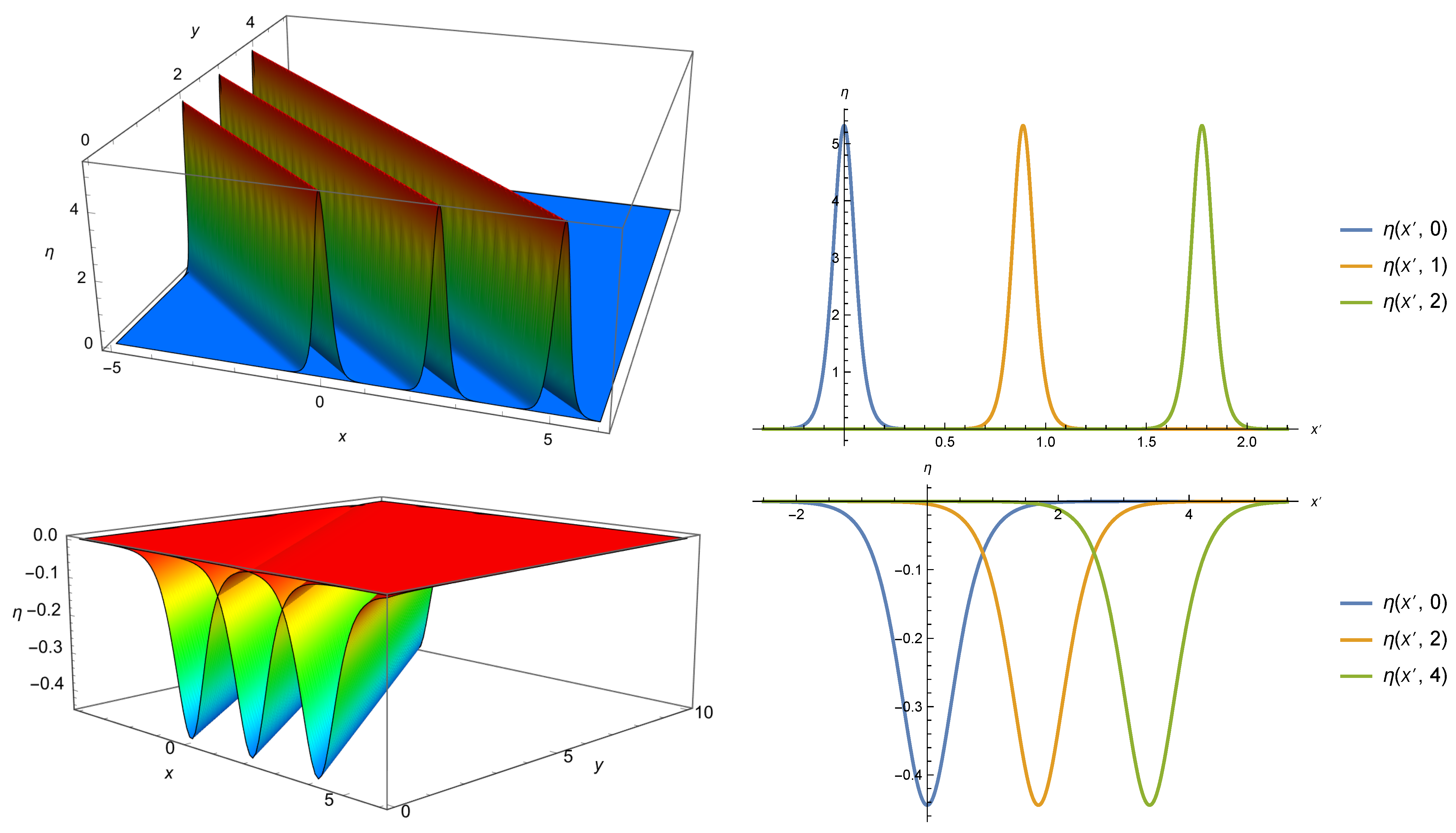
Figure 3 contains a graphical presentation of these solutions. Three snapshots of the wave (52) at $t=0,1,2$ are shown in the top row. Snapshots of the wave (53) at $t=0,2,4$ are shown in the bottom row. The 3D plots are presented in the left column, whereas the one-dimensional motion is shown in rotated coordinates in the right column.

Figure 3. Top row: Three snapshots of the solitary wave solution (52) for the (2+1)-dimensional Gardner equation in two dimensions at $t=0,1,2$. Bottom row: Three snapshots of the solitary wave solution (53) at $t=0,2,4$. Left: 3D plots of $\eta (x,y,t)$. Right: Plots of $\eta (x^{\prime },t)$ in rotated coordinates.

Note that $\tau =\frac{1}{3}$ for water corresponds to $H=H_{\mathrm{crit}}\approx 4.7$ mm. So, according to the (2+1)-dimensional Garnder Equation (21), when $H<H_{\mathrm{crit}}$, the solution has the form of a dark solitary wave, whereas when $H>H_{\mathrm{crit}}$, the solution has the form of a bright solitary wave. The (2+1)-dimensional fifth-order KdV Equation (17) admits only dark solitary wave solutions for $\frac{1}{3}<\tau <\frac{-5+\sqrt{20}}{15}\approx 0.396963$.

5. Summary and Conclusions

The (2+1)-dimensional fifth-order KdV and Gardner equations found in previous work [10] were not complete, i.e., they did not contain all of the possible second-order terms. Equations (17) and (21) in their present form gained soliton solutions analogous to the solutions of the one-dimensional fifth-order KdV and Gardner equations.

It is worth summarizing our results in [10,11] and the current work. We derived (2+1)-dimensional extensions of the famous equations: Korteweg–de Vries Equation (32) of [10], extended KdV Equation (32) of [11], and the full form of 5th-order KdV and Gardner Equations ((17) and (21)). These equations were rigorously derived for the irrotational motion of an ideal fluid. Then, we showed that all the above-mentioned (2+1)-dimensional equations have families of solutions analogous to the corresponding one-dimensional equations. Moreover, though the newly derived equations are explicitly (2+1)-dimensional, the found traveling wave solutions were, in fact, one-dimensional. So, a fundamental question can be posed. Are there other truly two-dimensional solutions to these new equations?

Central to the derivations of these equations is the assumption that the parameter $\gamma ={\left(H/L_y\right)}^2$ is essentially smaller than $\beta ={\left(H/L_x\right)}^2$. In other words, this assumption means that the average wavelength in the y-direction is much larger than that in the x-direction. Only this assumption $\gamma \ll \beta$ allows the system of Boussinesq’s equations to be reduced to a single nonlinear equation for the wave profile. It is possible as y-derivatives do not appear in zeroth order Boussinesq equations.

On the other hand, the assumption $\gamma \ll \beta$ (or $L_y\gg L_x$) is difficult to maintain. It seems that the wave propagation on the water surface should be the same in all directions. However, when $\gamma =\beta$ (or both are of the same order), the Boussinesq equations contain y-derivatives already in the zeroth order [12]. This does not allow us to remove the function $f(x,y,t)$ from the system of Boussinesq equations, which determines the velocity potential, to obtain the wave equation on the surface of the liquid. In principle, approximate solutions $\eta (x,y,t)$ can be obtained indirectly. It is possible to eliminate the surface profile function $\eta (x,y,t)$ from the Boussinesq equations, obtaining the wave equation for the function $f(x,y,t)$. If the solution of this equation was known, then the function $\eta (x,y,t)$ could be obtained from it [12]. However, this problem is much more complicated than those considered so far, and has not yet been solved.