Reinforcement-Learning-Based Trajectory Learning in Frenet Frame for Autonomous Driving

Abstract

Autonomous driving is a complex problem that requires intelligent decision making, and it has recently garnered significant interest due to its potential advantages in convenience and safety. In autonomous driving, conventional path planning to reach a destination is a time-consuming challenge. Therefore, learning-based approaches have been successfully applied to the controller or decision-making aspects of autonomous driving. However, these methods often lack explainability, as passengers cannot discern where the vehicle is headed. Additionally, most experiments primarily focus on highway scenarios, which do not effectively represent road curvature. To address these issues, we propose a reinforcement-learning-based trajectory learning in the Frenet frame (RLTF), which involves learning trajectories in the Frenet frame. Learning trajectories enable the consideration of future states and enhance explainability. We demonstrate that RLTF achieves a 100% success rate in the simulation environment, considering future states on curvy roads with continuous obstacles while overcoming issues associated with the Frenet frame.

1. Introduction

Autonomous driving (AD) is a long-standing challenging problem that requires intelligent decision making to achieve long-term objectives based on the perception of surrounding environments. Recently, AD has received considerable attention, primarily due to its potential advantages in convenience and safety [1,2].

A conventional approach to address AD problems involves the integration of path planning and control. Several methods have proposed a strategy that first plans an optimal path and executes the planned path by using feedback control or model predictive control [3,4,5]. However, those approaches have a drawback in that path planning can be time consuming, particularly for long-horizon plans. In this regard, recently, learning-based approaches have been proposed to train reactive controllers for driving [6,7,8,9]. Hence, once the controller is trained, path planning becomes unnecessary, and autonomous driving can be executed directly using the trained controller.

Learning-based methodologies have successfully trained controllers to perform various autonomous driving tasks, but they still face two primary challenges. Firstly, most of these methods train policies to output abstract low-level commands like steering angles, acceleration/deceleration, or target regions [10,11,12,13]. Consequently, they lack explainability for passengers. For example, in low-level control, the immediate control signals are provided by the policy, making it difficult for passengers to understand where the autonomous vehicle is heading in the future. Similarly, in the case of high-level policies, they express areas like merging zones in merging scenarios or areas to change lanes in lane-changing scenarios, making it equally challenging to convey how the vehicle will maneuver precisely. The second challenge lies in encoding path variations along curves. Most experiments are conducted on highways, where features primarily include surrounding vehicles’ speeds, angles, and accelerations. As a result, these features often fall short in effectively representing the curvature of the road. In environments with pronounced curves, as depicted in Figure 1, the learned policy tends to struggle with generalization.

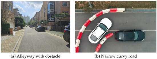
Figure 1. The roads that autonomous driving vehicles might encounter in urban scenarios: (a) a road with continuous obstacles; (b) a narrow, curvy road.

To address explainability and the issues associated with curve-based learning, policies need to model the vehicle’s short-term path. If the policy can provide short-term path predictions, it can offer passengers insights into the future positions of the vehicle, enhancing explainability. Additionally, by verifying whether the policy correctly produces appropriate curves based on curvature, we can assess whether the policy understands curvature correctly. Furthermore, this approach allows for collision checking along the output path in advance, enhancing safety guarantee.

We propose reinforcement-learning-based trajectory learning in the Frenet frame for learning drivable trajectories in complex urban scenarios that require obstacle avoidance on narrow roads with curves, as depicted in Figure 1. To learn trajectories based on curvature, we utilize the Frenet frame. The Frenet frame offers advantages due to its intuitive and convenient nature as it unfolds the coordinate system along a reference line of a road. This allows for the generation of trajectories accommodating various curvatures when a reference line is available. Since the actions of autonomous vehicles must remain consistent within a given state, whether expressed in terms of on-road position or ego-centric coordinates, using the Frenet frame is essential to generate paths compatible with the road [14]. However, it is worth noting that the Frenet frame has some limitations in modeling real-world kinematics and potential distortions in object shapes, making it less suitable for curvy roads [15], which can lead to challenges in obstacle avoidance. We addresses these limitations through reinforcement learning, successfully overcoming them and enabling the effective learning of trajectories for obstacle avoidance.

2. Related Work

Path planning for AD has long been investigated [16]. Path planning is a method used to drive safely from the current state to the goal. To achieve this goal, various path-planning methods have been proposed. The sampling-based approach (e.g., [17,18]) is randomly sampling from the configuration space rather than exploring the entire given environment and then generating the paths based on a given cost function. These methods suffer from generating non-smooth paths and are time-consuming for exploration. Another approach is using polynomials to generate the optimized path (e.g., [19,20]) that considers constraints such as vehicle kinematics. However, this can be computationally expensive. Due to these limitations, various artificial intelligence methods have been recently applied to AVs.

2.1. Supervised Learning for Autonomous Driving

One of the widely applied artificial intelligence methods in AD is learning, including steering angles or trajectories from collected data. For example, Farag et al. [21] learned steering angles using convolution neural networks (CNN) for behavior cloning in the road-following scenarios. Kicki et al. [22] learned executable paths with kinematic constraints to generate paths for a given initial state and desired final state. These methods require pre-collected driving data from expert drivers and cannot outperform the dataset used at the training phase.

2.2. Data-Driven Model Predictive Controller for Autonomous Driving

Data-driven model predictive control (MPC) enhances autonomous driving by using historical data to predict and control vehicle trajectories, eliminating the need for complex modeling. Zhang et al. [23] have proposed the method that uses historical input–output data for efficient trajectory tracking with lower costs compared to traditional methods. Wang et al. [24] developed an algorithm for mixed traffic, which improves traffic flow and fuel efficiency by using driving data without explicit HDV models.

Additional innovations include nonlinear MPC with softened constraints for better stability [25], prediction horizon-varying MPC using proximal policy optimization (PPO) for adaptability [26], and Koopman operator theory to reduce computational burden and enhance accuracy [27]. In particular, Williams et al. [28,29] introduced a model predictive path integral control (MPPI) algorithm for aggressive driving, optimizing nonlinear systems with complex cost criteria. They modeled vehicle dynamics using physics-based analysis and machine learning. This approach fits a Bayesian linear model to historical driving data, capturing key nonlinear behaviors. The MPPI algorithm handles aggressive driving by generating real-time optimal trajectories, validated on a fifth-scale Auto-Rally vehicle Data-driven MPC offers flexibility and robustness, addressing real-world driving complexities more effectively than traditional methods.

2.3. Reinforcement Learning for Autonomous Driving

For this reason, various RL methods are being applied to many tasks in AD [30]. Chen et al. [31] proposed a framework to enable state-of-the-art deep-reinforcement-learning methods (DDQN, TD3, SAC) by encoding the bird-eye-view image into the latent space for driving complex urban scenario. Wang et al. [32] successfully applied DDPG to learn lateral movement in lane-change scenarios, resulting in smooth lane change to the target lane with a 100% success rate in simulations. These methods cannot plan in the long term because the action space consists of control values such as steering angles. Naveed et al. [33] proposed Robust-HRL, which can learn decision making and trajectory for lane-follow/wait and lane-change scenarios. This method does not generate trajectories considering the curvature of the road.

2.4. Frenet Frame for Autonomous Driving

In AD, the Frenet frame, which establishes a coordinate system from a reference line, is widely used for trajectory planning in the road’s curvature [19]. Ye et al. [34] proposed a method for accurately projecting trajectory points onto a reference line in non-differentiable areas with minimal error. Meyer et al. [35] introduced a spatiotemporal GNN model for vehicle-trajectory prediction. Mirchevska et al. [36] learned the parameters of the trajectory planner to generate a trajectory in dynamic highway scenarios with surrounding vehicles having various driver types. Moghadam et al. [37] proposed a method that combines decision-making and motion planning for highway driving in an end-to-end manner in highway scenarios.

In [36,37], parameters were learned using RL for a trajectory planner in the Frenet frame. This is not a trajectory, and requires an additional trajectory planner to generate trajectories. This leads to increased time for trajectory generation. In contrast, our proposed method generates a trajectory as actions, making it more suitable for real time.

3. Backgrounds

3.1. Markov Decision Process

Reinforcement learning can be formulated as a Markov decision process (MDP). An MDP is defined as $⟨\mathcal{S},\mathcal{A},Pr,r⟩$, where $\mathcal{S}$ and $\mathcal{A}$ are set of states and actions, respectively. In our setting, the $Pr:\mathcal{S}\times \mathcal{A}\times \mathcal{S}\mapsto [0,1]$ is a transition probability, and $r:\mathcal{S}\times \mathcal{A}\mapsto \mathbb{R}$ is a reward function.

We will solve the trajectory generation problem in autonomous driving using an MDP. In contrast to the traditional approach where the action is represented as $s\mapsto a$, our proposed method defines $s\mapsto (a_0,a_1,\dots ,a_{K-1})$, where K is the length of the trajectory. The goal of an MDP is to find the optimal policy $\pi$ that maximizes the expected cumulative reward $R(s,\tau )={\mathbb{E}}_{s,a\sim \pi }\left[{\sum }_{t=0}^{T}r(s_t,{\tau }_t)\right]$, where $\tau$ represents the trajectory computed by action.

3.2. Path Generation over Distribution

Since our policy function will be trained to output trajectories, it is essential to model a probability distribution over trajectories. In this regard, Gaussian random paths (GRPs) [38] are mainly utilized to define and sample from the probability distribution at a trajectory level. GRPs utilize Gaussian process regression (GPR) to compute the Gaussian posterior distribution and to model the distribution of paths with a set of M anchoring points $D=(\mathbf{s},\mathbf{x})=\left\{(s_i,x_i)\right|i=1,2,\dots ,M\}$, where $s_i$ and $x_i$ are i-th time index and two-dimensional position, respectively. Given a time T to pass through between the anchoring points, a Gaussian random path $\mathcal{P}$ with a sequence of H test time indices ${\mathbf{t}}_{test}=\{t_i=0,t_1,\cdots ,t_H=T\}$ defines a mean path ${\mu }_{\mathcal{P}}$ and a covariance matrix ${\mathcal{K}}_{\mathcal{P}}$, as follows,

$$\mathcal{P}\sim \mathcal{N}({\mu }_{\mathcal{P}},{\mathcal{K}}_{\mathcal{P}}),$$

(1)

where

$$\begin{array}{cc}\hfill {\mu }_{\mathcal{P}}& =\mathbf{k}{({\mathbf{t}}_{test},\mathbf{s})}^T{({\mathbf{K}}_{\mathbf{s}}+{\sigma }_w^{2}I)}^{-1}\mathbf{x},\hfill \end{array}$$

(2)

$$\begin{array}{cc}\hfill {\mathcal{K}}_{\mathcal{P}}& ={\mathbf{K}}_{test}-\mathbf{k}{({\mathbf{t}}_{test},\mathbf{s})}^T{({\mathbf{K}}_{\mathbf{s}}+{\sigma }_w^{2}I)}^{-1}\mathbf{k}({\mathbf{t}}_{test},\mathbf{s}),\hfill \end{array}$$

(3)

$\mathbf{k}({\mathbf{t}}_{test},\mathbf{s})\in {\mathbb{R}}^{H\times M}$ is a kernel matrix of time indices, where the element is ${\left[\mathbf{k}({\mathbf{t}}_{test},\mathbf{s})\right]}_{(i,j)}=k(t_i,s_j)$, ${\mathbf{K}}_{\mathbf{s}}\in {\mathbb{R}}^{M\times M}$, where the elements are ${\left[{\mathbf{K}}_{\mathbf{s}}\right]}_{(i,j)}=k(s_i,s_j)$ and ${\mathbf{K}}_{test}\in {\mathbb{R}}^{H\times H}$, where the element is ${\left[{\mathbf{K}}_{test}\right]}_{(i,j)}=k(t_i,t_j)$, which is the kernel matrix of anchoring time indices and test time indices, respectively. The trajectory ${\tau }_{grp}$ is generated by sampling from GRPs.

3.3. Frenet Frame

A Frenet frame is a method of constructing a coordinate system along a reference line, which is the center line of a road. Representing a position in the Frenet frame is more intuitive than using a Cartesian frame in autonomous driving. In the Frenet frame, vehicle pose can be expressed as $[b,d,\psi ]$, where b is a longitudinal position from the start of the reference line, d is a lateral position from the reference line, and $\psi$ is an angle between a heading of a car and the reference line, respectively. The comparison between the Cartesian frame and the Frenet frame is shown in Figure 2.

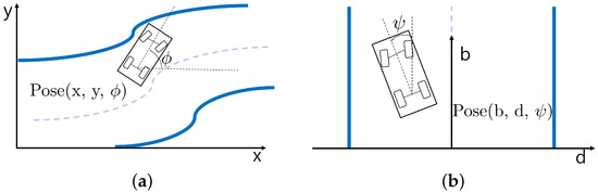
Figure 2. Comparison of Cartesian frame and Frenet frame coordinate representations. The blue line represents the road sideline, and the blue dotted line represents the center of the road. (a) Cartesian frame, (b) Frenet frame.

4. Methods

In this section, we present the reinforcement-learning-based trajectory learning in the Frenet frame (RLTF). In contrast with other methods, the actions of which are parameters of the trajectory planner, the action of RLTF is the trajectory. Furthermore, due to the trajectory generated in the Frenet Frame, RLTF is capable of generating the trajectory in unseen roads in the training phase. Our proposed algorithm overview can be shown in Figure 3.

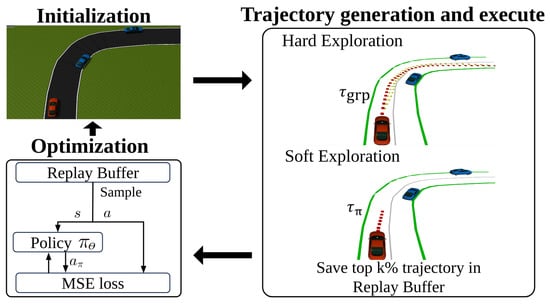
Figure 3. The illustration of the proposed reinforcement-learning-based trajectory learning in the Frenet frame, where ${\tau }_{grp}$ is the trajectory generated by GRPs and ${\tau }_{\pi }$ is the trajectory generated from the policy $\pi$. The action of the policy is optimized to minimize the error with the trajectory in the replay buffer.

4.1. Trajectory Learning

4.1.1. State Space

The state space s consists of the states of the agent vehicle and obstacle vehicles as well as the curvature of the road at the current location and the curvature of the road 15 m ahead. The default values for each agent and obstacles are indicated in the Table 1. The total state dimension is 21, with the agent’s information represented in 4 dimensions and each obstacle vehicle in 5 dimensions. Considering three neighbor vehicles, the obstacle information totals 15 dimensions $(5\times 3)$. Including the 2 dimensions for curvature, the total state space is thus 21 dimensions.

Table 1. State definition of RLTF.

	State Space		Default	Range
Agent	Heading error [rad]	${\psi }_{agent}$	-	$-\pi /2\sim \pi /2$
	Lateral distance [m]	$d_{agent}$	-	$0\sim \infty$
	Distance with front vehicle [m]	$b_{fv}$	30	$0\sim 30$
	Velocity [km/h]	$v_{agent}$	-	$0\sim \infty$
Obstacle	Heading error [rad]	${\psi }_{obs}$	0	$-\pi /2\sim \pi /2$
	Difference with agent [m]	$\Delta x_{obs}$	5.48, −3.16	$5.48\sim 30$ or $-10\sim -3.16$
		$\Delta y_{obs}$	5.48, −3.16	$5.48\sim 30$ or $-10\sim -3.16$
	Lateral distance [m]	$d_{obs}$	40	$0\sim 40$
	Obstacle length in Frenet frame [m]	$le{n}_{obs}$	0	$0\sim \infty$
Curvature	Curvature at current position	${\kappa }_{\mathrm{current}}$	-	$-\infty \sim \infty$
	Curvature at 15m ahead	${\kappa }_{\mathrm{ahead}}$	-	$-\infty \sim \infty$

The agent state includes a heading error in the Frenet frame ${\psi }_{agent}$, the lateral distance in the Frenet frame $d_{agent}$, the distance with the closest front vehicle $b_{fv}$ in the Frenet frame, and the current velocity $v_{agent}$. The obstacle state includes two vehicles within a 30-m range in front of the agent vehicle and one vehicle within a 10-m range behind the agent vehicle. The state of each obstacle vehicle consists of a heading error in the Frenet frame ${\psi }_{ob{s}_z}$, the differences between the agent vehicle and other vehicles after coordinate transform to the agent vehicle $\Delta x_{ob{s}_z},\Delta y_{ob{s}_z}$, the lateral distance in the Frenet frame $d_{ob{s}_z}$, and the length of obstacle vehicle in the Frenet frame $le{n}_{ob{s}_z}$, where z is the z-th obstacle vehicle.

4.1.2. Action Space

The action space consists of:

$$a=(\Delta b,\Delta d)$$

where $\Delta b$ and $\Delta d$ are differences between the current point and next point in the Frenet frame. In practice, the points are recorded from a Cartesian frame and then transformed into the Frenet frame. This action a represents the changes in lateral and longitudinal positions between consecutive time steps. The trajectory is generated by adding the action to the current position of the agent. We refer to it as ${\tau }_{\pi }$. When designing the policy function, it is structured to output the next K actions. Hence, our policy function outputs a $2K$ dimensional vector $(a_{t+1},\cdots ,a_{t+K})$, where t indicates the current time step.

4.1.3. Reward Function

We have designed the reward function to learn trajectories that avoid obstacles as far as possible while considering the vehicle heading constraints. In the absence of obstacles, the objective is for the agent vehicle to follow the center of the road. The rewards are calculated after following the trajectory entirely. The reward function consists of four components as follows:

$$r=r_{\mathrm{success}}+r_{\mathrm{dev}}+r_{\mathrm{cte}}+r_{\mathrm{avoid}}$$

$r_{\mathrm{success}}$ is a reward that indicates whether the agent vehicle is following a successful trajectory. If the agent successfully follows the trajectory to the end, the $r_{\mathrm{success}}$ is 400; otherwise, it is $-500$. $r_{\mathrm{dev}}=-10\times {\displaystyle \frac{1}{b_{\mathrm{end}}-b_{\mathrm{start}}}}{\sum }_{h=0}^H{d}_h$ is a reward that encourages the agent to stay close to the center of the road when there are no obstacles while avoiding veering off the road, where $b_{end}$ and $b_{start}$ are the longitudinal position of the agent at the end and start of each episode, respectively. $H=\left\{h_i|i=1,2,\dots ,H_{end}\right\}$ is recorded every test time step t of the GRP, where $H_{end}$ is when the executed trajectory ends. $d_h$ is $d_{agent}$ at time h. $r_{\mathrm{cte}}=-10\times \mathbb{E}\left[{\sum }_{h=0}^H{e}_h{({\tau }_{any},p_{agent})}_2\right]$ evaluates whether the trajectory can accommodate the heading constraint of the vehicle, where ${\tau }_{any}$ is any trajectory and $e_h({\tau }_{any},p_{agent})$ is the cross-track error between ${\tau }_{any}$ and agent position $p_{agent}$ at time h. A detailed explanation of cross-track error can be found in [39]. $r_{\mathrm{avoid}}=10\times {\sum }_{z=1}^Z{\parallel p_{ob{s}_z}-p_{agent}\parallel }_2$ is an obstacle avoidance reward, with higher values rewarded for successfully avoiding obstacles at a farther distance when obstacles are present, where Z is the total number of obstacle vehicles, $p_{ob{s}_z}$ is the position of the z-th obstacle, and $p_{agent}$ is the position of the agent. $r_{\mathrm{avoid}}$ is computed when the agent vehicle and the obstacle vehicle are at the same b in Frenet frame. Descriptions and value ranges of each reward term are summarized in the Table 2.

Table 2. Summary of reward valuation.

Reward Term	Description	Value Range
$r_{\mathrm{dev}}$	Keeps agent near road center.	−50 to 0 (approx.)
$r_{\mathrm{cte}}$	Checks alignment with road heading [39].	−100 to 0 (approx.)
$r_{\mathrm{avoid}}$	Measures obstacle avoidance.	0 to 100 (approx.)
$r_{\mathrm{success}}$	Rewards reaching end; penalizes collision/off-road.	400 (success), −500 (failure)
r	Combined score from all terms.	−550 to 500 (approx.)

4.2. Trajectory Frame Transform

We need a transformation method between two frames to convert trajectories from the Cartesian frame to the Frenet frame and vice versa. To compute the coordinate in the Frenet frame, the reference line is needed, and it is represented as a polyline. First, we find the nearest point on the reference line to the current position in the current frame and then perform the coordinate transform. The frame transform steps are as follows:

• Find the closest point $l_{\mathrm{current}}\left(i\right)$ to the $p_{\tau }\left(j\right)$ on the reference line in the current frame, where $l_{\mathrm{current}}\left(i\right)$ is position of the ith point on the reference line in current frame and $p_{\tau }\left(j\right)$ is position of the jth point on the trajectory.
• Calculate the difference between that $p_{\tau }\left(j\right)$ and $l_{\mathrm{current}}\left(i\right)$:

  $$[\Delta x_j,\Delta y_j]=p_{\tau }\left(j\right)-l_{\mathrm{current}}\left(i\right)$$
• Compute the angle ${\varphi }_l$ between the $l_{\mathrm{cartesian}}(i+1)$ and the $l_{\mathrm{cartesian}}\left(i\right)$, then rotate $(\Delta x,\Delta y)$ by ${\varphi }_l$:

  $$\left[\begin{array}{c}\Delta x_j^{\prime }\\ \Delta y_j^{\prime }\end{array}\right]=\left[\begin{array}{cc}cos{\varphi }_l& -sin{\varphi }_l\\ sin{\varphi }_l& cos{\varphi }_l\end{array}\right]\left[\begin{array}{c}\Delta x_j\\ \Delta y_j\end{array}\right],$$

  where $l_{cartesian}$ is the reference line in the Cartesian frame. If transforming trajectory from the Cartesian frame to the Frenet frame, then the sign of ${\varphi }_l$ is negative.
• $p_{\tau }\left(j\right)$ is transformed into the target frame by adding the rotated points $(\Delta x_j^{\prime },\Delta y_j^{\prime })$ to the $l_{\mathrm{target}}\left(i\right)$, where $l_{\mathrm{target}}\left(i\right)$ is position of the i-th point on the reference line in the target frame:

  $$p_{\tau }\left(j\right)=l_{\mathrm{target}}\left(i\right)+(\Delta x_j^{\prime },\Delta y_j^{\prime })$$

Trajectories in the Cartesian frame are transformed into the Frenet frame by repeating these steps iteratively, and vice versa.

4.3. Reinforcement-Learning-Based Trajectory Learning in Frenet Frame

In the training phase, the parameter of policy $\theta$ is trained towards maximizing $R(s,{\tau }_{\pi })$. We first generate the replay buffer for the total number of obstacle vehicles. At the beginning of each episode, the poses of all vehicles are initialized. There are two exploration methods during the exploration step: hard and soft exploration.

4.3.1. Hard Exploration

Hard exploration executes N sampled paths from GRPs for exploration. The anchoring point for GRPs is set as the $p_{agent}$ and the $p_{goal}$ where $p_{agent}$, is the position of the agent at h and $p_{goal}$ is goal position of the agent. $p_{goal}$ is randomly generated within a specified distance, excluding the obstacle locations. Hard exploration is a fully random exploration method. When using GRPs, only the starting point and goal point are provided, and all other intermediate points are randomly sampled from the GRPs as shown in Figure 4.

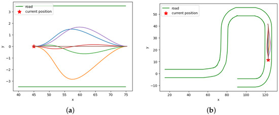
Figure 4. Example of hard exploration. Hard exploration uses fully random exploration, where only the starting point and goal point are provided, and all intermediate points are randomly sampled from the GRPs. (a) GRP samples in the Frenet frame, (b) GRP samples in the Cartesian frame.

4.3.2. Soft Exploration

In soft exploration step, the agent executes the path ${\tau }_{\pi }$ generated by the policy $\pi$ for exploration. The ratio of soft exploration increases over the episode. During execution, the agent follows each trajectory and records the s and $p_{agent}$ at each time step t. $\tau$ represents the sequence of the recorded $p_{agent}$. We will define the set of $\tau$ as $\mathcal{T}$. After all executions are completed, rewards are computed for each $\tau$. In contrast to hard exploration, soft exploration follows the points calculated from the next actions generated by the network policy.

4.3.3. Policy Update

We model our policy, which maps a state to the next K actions, as a multi-layer perceptron (MLP) as shown in Figure 5. We utilize the cross-entropy method [40] to train a $\theta$ that maximizes $R(s,{\tau }_{\pi })$. The cross-entropy method trains the elite-set, which consists of actions with the top k% rewards. In RLTF, we will refer to elite-set as ${\mathcal{T}}_{top}$. To train in the Frenet frame, ${\mathcal{T}}_{top}$ is transformed into the Frenet frame. The transformed $\tau$ is sliced into $\left|\tau \right|-K$ segments, where $\left|\tau \right|$ is the number of points in $\tau$. In the current step h, $a_h=\{p_{\tau }(h+1)-p_{\tau }\left(h\right),\dots ,p_{\tau }(h+k)-p_{\tau }(h+k-1)\}$, where $p_{\tau }(h+1)-p_{\tau }\left(h\right)$ represents the difference between the current step and next step. $s_h$ and $a_h$ are stored in $D_z$, where z is the number of obstacle vehicles in the current episode.

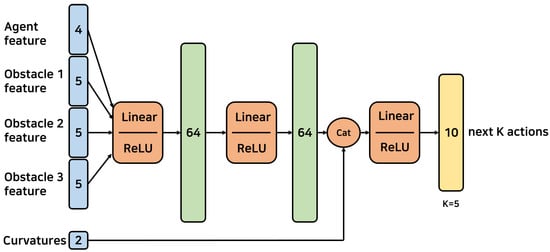
Figure 5. Multi-layer perceptron (MLP) architecture. This figure illustrates the architecture of an MLP used for our algorithm. The input layer consists of 16 neurons, representing the state space of the vehicle. This is followed by two hidden layers with 64 neurons each, using ReLU activation functions. Two curvatures are concatenated to the hidden units before passing through a final linear layer with ReLU activation, resulting in 10 output neurons representing the next $K=5$ actions.

The parameter of policy $\theta$ is updated to minimize $\ell 2$ loss at intervals when $\left|\mathcal{D}\right|$ exceeds the batch size, where $\left|\mathcal{D}\right|$ is the number of transitions in the ${\mathcal{D}}_z$ with the smallest number of transitions among all ${\mathcal{D}}_z$. AdapOptimizer with learning rate $1e^{-3}$ is employed as our optimizer. To consider all scenarios involving obstacle vehicles, samples are taken from all ${\mathcal{D}}_z$. The proposed algorithm is summarized in Algorithm 1.

Algorithm 1  Reinforcement-learning-based trajectory learning in the Frenet frame

1: Initialize $\theta$, replay buffer $\mathcal{D}$ and step = 0 2: for every episode do 3:     Initialize all vehicles pose. 4:     if $\mathrm{rand}>0.5{\displaystyle \frac{1}{1+exp\left(\frac{-\mathrm{step}}{10}\right)}}$ then 5:         Sample N trajectories ${\tau }_{grp}$ from GRPs. 6:         Transform ${\tau }_{grp}$ to Cartesian frame. 7:         for each ${\tau }_{grp}$ do 8:            Execute n-th ${\tau }_{grp}$ and record $p_{agent}$ and s. 9:            $\mathcal{T}\leftarrow \mathcal{T}\cup \tau$ 10:         end for 11:     else 12:         Generate a trajectory ${\tau }_{\pi }$ from ${\pi }_{\theta }$. 13:         Transform ${\tau }_{\pi }$ to Cartesian frame. 14:         Execute ${\tau }_{\pi }$ and record $p_{agent}$ and s. 15:         $\mathcal{T}\leftarrow \mathcal{T}\cup \tau$ 16:     end if 17:     for each $\mathcal{T}$ do 18:         Compute the reward $R_{\tau }=r(s,\tau )$ 19:     end for 20:     ${\mathcal{T}}_{top}\leftarrow$ top $k\%$ recorded trajectories $\mathcal{T}$ 21:     Transform ${\mathcal{T}}_{top}$ to Frenet frame. 22:     for each $\tau \mathrm{in}{\mathcal{T}}_{top}$ do 23:         for h=0, …, $\left|\tau \right|-K$ do 24:            $a_h\leftarrow \{p_{\tau }(h+1)-p_{\tau }\left(h\right),\dots ,p_{\tau }(h+k)-p_{\tau }(h+k-1)\}$ 25:            ${\mathcal{D}}_i\leftarrow {\mathcal{D}}_i\cup \{s_h,a_h,R_{\tau }\}$ 26:         end for 27:     end for 28:     if episode mod interval == 0 and $\mathrm{batch}\le \left|\mathcal{D}\right|$ then 29:         step = step + 1 30:         for each ${\mathcal{D}}_z$ in $\mathcal{D}$ do 31:            sample ($s_b$, $a_b$) from ${\mathcal{D}}_z$ 32:            Update $\theta$ to minimize $\ell 2$ loss. 33:         end for 34:     end if 35: end for

5. Results

For training and evaluation, we created simulations using Gazebo and Robot Operating System (ROS). ROS is an open-source meta-operating system for robots that supports passing message between process, package management, and other functionalities. Gazebo is an open source 3D robotics simulator that provides a physics engine and rendering. We used the vehicle package provided by the data speed package and used a PID controller for speed control and trajectory tracking.

In the training phase, obstacle vehicles are placed, with a maximum of three in total, with two in front of the agent and one behind. The number of obstacle vehicles in front of the agent varies from one episode to another. The agent vehicle is randomly positioned on the training road with a heading error. Obstacle vehicles are randomly generated around the agent vehicle, positioned either to the left or right of the road. The road used for training is depicted in Figure 6a and tested on Figure 6b. The simulation ends if the agent vehicle goes off the road, collides with another vehicle, or reaches the end of the road.

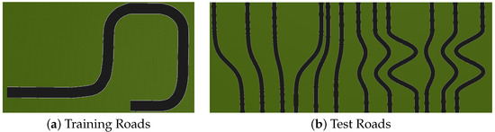
Figure 6. The roads used for (a) training and (b) tests. Test roads are not used for training.

All driving evaluations were performed on a personal desktop configured with an Intel i7-12700KF CPU and NVIDIA GeForce RTX 3080 GPU, 32GB RAM, python $3.8.10$, and pytorch $1.13.1$.

5.1. Evaluation

To demonstrate the superiority of using the Frenet frame in trajectory learning on curvy roads and the capability of RLTF to overcome drawbacks of the Frenet frame, we implemented and tested two baseline methods: RLTF without road information, which does not include lengths of obstacle vehicles and curvatures of road in the state, and RLTF without Frenet frame, which learns trajectories without using the Frenet frame. To ensure a fair evaluation, all methods share the same reward function. The evaluation was conducted on the same road used for training, with assessments occurring every 20th episode and totaling 30 evaluations in each episode. All vehicle positions were initialized using the same method as during the training phase. The obstacle vehicles are configured with one in the rear and 0 to 2 in the front, depending on the episode.

In Figure 7a, RLTF without road information shows a learning curve that closely resembles RLTF, but RLTF achieves a collision-free state at around 1900th episode, while RLTF without road information continues to result in collisions. This illustrates that not including road information in the state cannot resolve the issues associated with the Frenet frame. RLTF without Frenet frame, on the other hand, learns trajectories in the Cartesian frame instead of the Frenet frame. In Figure 7b, it is evident that methods learning trajectories in the Frenet frame achieve efficient learning, higher average rewards, and higher success rates compared to those learned in the Cartesian frame. Notably, RLTF without road information shows a very low average success rate of $60\%$.

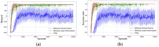
Figure 7. Average reward and success rate. (a) Average reward, (b) Average success rate.

To demonstrate that including road information resolves the issues associated with the Frenet frame, we conducted tests by fixing all state components except the road information. If road information indeed resolves Frenet frame issues, the trajectory should vary according to the road’s curvature $\kappa$; the result is in Figure 8. Positive $\kappa$ corresponds to a left curve, and negative $\kappa$ to a right curve. The increasing intensity of red indicates higher $\kappa$, while the increasing intensity of blue indicates lower $\kappa$. This demonstrates that when learning trajectories for obstacle avoidance on curved roads, using the Frenet frame for training can generate safer trajectories, and it also suggests that our state representation can address the drawbacks associated with the Frenet frame.

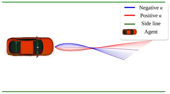
Figure 8. Comparison of trajectory variations based on curvature $\kappa$. The red color becoming darker indicates higher $\kappa$ and the blue color becoming darker indicates lower $\kappa$.

5.2. Driving Results Comparisons

To demonstrate that RLTF generates future-aware trajectories in complex scenarios, we compared it to a conventional trajectory generation (Traj. Gen.) method using the Frenet frame [19], an information-theoretic model predictive controller with neural networks (IT-MPC-NN) [29], and two other methods: supervised learning with behavior cloning (supervised BC) and reinforcement learning with behavior cloning using TD3 (TD3+BC). Supervised BC and TD3+BC have the same size of layers as RLTF, and these methods are trained to learn steering angle and throttle/brake values. All methods share the same reward function. We first conducted driving evaluations on the road used for training. All vehicle initializations were the same as in the training phase, with the number of obstacle vehicles varying from episode to episode, consisting of one in the rear and 0 to 2 in the front. Each method was evaluated for 900 episodes. The results of the comparative methods are shown in Table 3, where RLTF achieves the highest success rate, the fastest average speed, and the shortest computation time among all methods. While the other strategies did not achieve a $100\%$ success rate, RLTF achieved $100\%$ success. Figure 9 presents the driving trajectories during simulation for TD3+BC and RLTF. TD3+BC and RLTF managed to pass the first obstacle, but TD3+BC collided with the second obstacle. Additionally, it is worth noting that RLTF made earlier movements to avoid the first obstacle compared to TD3+BC. This result demonstrates that learning trajectories allow for better future planning, as RLTF exhibits a more proactive response in avoiding obstacles.

Table 3. Driving results on the training roads.

Algorithms	RLTF	IT-MPC-NN [29]	Traj. Gen. [19]	Supervised BC	TD3+BC
Average reward	424.58	414.04	401.01	234.55	325.45
Average success rate	100	100	98	80.77	90.11
Average speed	17.74	16.81	14.98	14.44	14.29
Computation time	0.458	2.29	1098.96	1.176	1.18
Average deviation	0.05	0.07	0.76	0.6	0.05
Average throttle value	0.15	0.14	0.48	0.13	0.11
Average steering angle	1.78	1.71	1.63	−1.47	−1.42
Average acceleration	0.69	0.65	0.62	0.58	0.41

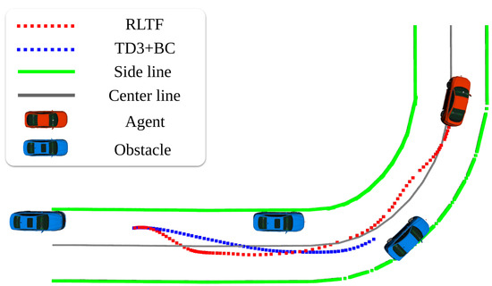
Figure 9. Simulation driving trajectory results of RLTF and TD3+BC.

We also conducted evaluations with 900 tests for each method on 12 unseen roads, as described in Table 4. The IT-MPC-NN algorithm demonstrated competitive performance on unseen roads, with a slightly lower average reward and success rate compared to RLTF but similar precision in path following. The $5\%$ failure rate of IT-MPC-NN is mainly caused by the erroneous prediction of the NN dynamic model. Unlike the previous driving results, the performance of supervised BC improved on unseen roads. However, RLTF outperformed all other methods, with a $99.6\%$ success rate. Furthermore, RLTF exhibited a lower average deviation from the road center than the other methods. A higher average deviation indicates that the vehicle deviates farther from the road center during driving.

Table 4. Driving results on unseen roads.

Algorithms	RLTF	IT-MPC-NN [29]	Supervised BC	TD3+BC
Average reward	410.2	400.3	331.48	220.5
Average success rate	99.6	95	91	79
Average speed	19.32	16.73	15.07	14.51
Average deviation	0.01	0.10	0.22	0.16
Average throttle value	0.15	0.13	0.11	0.11
Average steering angle	0.34	0.36	0.20	0.18
Average acceleration	0.85	0.71	0.46	0.48

6. Conclusions

In this paper, we proposed a reinforcement-learning-based method for learning trajectories for obstacle avoidance on curved roads with continuous obstacles. Our method overcomes the limitations of modeling real-world kinematics and distorting object shapes when generating trajectories in the Frenet frame and demonstrated a 100% success rate in the trained environment. RLTF has the limitation of requiring a reference line. However, since RLTF has demonstrated significant success in most cases, we believe it can be applied to driving in various urban environments, such as narrow city streets, when collision prevention is applied along the output trajectory.

References

- Teng, S.; Hu, X.; Deng, P.; Li, B.; Li, Y.; Ai, Y.; Yang, D.; Li, L.; Xuanyuan, Z.; Zhu, F.; et al. Motion planning for autonomous driving: The state of the art and future perspectives. IEEE Trans. Intell. Veh. 2023, 8, 3692–3711. [Google Scholar] [CrossRef]
- Maurer, M.; Gerdes, J.C.; Lenz, B.; Winner, H. Autonomous Driving: Technical, Legal and Social Aspects; Springer Nature: Berlin/Heidelberg, Germany, 2016. [Google Scholar]
- Paden, B.; Čáp, M.; Yong, S.Z.; Yershov, D.; Frazzoli, E. A survey of motion planning and control techniques for self-driving urban vehicles. IEEE Trans. Intell. Veh. 2016, 1, 33–55. [Google Scholar] [CrossRef]
- Badue, C.; Guidolini, R.; Carneiro, R.V.; Azevedo, P.; Cardoso, V.B.; Forechi, A.; Jesus, L.; Berriel, R.; Paixao, T.M.; Mutz, F.; et al. Self-driving cars: A survey. Expert Syst. Appl. 2021, 165, 113816. [Google Scholar] [CrossRef]
- Botezatu, A.P.; Burlacu, A.; Orhei, C. A Review of Deep Learning Advancements in Road Analysis for Autonomous Driving. Appl. Sci. 2024, 14, 4705. [Google Scholar] [CrossRef]
- Kuutti, S.; Bowden, R.; Jin, Y.; Barber, P.; Fallah, S. A Survey of Deep Learning Applications to Autonomous Vehicle Control. IEEE Trans. Intell. Transp. Syst. 2021, 22, 712–733. [Google Scholar] [CrossRef]
- Rausch, V.; Hansen, A.; Solowjow, E.; Liu, C.; Kreuzer, E.; Hedrick, J.K. Learning a Deep Neural Net Policy for End-to-End Control of Autonomous Vehicles. In Proceedings of the 2017 American Control Conference (ACC), Seattle, WA, USA, 24–26 May 2017; pp. 4914–4919. [Google Scholar] [CrossRef]
- Codevilla, F.; Müller, M.; López, A.; Koltun, V.; Dosovitskiy, A. End-to-end Driving via Conditional Imitation Learning. In Proceedings of the 2018 IEEE International Conference on Robotics and Automation (ICRA), Brisbane, Australia, 21–25 May 2018. [Google Scholar] [CrossRef]
- Li, Y.; Zhu, Z.; Li, X. Reinforcement Learning Based Speed Control with Creep Rate Constraints for Autonomous Driving of Mining Electric Locomotives. Appl. Sci. 2024, 14, 4499. [Google Scholar] [CrossRef]
- Tang, X.; Huang, B.; Liu, T.; Lin, X. Highway Decision-Making and Motion Planning for Autonomous Driving via Soft Actor-Critic. IEEE Trans. Veh. Technol. 2022, 71, 4706–4717. [Google Scholar] [CrossRef]
- Huang, Z.; Wu, J.; Lv, C. Efficient Deep Reinforcement Learning With Imitative Expert Priors for Autonomous Driving. IEEE Trans. Neural Netw. Learn. Syst. 2022, 34, 7391–7403. [Google Scholar] [CrossRef] [PubMed]
- Chen, Y.; Dong, C.; Palanisamy, P.; Mudalige, P.; Muelling, K.; Dolan, J.M. Attention-Based Hierarchical Deep Reinforcement Learning for Lane Change Behaviors in Autonomous Driving. In Proceedings of the IEEE/CVF Conference on Computer Vision and Pattern Recognition Workshops, Long Beach, CA, USA, 16–17 June 2019; pp. 1326–1334. [Google Scholar]
- Li, D.; Zhao, D.; Zhang, Q.; Chen, Y. Reinforcement Learning and Deep Learning based Lateral Control for Autonomous Driving. arXiv 2018, arXiv:1810.12778. [Google Scholar] [CrossRef]
- Leurent, E. A Survey of State-Action Representations for Autonomous Driving. 2018. Available online: https://hal.science/hal-01908175 (accessed on 6 August 2024).
- Li, B.; Ouyang, Y.; Li, L.; Zhang, Y. Autonomous driving on curvy roads without reliance on frenet frame: A cartesian-based trajectory planning method. IEEE Trans. Intell. Transp. Syst. 2022, 23, 15729–15741. [Google Scholar] [CrossRef]
- González, D.; Pérez, J.; Milanés, V.; Nashashibi, F. A Review of Motion Planning Techniques for Automated Vehicles. IEEE Trans. Intell. Transp. Syst. 2016, 17, 1135–1145. [Google Scholar] [CrossRef]
- LaValle, S.M.; Kuffner, J.J., Jr. Randomized kinodynamic planning. Int. J. Robot. Res. 2001, 20, 378–400. [Google Scholar] [CrossRef]
- Kavraki, L.E.; Svestka, P.; Latombe, J.C.; Overmars, M.H. Probabilistic roadmaps for path planning in high-dimensional configuration spaces. IEEE Trans. Robot. Autom. 1996, 12, 566–580. [Google Scholar] [CrossRef]
- Werling, M.; Ziegler, J.; Kammel, S.; Thrun, S. Optimal Trajectory Generation for Dynamic Street Scenarios in a Frenet Frame. In Proceedings of the 2010 IEEE International Conference on Robotics and Automation, Anchorage, AK, USA, 3–7 May 2010; IEEE: Piscataway, NJ, USA, 2010; pp. 987–993. [Google Scholar]
- Chu, K.; Lee, M.; Sunwoo, M. Local path planning for off-road autonomous driving with avoidance of static obstacles. IEEE Trans. Intell. Transp. Syst. 2012, 13, 1599–1616. [Google Scholar] [CrossRef]
- Farag, W.; Saleh, Z. Behavior Cloning for Autonomous Driving using Convolutional Neural Networks. In Proceedings of the 2018 International Conference on Innovation and Intelligence for Informatics, Computing, and Technologies (3ICT), Sakhier, Bahrain, 10–20 November 2018; pp. 1–7. [Google Scholar] [CrossRef]
- Kicki, P.; Gawron, T.; Skrzypczyński, P. A Self-Supervised Learning Approach to Rapid Path Planning for Car-Like Vehicles Maneuvering in Urban Environment. arXiv 2020, arXiv:2003.00946. [Google Scholar]
- Zhang, J.; Kong, A.; Tang, Y.; Lv, Z.; Guo, L.; Hang, P. Application of Data-Driven Model Predictive Control for Autonomous Vehicle Steering. arXiv 2024, arXiv:2407.08401. [Google Scholar] [CrossRef]
- Wang, J.; Zheng, Y.; Xu, Q.; Li, K. Data-Driven Predictive Control for Connected and Autonomous Vehicles in Mixed Traffic. In Proceedings of the American Control Conference, ACC 2022, Atlanta, GA, USA, 8–10 June 2022; IEEE: Piscataway, NJ, USA, 2022; pp. 4739–4745. [Google Scholar]
- Vu, T.M.; Moezzi, R.; Cyrus, J.; Hlava, J. Model Predictive Control for Autonomous Driving Vehicles. Electronics 2021, 10, 2593. [Google Scholar] [CrossRef]
- Chen, Z.; Lai, J.; Li, P.; Awad, O.I.; Zhu, Y. Prediction Horizon-Varying Model Predictive Control (MPC) for Autonomous Vehicle Control. Electronics 2024, 13, 1442. [Google Scholar] [CrossRef]
- Yu, S.; Sheng, E.; Zhang, Y.; Li, Y.; Chen, H.; Hao, Y. Efficient Nonlinear Model Predictive Control of Automated Vehicles. Mathematics 2022, 10, 4163. [Google Scholar] [CrossRef]
- Williams, G.; Drews, P.; Goldfain, B.; Rehg, J.M.; Theodorou, E.A. Aggressive Driving with Model Predictive Path Integral Control. In Proceedings of the 2016 IEEE International Conference on Robotics and Automation (ICRA), Stockholm, Sweden, 16–21 May 2016; pp. 1433–1440. [Google Scholar]
- Williams, G.; Drews, P.; Goldfain, B.; Rehg, J.M.; Theodorou, E.A. Information-theoretic model predictive control: Theory and applications to autonomous driving. IEEE Trans. Robot. 2018, 34, 1603–1622. [Google Scholar] [CrossRef]
- Kiran, B.R.; Sobh, I.; Talpaert, V.; Mannion, P.; Sallab, A.A.A.; Yogamani, S.; Pérez, P. Deep Reinforcement Learning for Autonomous Driving: A Survey. IEEE Trans. Intell. Transp. Syst. 2022, 23, 4909–4926. [Google Scholar] [CrossRef]
- Chen, J.; Yuan, B.; Tomizuka, M. Model-Free Deep Reinforcement Learning for Urban Autonomous Driving. In Proceedings of the 2019 IEEE Intelligent Transportation Systems Conference (ITSC), Auckland, New Zealand, 27–30 October 2019; IEEE: Piscataway, NJ, USA, 2019; pp. 2765–2771. [Google Scholar]
- Wang, P.; Li, H.; Chan, C.Y. Continuous Control for Automated Lane Change Behavior Based on Deep Deterministic Policy Gradient Algorithm. In Proceedings of the 2019 IEEE Intelligent Vehicles Symposium (IV), Paris, France, 9–12 June 2019; pp. 1454–1460. [Google Scholar] [CrossRef]
- Naveed, K.B.; Qiao, Z.; Dolan, J.M. Trajectory Planning for Autonomous Vehicles Using Hierarchical Reinforcement Learning. In Proceedings of the 2021 IEEE International Intelligent Transportation Systems Conference (ITSC), Indianapolis, IN, USA, 19–22 September 2021; IEEE: Piscataway, NJ, USA, 2021; pp. 601–606. [Google Scholar]
- Ye, L.; Zhou, Z.; Wang, J. Improving the Generalizability of Trajectory Prediction Models with Frenet-Based Domain Normalization. arXiv 2023, arXiv:2305.17965. [Google Scholar]
- Meyer, E.; Brenner, M.; Zhang, B.; Schickert, M.; Musani, B.; Althoff, M. Geometric deep learning for autonomous driving: Unlocking the power of graph neural networks with CommonRoad-Geometric. arXiv 2023, arXiv:2302.01259. [Google Scholar]
- Mirchevska, B.; Werling, M.; Boedecker, J. Optimizing trajectories for highway driving with offline reinforcement learning. Front. Future Transp. 2023, 4, 1076439. [Google Scholar] [CrossRef]
- Moghadam, M.; Alizadeh, A.; Tekin, E.; Elkaim, G.H. A Deep Reinforcement Learning Approach for Long-Term Short-Term Planning on Frenet Frame. In Proceedings of the 2021 IEEE 17th International Conference on Automation Science and Engineering (CASE), Lyon, France, 23–27 August 2021; IEEE: Piscataway, NJ, USA, 2021; pp. 1751–1756. [Google Scholar]
- Choi, S.; Lee, K.; Oh, S. Gaussian Random Paths for Real-Time Motion Planning. In Proceedings of the 2016 IEEE/RSJ International Conference on Intelligent Robots and Systems (IROS), Daejeon, Republic of Korea, 9–14 October 2016; IEEE: Piscataway, NJ, USA, 2016; pp. 1456–1461. [Google Scholar]
- Andersen, H.; Chong, Z.J.; Eng, Y.H.; Pendleton, S.; Ang, M.H. Geometric Path Tracking Algorithm for Autonomous Driving in Pedestrian Environment. In Proceedings of the 2016 IEEE International Conference on Advanced Intelligent Mechatronics (AIM), Banff, AB, Canada, 12–15 July 2016; IEEE: Piscataway, NJ, USA, 2016; pp. 1669–1674. [Google Scholar]
- Pinneri, C.; Sawant, S.; Blaes, S.; Achterhold, J.; Stueckler, J.; Rolinek, M.; Martius, G. Sample-Efficient Cross-Entropy Method for Real-Time Planning. In Proceedings of the Conference on Robot Learning, London, UK, 8–11 November 2021; PMLR. pp. 1049–1065. [Google Scholar]
Disclaimer/Publisher’s Note: The statements, opinions and data contained in all publications are solely those of the individual author(s) and contributor(s) and not of MDPI and/or the editor(s). MDPI and/or the editor(s) disclaim responsibility for any injury to people or property resulting from any ideas, methods, instructions or products referred to in the content. |
© 2024 by the authors. Licensee MDPI, Basel, Switzerland. This article is an open access article distributed under the terms and conditions of the Creative Commons Attribution (CC BY) license (https://creativecommons.org/licenses/by/4.0/).