Image Deraining Algorithm Based on Multi-Scale Features

Abstract

In target detection, tracking, and recognition tasks, high-quality images can achieve better results. However, in actual scenarios, the visual effects and data quality of images are greatly reduced due to the influence of environmental factors, which affect subsequent detection, recognition, and other tasks. Therefore, this paper proposes an image rain removal algorithm based on multi-scale features, which can effectively remove rain streaks. First of all, this paper proposes a deraining algorithm that combines spatial information to improve the network’s generalization ability on real images, aiming at the problem of synthetic datasets used by previous deraining algorithms. Then, by proposing a multi-scale rain removal algorithm, it improves the feature extraction capabilities of existing deraining algorithms. Before extracting deep rain features, a preliminary fusion of multi-scale shallow features can be performed, which can show better performance in images of different sizes. In addition, a spatial attention module and channel are introduced. The attention module increases the ability to extract rain information at each scale; the resulting multi-scale feature image rain removal algorithm is called MFD. Finally, the rain removal algorithm is validated on the rain removal dataset, and the proposed method can effectively remove rain patterns, provide strong performance improvement on several datasets in the image rain removal task, and provide high-quality images for subsequent detection and recognition tasks.

1. Introduction

In target detection, tracking, and recognition tasks, high-quality images can achieve better results. However, in actual scenarios, the visual effects and data quality of images are greatly reduced due to the influence of environmental factors, which affect subsequent detection, recognition, and other tasks. Therefore, clean background images and rain images need to be stripped from the original rain images. This is the image rain removal task.

Rain streaks can cause severe occlusion of the background scene, or rain accumulation can significantly reduce the contrast and visibility of the scene. In practical application scenarios, although the quality of rain scene images is damaged, rich content can still be extracted from them, such as the target object of the image, edge information, spatial structure, text content, semantic emotional information, etc. [1].

The innovation of new technologies has brought about ever-changing needs, which in turn has promoted the development of new technologies. The two complement each other. From research that ignores weather factors to in-depth exploration of image restoration technology, such as image rain removal, this phenomenon is favorable proof of the iterative development of image processing technology. Therefore, how to apply computer vision-related algorithms to efficiently process rain scene image data has become a difficulty that needs to be overcome in the field of computer vision, and it is also the only way for computer vision to become practical and popular [2].

Early image rain removal methods used loss functions and various prior knowledge to represent the characteristics of the rain layer and background layer [2,3,4,5,6]. Since 2017, image rain removal methods have entered the data-driven stage. In the era of deep learning, various deep learning neural networks are used to accurately extract the required rain map features to complete rain removal, such as convolutional neural network (CNN) [7,8,9], recurrent neural network (RNN) [10,11], Generative Adversarial Network (GAN) [12,13,14], semi/unsupervised learning [15,16,17], etc., these methods have demonstrated excellent performance. However, the biggest problem currently encountered by data-driven deep-learning rain removal methods is that the trained network generally has poor rain removal performance and weak generalization performance in real scenarios. First of all, existing research does not have a completely real training dataset because it cannot capture images with both rain and no rain at the same time. Therefore, the images and scene information of the same scene at different times are also different and cannot be used as a perfect comparison reference. Secondly, the current synthetic rain dataset is generally based on the physical modeling of rain, and it is difficult for the physical model to take into account all rain characteristics. Therefore, the training dataset has a certain bias, which leads to the problem of rain removal based on deep learning. The performance of the method will be greatly reduced or even useless.

Current image deraining techniques face several challenges:

(1)

Diversity of rain. Influenced by a variety of factors such as shape, size, and wind speed, rainwater has a variety of forms and characteristics. If the actual rain features are not consistent with the model presets, the effectiveness of this model will be affected.

(2)

Pairs of images with and without rain are difficult to obtain. Existing models are effective on synthetic datasets, but it is difficult to take paired no-rain and rain images in the real world, and the synthetic rain images are still different compared to the real rain images.

(3)

The generalization ability of the model needs to be improved. Currently, synthetic rain images are mainly used to train and evaluate the model, however, there are differences between synthetic rain images and real rain images. This may not be effective when dealing with irregular or dense rain in natural environments.

In view of these challenges, this paper proposes a multi-scale feature-based image deraining algorithm, which not only improves the deraining effect but also enhances the generalization of the model when dealing with rain maps for various situations.

2. Related Work

This article mainly studies image rain removal technology based on deep learning methods. Therefore, we will introduce the current research status of rain removal algorithms and focus on the image rain removal technology based on deep learning methods.

2.1. Model-Based Rain Removal Method

The model-driven rain-removal-based approach uses advanced algorithmic techniques and physical models to process and remove raindrops from images. The core of this approach lies in the construction of a model that can simulate the process of rain formation in an image and through which a clean background of the image can be separated and recovered. Traditional model-based methods still have far-reaching significance and huge reference value for current rain removal research. Therefore, the current research status of traditional model-based image rain removal algorithms will be introduced below.

As early as 2004, Garg and Nayar [3,4] began research on rain removal from video images. Kang et al. [5], as the leader in the field of single-image rain removal, extracted the high-frequency layer of the rain image in 2012 and used dictionary learning and sparse coding technology to further decompose it into rain components and non-rain components. In 2015, Luo et al. [6] proposed a learning dictionary that learns both the rain layer and the background layer. In 2016, Li et al. [18] proposed a method based on the Gaussian mixture model applied to both the background layer and the rain pattern layer to adapt to various background appearances and the appearance of rain patterns. In 2017, Zhu et al. [19] used joint optimization to alternately remove rain details from the background layer and remove non-rain details from the rain layer.

The model-based single-image rain removal method uses a large amount of physical prior knowledge as the basis, and physical modeling requires a large amount of comprehensive knowledge; there are many factors to consider, so it is difficult to cover everything. Its rain-removal effect has been proven through practice. It is highly dependent on the reliability and accuracy of the established model and cannot be widely used in the real world. The generalization performance still needs to be improved. Therefore, it is difficult to use traditional physical models to remove rain. However, rain removal methods based on prior knowledge still have a profound impact on current research and provide inspiration for current rain removal methods [20].

2.2. Rain Removal Method Based on Supervised Learning

As early as 2013, Eigen [21] et al. built a three-layer convolutional neural network to learn the mapping between damaged image patches and clear image patches. Although its network structure is simple, it provides inspiration for subsequent image rain removal algorithms based on deep learning methods. In view of the rapid development of deep learning technology, some scholars have begun to apply deep learning to the research of image rain removal algorithms. Since 2017, image rain removal technology based on deep learning (mainly supervised learning) has sprung up. In 2017, Yang et al. [22] built a multi-task architecture to learn binary rainline images, rain appearance, and clear background images. In 2017, Fu et al. [23,24] designed a deep detail network taking high-frequency details as input to predict the residual between the input image and the real image. It is worth noting that the input of high-frequency details is an important exploration of the combination of deep learning and prior knowledge. However, a key problem with early methods based on deep learning is the poor rain removal performance of the network.

With the emergence of various variants of convolutional neural networks, research on image rain removal algorithms based on convolutional neural networks has become increasingly mature. Li et al. [25] built an autoencoder network with non-locally enhanced dense blocks, where the weight values of the non-local feature maps change following four densely connected convolutional layers. Fan et al. [26] use the residuals generated by shallow image blocks to guide deep image blocks, predict negative residuals from coarse to fine, and finally fuse the outputs of different blocks. This method is an important attempt to achieve multi-scale feature fusion in the field of rain removal from a single image. Shallow features guide deep features to achieve rain removal operations from coarse to fine.

An important part of supervised learning is labeled datasets. Image rain removal methods based on supervised learning mostly use synthetic datasets. Therefore, the synthesis of rainwater datasets has also attracted the interest of researchers. Hu et al. [27] created a RainCityscapes dataset related to scene depth. At the same time, they proposed an attention mechanism based on depth guidance and built a deep network to predict residual images; coincidentally, Wang et al. [28] also constructed a high-quality dataset, including 29,500 pairs of real rain images and pseudo-real rain images. Then, they designed a new spatial attention network to effectively learn rain removal discrimination from local to global features. The creation of new datasets provides a basic data guarantee for subsequent research on rain removal algorithms and creates new possibilities for the development of rain removal algorithms.

Research on image rain removal algorithms based on convolutional neural networks is no longer satisfied with a single scale and network architecture and has begun to integrate multi-scale content and multi-layer networks. The network proposed by Fu et al. [11] combines the methods of Gaussian–Laplacian image pyramid decomposition and deep neural networks, using recursive and residual network structures to aggregate features of different layers. The introduction of the Gaussian–Laplacian image pyramid in this method not only realizes the lightweight of the rain removal network but also fully extracts the features of the multi-scale rain image to complete the subsequent rain removal operation. It is a combination of prior knowledge and knowledge in the field of single-image rain removal. Another successful case of the integration of supervised learning methods.

Wang et al. [29] proposed a multi-subnetwork structure that can learn features at different scales. These subnetworks are integrated into internal learning in a cross-scale manner by gated recurrent units and make full use of these subnetworks at different scales. This method is different from previous multi-scale methods in that it explores and verifies internal scale connection methods to improve rain removal performance. Jiang et al. [30] proposed a framework called Multi-Scale Progressive Fusion Network (MSPFN) to eliminate rainlines in a single image. This method uses recursive calculations to capture global texture for similar rainlines at different locations. This allows complementary and redundant information to be explored in the spatial dimension to characterize the target rainline. At the same time, a multi-scale pyramid structure is constructed, and an attention mechanism is further introduced to guide the fine fusion of this relevant information from different scales. The method of collaboratively representing rainlines at different scales has inspired new research ideas in the field of rain removal.

Deng et al. [31] proposed an end-to-end detail recovery rain removal network, which introduced two parallel sub-networks with comprehensive loss functions, which cooperated to eliminate rainlines and restore the lost information caused by rainline removal. detail. The detail restoration branch of the detail restoration framework is also separable. This method divides and conquers the characteristics of different tasks and provides a new idea for parallel rain removal networks. Wang et al. [32] proposed a new network architecture by setting the output residual of the network’s inherent rain structure. The structural residual setting ensures that the rain layer extracted by the network accurately conforms to the general rainline test knowledge. Such a general regularization method will naturally achieve better accuracy and generalization capabilities. Jiang et al. [33] constructed a multi-level memory compensation network (MLMCN) for rain removal, which decomposes the learning task into several sub-problems. They designed a memory compensation block (MCB) to accurately estimate rainfall information and texture. The method works well on synthetic datasets and inspires research on processing multi-scale inputs with targeted modules.

However, rainwater comes in a variety of forms and characteristics due to a number of factors such as shape, size, and wind speed. If the actual rain features do not match the model’s preset ones, the effectiveness of the model will be affected. Pairs of images with and without rain are difficult to obtain. Existing models are effective on synthetic datasets, but it is difficult to take paired no-rain and rain images in the real world, and there are still differences between synthetic rain maps compared to real rain maps. The generalization ability of the models needs to be improved. Currently, synthetic rain images are mainly used to train and evaluate the model; however, there are differences between synthetic rain images and real rain images. This may not be effective when dealing with irregular or dense rain in natural environments.

We propose a multi-scale feature-based image rain removal architecture, called MFD, which contains several key components. (1) A multi-scale feature extraction network is designed to enhance the sensory field of the model by extracting multi-scale feature information of rainwater images, and then effectively extract rainwater features of various sizes and orientations. (2) Use the channel attention module to focus on extracting feature information from each channel, then use the spatial attention module to enhance the extracted spatial information features. (3) Add horizontal connections between feature processing blocks to avoid any information loss.

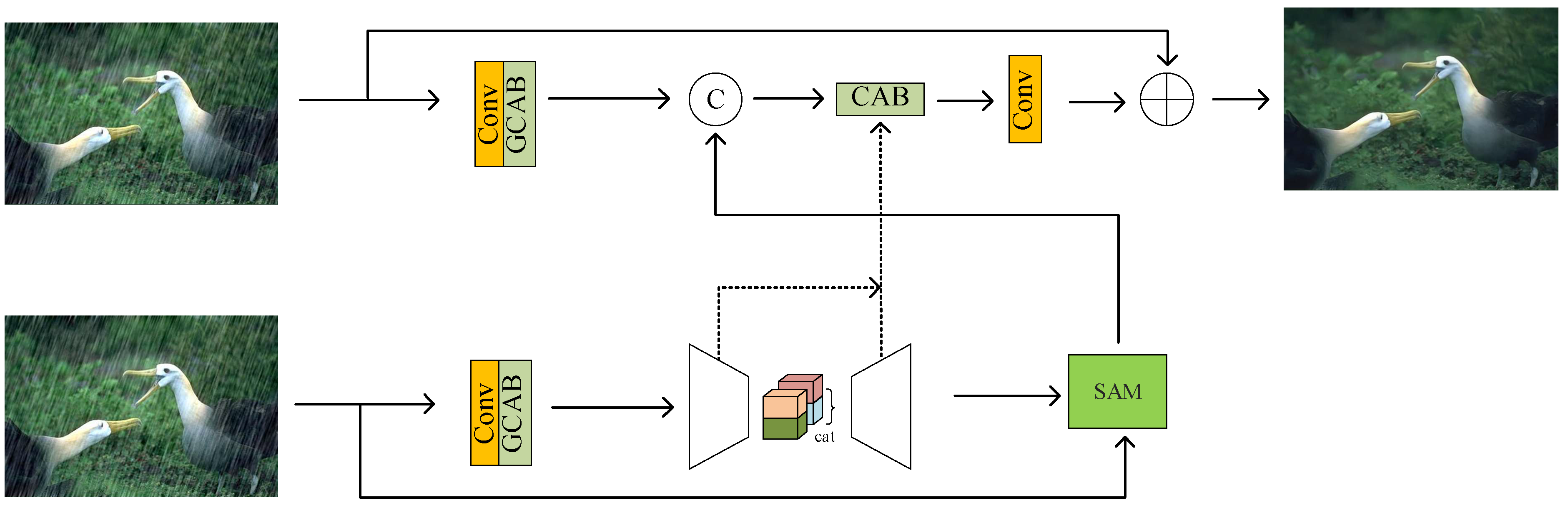
3. Multi-Scale Features to Remove Rain

The model we propose is shown in Figure 1. Firstly, it learns image features through a layer of convolution and enhances the features by a spatial attention mechanism, then it passes through an encoder–decoder network. Secondly, this network learns a wide range of contexts due to its large receptive field information. It enhances the extracted spatial features through the spatial attention module and retains the required fine features in the final output image. In order to avoid any information loss, we perform multi-scale fusion in the feature processing blocks and add lateral connections between feature processing blocks.

Figure 1. Model structure: The image features are first learned through a layer of convolution, then the features are enhanced through a spatial attention mechanism, then through an encoder–decoder network, and finally, the extracted spatial features are enhanced through a spatial attention module so that the desired fine features are preserved in the final output image.

The encoder–decoder model predicts the residual image and the final restored image is the sum of the input image and the residual image: $XS=I+RS$. We optimize our model using the following loss function:

$$L=L_{\mathrm{c}har}(X_S,Y)+\lambda L_{edge}(X_S,Y)$$

(1)

Y represents the ground truth image, L_char is the Charbonnier loss:

$$L_{char}=\sqrt{{‖X_S-Y‖}^2+{\epsilon }^2}$$

(2)

The constant ε is empirically set to 10⁻³. Furthermore, Ledge is the edge loss, defined as:

$$L_{edge}=\sqrt{{‖\Delta (X_S)-\Delta (Y)‖}^2+{\epsilon }^2}$$

(3)

where $\Delta$ represents the Laplacian operator, λ in Equation (1) and controls the relative importance of the two loss terms, as shown in [30], which is set to 0.05.

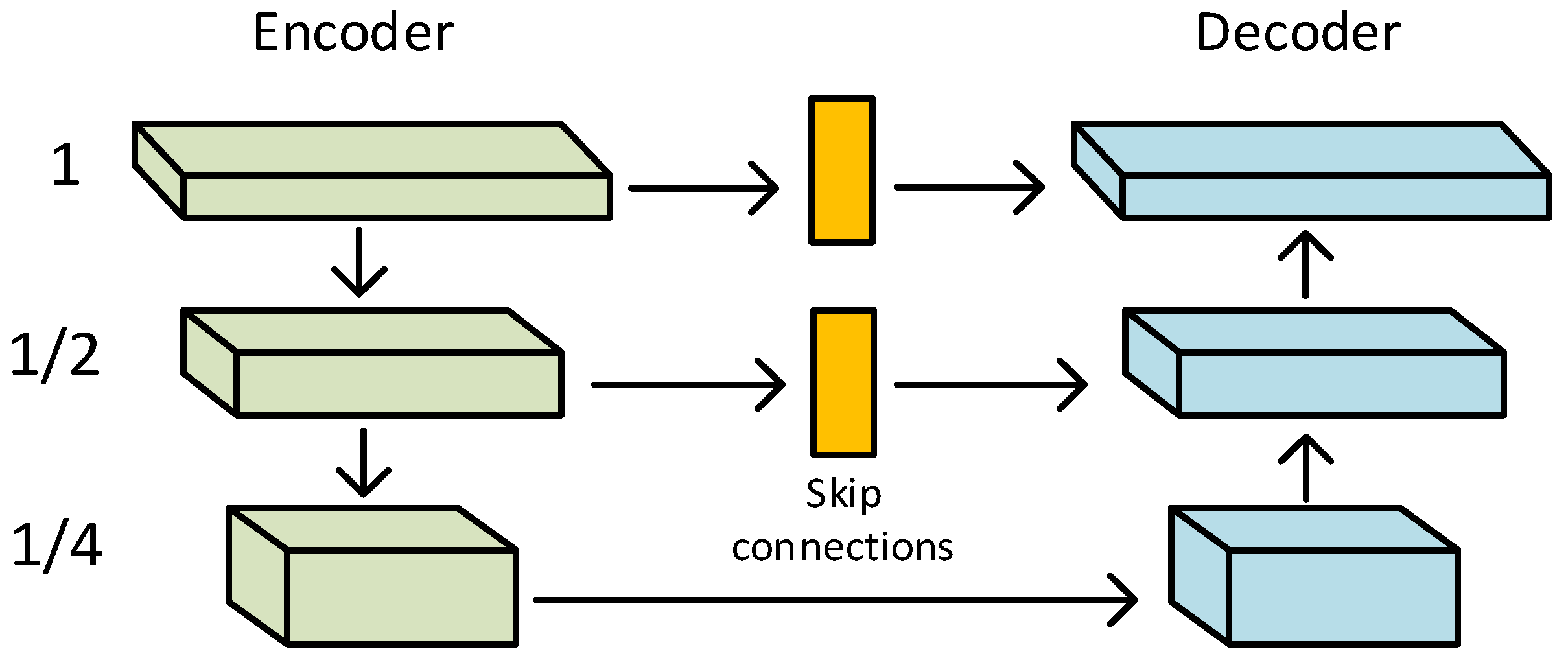
3.1. Multi-Scale Feature Processing

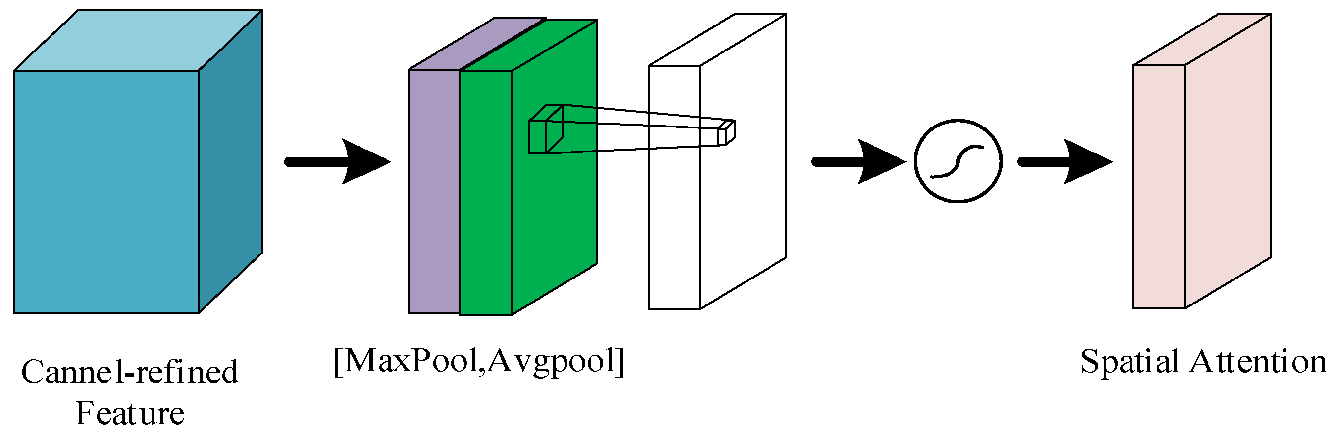
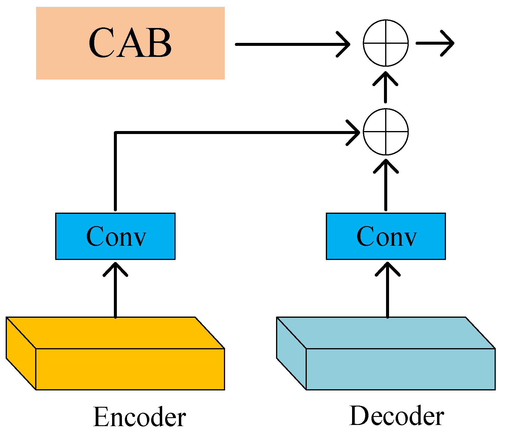
In this section, the improved U-Net network is used for multi-scale feature extraction. The structure of the U-Net model is completely different from CNN and FCN because it downsamples on its left half and upsamples reciprocally on its right half. It mainly consists of the encoder; the decoder is connected with the U-Net-style jumps. The encoder presents a structure that shrinks gradually. It reduces the resolution of the feature map constantly and then uses two convolutional layers to extract features. The decoder presents an expanding structure symmetrical to the encoder. To achieve accurate localization, it repairs the details and spatial dimensions of the segmented objects. The U-Net-style jump connection is a splicing fusion in the channel dimensions, and the jump connection is designed to make the feature map recovered from the upsampling contain more low-level semantic information. Finally, the result is more refined.

The decoder–encoder network is shown in Figure 2. It is based on the standard U-Net with the following parts. Firstly, the channel attention module is used to extract features at each scale. Secondly, the feature maps at the U-Net jump junctions are co-processed with the CAB (Channel Attention Block). Finally, bilinear interpolation upsampling and convolutional layers are used to improve the feature space resolution of the decoder instead of using transposed convolution. This approach reduces possible image artifacts caused by transposed convolution and improves the quality of the output images [34].

Figure 2. Encoder–decoder network: Firstly, the channel attention module is used to extract features at each scale; next, the feature maps at the U-Net jump junctions are co-processed with the CAB; and finally, bilinear interpolation upsampling and convolutional layers are used to improve the feature space resolution of the decoder instead of using transposed convolution.

The spatial attention module can preserve the fine details from the input image to the output image, as shown in Figure 3. Firstly, the input feature map is subjected to maximum pooling and average pooling. Then, the results of maximum pooling and average pooling are spliced according to the channels. Finally, the spliced results are subjected to the convolution operation and then processed by the activation function to obtain the feature map outputted by the spatial attention mechanism; this suppresses the less informative features and enhances the extracted spatial features.

Figure 3. Spatial attention module: Firstly, the input feature maps are subjected to maximum pooling and average pooling. Then, the results of maximum pooling and average pooling are spliced according to the channels. Finally, the spliced results are subjected to the convolution operation and then processed by the activation function to obtain the feature maps output from the spatial attention mechanism.

3.2. Feature Fusion

Feature fusion is an important method in the field of pattern recognition. The image recognition problem in the field of computer vision is a special pattern classification problem.

Feature fusion is divided into early fusion and late fusion, to alleviate the problem of inconsistency between the raw data in each modality, a representation of the features can be extracted from each modality separately and then fused at the feature level, i.e., feature fusion. Both data level and feature level fusion are referred to as early fusion since deep learning involves learning specific representations of features from the raw data, which leads to the need for data fusion sometimes before features have been extracted. Late fusion methods, also known as decision-level fusion methods, first train different modalities with different models and then fuse the outputs of multiple models. Late fusion methods mainly use rules to determine the combining strategy for different model outputs, such as maximum value combining, mean value combining, Bayesian rule combining, and integrative learning combining methods.

Early fusion is the best option with model knowledge given that both early and late fusion degrade due to a finite training set. This degradation is shown to be greater for early fusion due to the dimensionality increase in the feature space, so, eventually, late fusion could be a better option in a practical setting [35,36,37,38].

Fusing features at an early stage in the rain removal task preserves more original information, which helps the model to better learn and recover the details of the image. Additionally, different features may contain complementary information. For example, some features may be good at capturing texture, while others may be better at capturing shape. Fusing these features can help the model understand the image content more fully. The rain removal task relies more on low-level texture and edge information, which is more easily captured in the early stages. Late-stage fusion may not provide enough low-level features to effectively remove raindrops. Therefore, a module for early feature fusion is used in this paper.

In our model, as shown in Figure 4, the Cross-Stage Feature Fusion (CSFF) module is introduced between the encoder and decoder. CSFF decreases the network’s information loss caused by repeated upsampling and downsampling operations in the encoder–decoder. In addition, features can be enriched. CSFF simplifies the information flow and makes the network optimization process more stable. Figure 5 shows the Channel Attention Block (CAB).

Figure 4. CSFF block: The CSFF module is mainly used for feature fusion and feature enhancement at each feature scale. By using the CSFF module, the contextual information of the features is merged for better feature extraction of the target.

Figure 5. Channel attention block: Each channel of the feature map is treated as a feature detector, so the channel features focus on useful information in the image.

4. Experiments and Results Analysis

4.1. Datasets and Evaluation Metrics

Models were trained using 14,200 paired clean–rain images collected from multiple datasets as shown in Table 1. Models trained using these datasets were evaluated against various test sets, including the datasets in [18], Rain100H [22], Rain100L [22], Test100 [39], Test2800 [23] and Test1200 [40]. Running on Pycharm (https://www.jetbrains.com/pycharm/, accessed on 22 June 2024) with an RTX 3060 GPU (NVIDIA, Santa Clara, CA, USA) and a Ryzen 7 CPU (AMD, Santa Clara, CA, USA).

Table 1. The datasets used for training and testing.

Dataset	Rain14000	Rain800	Rain100H	Rain100L	Rain1200
Train Samples	13,500	700	0	0	0
Test Samples	500	100	100	100	400
Testset Rename	Test500	Test100	Rain100H	Rain100L	Test400

Evaluation metrics are quantitatively compared using PSNR (Peak Signal-to-Noise Ratio) and SSIM (Structural Similarity Index Measure) [41].

PSNR is the Peak Signal to Noise Ratio which reflects the ratio of the maximum power of the signal to the noise power of the signal and is often used to assess the quality of a compressed, reconstructed image. In an image, each pixel has a specific value and these color values may change during compression and decompression. Because of the wide dynamic range of the signal, PSNR is usually expressed in decibels.

PSNR is used as an objective metric for assessing image quality. However, according to numerous experimental data, PSNR scores do not always correspond exactly to the quality of images as perceived by human vision. Sometimes, images with higher PSNR are visually worse than those with lower PSNR because the perception of the human visual system to errors is not absolute. Its results are affected by many factors, for example, the human visual system perceives contrast changes at low spatial frequencies more clearly and perceives luminance changes more acutely than chromaticity changes. In addition, the perception of the human visual system to specific regions is affected by the environment, and it produces the effect of visual deception in some specific environments.

Typical peak signal-to-noise ratio values in images and video compression are between 30 dB and 50 dB. The common benchmark is 30 dB. Image degradation below 30 dB is more obvious.

Given a clean image I and a noisy image K of size m × n. The mean square error (MSE) is defined as:

$$MSE=\frac{1}{mn}{\displaystyle \sum _{i=0}^{m-1}{\displaystyle \sum _{i=0}^{n-1}{[I(i,j)-K(i,j)]}^2}}$$

(4)

PSNR (dB) is defined as:

$$PSNR=10\times {\log }_{10}(\frac{MA{X}_I^2}{MSE})$$

(5)

where MAX_I is the maximum possible pixel value of the image. If each pixel was represented by an 8-bit binary, that would be 255.

SSIM measures structural similarity which generally gives values from within a range; the larger the value, the better the quality. SSIM is a metric that measures the similarity of two images. The metric was first proposed by the Image and Video Engineering Laboratory at the University of Texas at Austin. If the two images are a derained image and a labeled image, then SSIM can be used to assess the quality of the derained image.

The SSIM formula is based on three comparative measures between samples x and y: lightness, contrast, and structure.

Lightness:

$$l(x,y)=\frac{2\times {\mu }_x\times {\mu }_y+c_1}{{\mu }_x^2+{\mu }_y^2+c_1}$$

(6)

Contrast:

$$c(x,y)=\frac{2\times {\sigma }_x\times {\sigma }_y+c_2}{{\sigma }_x^2+{\sigma }_y^2+c_2}$$

(7)

Structure:

$$s(x,y)=\frac{{\sigma }_{xy}+c_3}{{\sigma }_x\times {\sigma }_y+c_3}$$

(8)

Generally, $c_3=c_2/2$, where ${\mu }_x$ represents the mean of x, ${\mu }_y$ represents the mean of y, ${\sigma }_x^2$ represents the variance of x, ${\sigma }_y^2$ represents the variance of y, ${\sigma }_{xy}$ represents the covariance of x and y. $c_1$ and $c_2$ represent two constants in order to avoid division by 0, where $c_1={(k_1\times L)}^2$ and $c_2={(k_2\times L)}^2$. l is the range of pixel values, which is usually 255. $k_1=0.01$, $k_2=0.03$ and are all default values.

Thus:

$$SSIM(x,y)=[l{(x,y)}^{\alpha }\times c{(x,y)}^{\beta }\times s{(x,y)}^{\gamma }]$$

(9)

By setting $\alpha ,\beta ,\gamma$ to 1, we can get:

$$SSIM(x,y)=\frac{(2\times {\mu }_x\times {\mu }_y+c_1)\times (2\times {\sigma }_{xy}+c_2)}{({\mu }_x^2+{\mu }_y^2+c_1)\times ({\sigma }_x^2+{\sigma }_y^2+c_2)}$$

(10)

During each calculation, an n × n window is taken from the picture. Then, the window is continuously slid for calculation. Finally, the average value is taken as the global SSIM.

4.2. Experiment Details

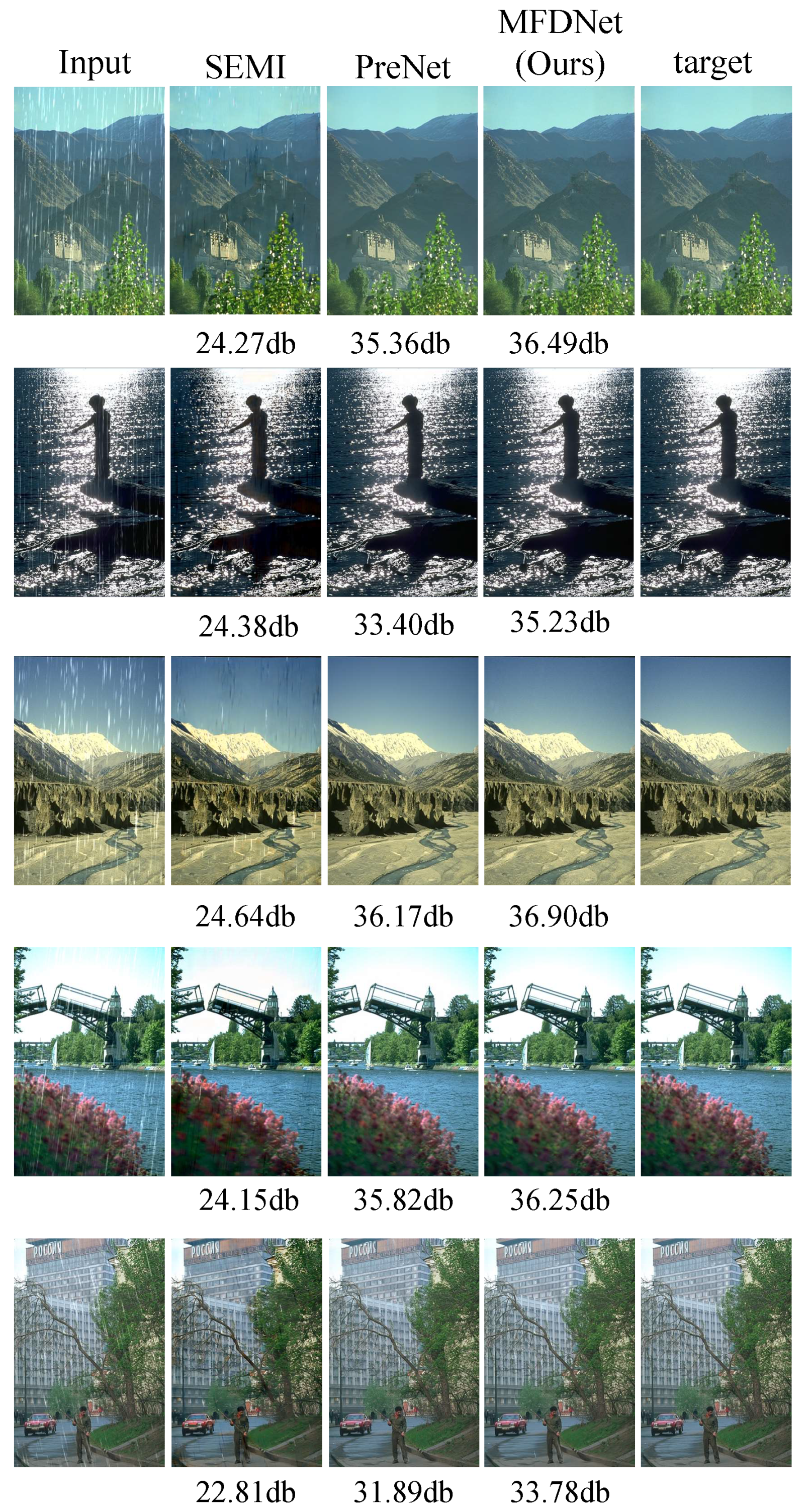
Use 2 CABs at each scale in the encoder–decoder, and for downsampling, use 2 × 2 max pooling with stride 2. When using the Adam optimizer [42], the initial learning rate is 2 × 10⁻⁴, which is steadily reduced to 1 × 10⁻⁶ using the cosine annealing strategy [43].

4.3. Derain Results

Table 2 shows that our method achieves better PSNR/SSIM scores on all 5 datasets, significantly improving the technical level. Compared to MSPFN, we obtained a performance gain of 0.986 dB.

Table 2. Image deraining results.

Method	Test100		Rain100H		Rain100L		Test400		Test500
	PSNR	SSIM	PSNR	SSIM	PSNR	SSIM	PSNR	SSIM	PSNR	SSIM
DerainNets	22.77	0.810	14.92	0.592	27.03	0.884	20.35	0.757	22.35	0.831
SEMI	22.35	0.788	16.56	0.486	25.03	0.842	20.52	0.735	25.13	0.816
DIDMDN	22.56	0.818	17.35	0.524	25.23	0.741	24.21	0.765	28.73	0.895
UMRL	24.41	0.829	26.01	0.832	29.18	0.923	25.78	0.807	29.62	0.904
RESCAN	25.00	0.835	26.36	0.786	29.80	0.881	27.44	0.810	29.51	0.877
PreNet	24.81	0.851	26.77	0.858	32.44	0.950	27.67	0.822	30.46	0.906
MSPFN	27.50	0.876	28.66	0.860	32,40	0.933	28.26	0.827	31.17	0.915
MFD (Ours)	29.45	0.874	28.67	0.870	35.01	0.959	28.12	0.839	31.67	0.919

Figure 6 shows a visual comparison of challenging images. Our model can effectively remove rain streaks of different directions and sizes and generate images that tend to be realistic. It can be seen that the SEMI method still leaves some rain patterns, the PreNet method damages the structural content and fails to restore the region obscured by rain patterns, our model can effectively remove the rain patterns and produce an image that tends to be realistic.

Figure 6. Image deraining results.

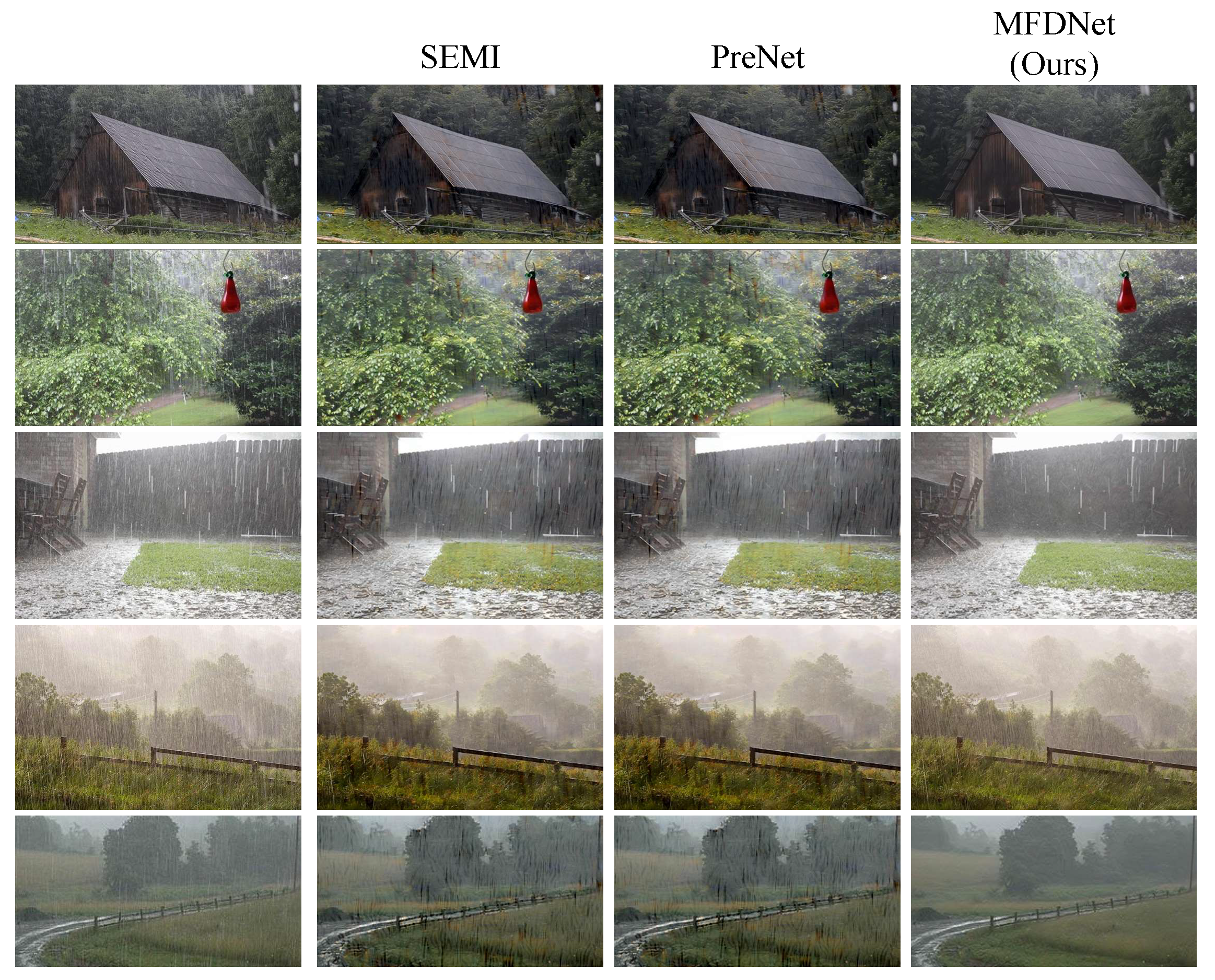
4.4. Rain Removal Experiment on a Real Rain Map

In order to verify the performance of the rain removal method proposed in this chapter when processing real rain images, this section uses the Rain100L dataset to train weights and uses the non-reference image quality evaluation indicators NIQE, BRISQUE, CEIQ, and SSEQ for evaluation, and expresses the evaluation indicators in the form of numerical values. Among them, the lower the NIQE and BRISUQE data results, the better the performance, while the larger the values of CEIQ and SSEQ, the better the performance of the corresponding method.

In a real rainy environment, it is often impossible to obtain a clear image without rain corresponding to the rainy image, so the non-reference image quality evaluation method can be used to evaluate the processed image quality. Commonly used evaluation indicators include natural image quality evaluator (NIQE), blind/referenceless image spatial quality evaluator (BRISQUE), contrast enhancement-based no-reference image quality evaluation of contrast-distorted images using contrast enhancement (CEIQ), and spatial-spectral entropy-based quality (SSEQ).

Figure 7 is the rain removal result of a real rain image and Table 3 is the performance indicators of the three algorithms on real rain maps. The SEMI method and PreNet method cannot completely remove rain streaks, they change the color of the image and introduce artifacts. The advantage of our method is that it does not introduce artifacts and can better maintain the original appearance.

Figure 7. Real rain map to remove rain results.

Table 3. Real rain map rain removal results: The performance indicators of the three algorithms on real rain maps.

Method	NIQE	BRISQUE	CEIQ	SSEQ
SEMI	19.969	28.748	4.864	2.053
PreNet	17.326	25.777	5.423	2.234
MFD (Ours)	15.422	25.094	5.463	2.549

4.5. Ablation Experiment

In order to explore the impact of different modules on rain removal performance, the following experiments were designed: Baseline is an experiment with only encoder–decoder; Baseline plus an experiment with SAM; Baseline plus an experiment with CSFF; Baseline plus an experiment with SAM and CSFF. The above experiments were all conducted on Rain100L, and the experimental results are shown in Table 4.

Table 4. Ablation experiment.

Network	PSNR	SSIM
Baseline	31.63	0.863
Baseline+SAM	33.82	0.924
Baseline+CSFF	32.26	0.916
Baseline+SAM+CSFF	35.01	0.959

From the experimental results in Table 4, it can be concluded that the SAM module improves the PSNR performance by 2.19 dB and the SSIM performance by 0.061; the CSFF module improves the PSNR performance by 0.63 dB and the SSIM performance by 0.053; the SAM and CSFF modules improve the PSNR performance by 3.38 dB and SSIM performance by 0.096 proving the effectiveness of SAM and CSFF.

5. Conclusions

In this paper, we proposed an image rain removal algorithm based on multi-scale features. Since rainwater has different sizes and directions, its features are also diverse. Therefore, a multi-scale feature extraction network was designed to enhance the sensory field by extracting multi-scale feature information and then by extracting the rainwater features of different scales and directions. A new hybrid attention module was designed. A hybrid pooling layer was added to adjust the pooling strategy according to the needs of the task and the characteristics of the data, allowing the model to generalize and adapt better in different contexts. Due to the random nature of rain patterns, it is very difficult to remove rain while retaining the details of rain-free images, so a feature enhancement module was designed. It enhances the extraction and discrimination of depth rain features in the upsampling stage and effectively avoids misjudging the location of rainlines. Based on the experimental results on five datasets, it can be concluded that the deraining algorithm proposed in this paper achieves better results on both the experimental dataset and the real rain map.

References

1. Xiao, J.; Zhou, M.; Fu, X.; Liu, A.; Zha, Z.-J. Improving De-Raining Generalization via Neural Reorganization. In Proceedings of the 2021 IEEE/CVF International Conference on Computer Vision (ICCV), Montreal, QC, Canada, 10–17 October 2021; IEEE: New York, NY, USA, 2021; pp. 4967–4976. [Google Scholar]
2. Liu, S.; Huang, D.; Wang, Y. Receptive Field Block Net for Accurate and Fast Object Detection. In Proceedings of the European Conference on Computer Vision (ECCV), Munich, Germany, 8–14 September 2018; IEEE: New York, NY, USA, 2018; pp. 404–419. [Google Scholar]
3. Garg, K.; Nayar, S.K. Detection and Removal of Rain from Videos. In Proceedings of the IEEE/CVF Conference on Computer Vision and Pattern Recognition (CVPR), Columbus, OH, USA, 23–28 June 2014; IEEE: New York, NY, USA, 2004; pp. 528–535. [Google Scholar]
4. Garg, K.; Nayar, S.K. Vision and Rain. Int. J. Comput. Vis. 2007, 75, 3–27. [Google Scholar] [CrossRef]
5. Kang, L.; Lin, C.W.; Fu, Y.H. Automatic Single-Image-Based Rain Streaks Removal via Image Decomposition. IEEE Trans. Image Process. 2011, 21, 1742–1755. [Google Scholar] [CrossRef] [PubMed]
6. Luo, Y.; Xu, Y.; Ji, H. Removing Rain from a Single Image via Discriminative Sparse Coding. In Proceedings of the IEEE International Conference on Computer Vision (ICCV), Santiago, Chile, 7–13 December 2015; IEEE: New York, NY, USA, 2015; pp. 3397–3405. [Google Scholar]
7. Yasarla, R.; Patel, V.M. Uncertainty Guided Multi-Scale Residual Learning-Using a Cycle Spinning CNN for Single Image De-Raining. In Proceedings of the IEEE/CVF Conference on Computer Vision and Pattern Recognition (CVPR), Long Beach, CA, USA, 15–20 June 2019; IEEE: New York, NY, USA, 2019; pp. 8405–8414. [Google Scholar]
8. Zhou, M.; Xiao, J.; Chang, Y.; Fu, X.; Liu, A.; Pan, J.; Zha, Z.J. Image De-raining via Continual Learning. In Proceedings of the IEEE/CVF Conference on Computer Vision and Pattern Recognition (CVPR), Nashville, TN, USA, 20–25 June 2021; IEEE: New York, NY, USA, 2021; pp. 4905–4914. [Google Scholar]
9. Nanba, Y.; Miyata, H.; Han, X. Dual Heterogeneous Complementary Networks for Single Image Deraining. In Proceedings of the IEEE/CVF Conference on Computer Vision and Pattern Recognition (CVPR), New Orleans, LA, USA, 18–24 June 2022; IEEE: New York, NY, USA, 2022; pp. 567–576. [Google Scholar]
10. Li, X.; Wu, J.; Lin, Z.; Liu, H.; Zha, H. Recurrent Squeeze-and-Excitation Context Aggregation Net for Single Image Deraining. In Proceedings of the European Conference on Computer Vision (ECCV), Munich, Germany, 8–14 September 2018; IEEE: New York, NY, USA, 2018; pp. 262–277. [Google Scholar]
11. Fu, X.; Liang, B.; Huang, Y.; Ding, X.; Paisley, J. Lightweight Pyramid Networks for Image Deraining. IEEE Trans. Neural Netw. Learn. Syst. 2020, 31, 1794–1807. [Google Scholar] [CrossRef] [PubMed]
12. Wei, Y.; Zhang, Z.; Wang, Y.; Zhang, H.; Zhao, M.; Xu, M.; Wang, M. Semi-Deraingan: A New Semi-Supervised Single Image Deraining. In Proceedings of the IEEE International Conference on Multimedia and Expo (ICME), Shenzhen, China, 5–9 July 2021; IEEE: New York, NY, USA, 2021; pp. 1–6. [Google Scholar]
13. Wei, Y.; Zhang, Z.; Wang, Y.; Xu, M.; Yang, Y.; Yan, S.; Wang, M. DerainCycleGAN: Rain Attentive CycleGAN for Single Image Deraining and Rainmaking. IEEE Trans. Image Process. 2021, 30, 4788–4801. [Google Scholar] [CrossRef] [PubMed]
14. Chen, X.; Pan, J.; Jiang, K.; Li, Y.; Huang, Y.; Kong, C.; Dai, L.; Fan, Z. Unpaired Deep Image Deraining Using Dual Contrastive Learning. In Proceedings of the IEEE/CVF Conference on Computer Vision and Pattern Recognition (CVPR), New Orleans, LA, USA, 18–24 June 2022; IEEE: New York, NY, USA, 2022; pp. 2007–2016. [Google Scholar]
15. Su, Z.; Zhang, Y.; Zhang, X.P.; Qi, F. Non-local Channel Aggregation Network for Single Image Rain Removal. Neurocomputing 2022, 469, 261–272. [Google Scholar] [CrossRef]
16. Ye, Y.; Yu, C.; Chang, Y.; Zhu, L.; Zhao, X.L.; Yan, L.; Tian, Y. Unsupervised Deraining: Where Contrastive Learning Meets Self-Similarity. In Proceedings of the IEEE/CVF Conference on Computer Vision and Pattern Recognition (CVPR), New Orleans, LA, USA, 18–24 June 2022; IEEE: New York, NY, USA, 2022; pp. 5811–5820. [Google Scholar]
17. Yu, C.; Chang, Y.; Li, Y.; Zhao, X.; Yan, L. Unsupervised Image Deraining: Optimization Model Driven Deep CNN. In Proceedings of the 29th ACM International Conference on Multimedia (ACMM), Virtual, 20–24 October 2021; ACM: New York, NY, USA, 2021; pp. 2634–2642. [Google Scholar]
18. Li, Y. Rain Streak Removal Using Layer Priors. In Proceedings of the IEEE/CVF Conference on Computer Vision and Pattern Recognition (CVPR), Las Vegas, NV, USA, 27–30 June 2016; IEEE: New York, NY, USA, 2016; pp. 2736–2744. [Google Scholar]
19. Zhu, L.; Fu, C.W.; Lischinski, D.; Heng, P.A. Joint Bi-layer Optimization for Single-Image Rain Streak Removal. In Proceedings of the IEEE/CVF International Conference on Computer Vision and Pattern Recognition (CVPR), Honolulu, HI, USA, 21–26 July 2017; IEEE: New York, NY, USA, 2017; pp. 2545–2553. [Google Scholar]
20. Zhu, H.; Wang, C.; Zhang, Y.; Su, Z.; Zhao, G. Physical Model Guided Deep Image Deraining. In Proceedings of the 2020 IEEE International Conference on Multimedia and Expo (ICME), London, UK, 6–10 July 2020; pp. 1–6. [Google Scholar]
21. Eigen, D.; Krishnan, D.; Fergus, R. Restoring an Image Taken through a Window Covered with Dirt or Rain. In Proceedings of the IEEE/CVF International Conference on Computer Vision and Pattern Recognition (CVPR), Columbus, OH, USA, 23–28 June 2014; IEEE: New York, NY, USA, 2014; pp. 633–640. [Google Scholar]
22. Yang, W.; Tan, R.T.; Feng, J.; Liu, J.; Guo, Z.; Yan, S. Deep Joint Rain Detection and Removal from a Single Image. In Proceedings of the IEEE/CVF Conference on Computer Vision and Pattern Recognition (CVPR), Honolulu, HI, USA, 21–26 July 2017; IEEE: New York, NY, USA, 2017; pp. 1685–1694. [Google Scholar]
23. Fu, X.; Huang, J.; Zeng, D.; Huang, Y.; Ding, X.; Paisley, J. Removing Rain from Single Images via a Deep Detail Network. In Proceedings of the IEEE/CVF Conference on Computer Vision and Pattern Recognition (CVPR), Honolulu, HI, USA, 21–26 July 2017; IEEE: New York, NY, USA, 2017; pp. 1715–1723. [Google Scholar]
24. Fu, X.; Huang, J.; Ding, X.; Liao, Y.; Paisley, J. Clearing the Skies: A Deep Network Architecture for SingleImage Rain Removal. IEEE Trans. Image Process. 2017, 26, 2944–2956. [Google Scholar] [CrossRef]
25. Li, G.; He, X.; Zhang, W.; Chang, H.; Dong, L.; Lin, L. Non-locally Enhanced Encoder-Decoder Network for Single Image De-raining. In Proceedings of the 26th ACM International Conference on Multimedia (ACMM), Seoul, Republic of Korea, 22–26 October 2018; ACM: New York, NY, USA, 2018; pp. 1056–1064. [Google Scholar]
26. Fan, Z.; Wu, H.; Fu, X.; Huang, Y.; Ding, X. Residual-Guide Network for Single Image Deraining. In Proceedings of the 26th ACM International Conference on Multimedia (ACMM), Seoul, Republic of Korea, 22–26 October 2018; ACM: New York, NY, USA, 2018; pp. 1751–1759. [Google Scholar]
27. Hu, X.; Fu, C.W.; Zhu, L.; Heng, P.A. Depth-Attentional Features for Single-Image Rain Removal. In Proceedings of the IEEE/CVF Conference on Computer Vision and Pattern Recognition (CVPR), Long Beach, CA, USA, 15–20 June 2019; IEEE: New York, NY, USA, 2019; pp. 8022–8031. [Google Scholar]
28. Wang, T.; Yang, X.; Xu, K.; Chen, S.; Zhang, Q.; Lau, R.W. Spatial Attentive Single-Image Deraining with a High Quality Real Rain Dataset. In Proceedings of the IEEE/CVF Conference on Computer Vision and Pattern Recognition (CVPR), Long Beach, CA, USA, 15–20 June 2019; IEEE: New York, NY, USA, 2019; pp. 12270–12279. [Google Scholar]
29. Wang, C.; Xing, X.; Wu, Y.; Su, Z.; Chen, J. DCSFN: Deep Cross-Scale Fusion Network for Single Image Rain Removal. In Proceedings of the 28th ACM International Conference on Multimedia (ACMM), Seattle, WA, USA, 12–16 October 2020; ACM: New York, NY, USA, 2020; pp. 1643–1651. [Google Scholar]
30. Jiang, K.; Wang, Z.; Yi, P.; Chen, C.; Huang, B.; Luo, Y.; Ma, J.; Jiang, J. Multi-Scale Progressive Fusion Network for Single Image Deraining. In Proceedings of the IEEE/CVF Conference on Computer Vision and Pattern Recognition (CVPR), Seattle, WA, USA, 13–19 June 2020; IEEE: New York, NY, USA, 2020; pp. 8343–8352. [Google Scholar]
31. Deng, S.; Wei, M.; Wang, J.; Feng, Y.; Liang, L.; Xie, H.; Wang, F.L.; Wang, M. Detail-recovery Image Deraining via Context Aggregation Networks. In Proceedings of the IEEE/CVF Conference on Computer Vision and Pattern Recognition (CVPR), Seattle, WA, USA, 13–19 June 2020; IEEE: New York, NY, USA, 2020; pp. 14548–14557. [Google Scholar]
32. Wang, C.; Wu, Y.; Su, Z.; Chen, J. Joint Self-Attention and Scale-Aggregation for Self-Calibrated Deraining Network. In Proceedings of the 28th ACM International Conference on Multimedia (ACMM), Seattle, WA, USA, 12–16 October 2020; ACM: New York, NY, USA, 2020; pp. 2517–2525. [Google Scholar]
33. Jiang, K.; Wang, Z.; Yi, P.; Chen, C.; Wang, X.; Jiang, J.; Xiong, Z. Multi-level Memory Compensation Network for Rain Removal via Divide-and-Conquer Strategy. IEEE J. Sel. Top. Signal Process. 2021, 15, 216–228. [Google Scholar] [CrossRef]
34. Odena, A.; Dumoulin, V.; Olah, C. Deconvolution and Checkerboard Artifacts. Distill 2016, 1, e3. [Google Scholar] [CrossRef]
35. Pereira, L.M.; Salazar, A.; Vergara, L. A comparative analysis of early and late fusion for the multimodal two-class problem. IEEE Access 2023, 11, 84283–84300. [Google Scholar] [CrossRef]
36. Salazar, A.; Safont, G.; Vergara, L.; Vidal, E. Graph Regularization Methods in Soft Detector Fusion. IEEE Access 2023, 11, 144747–144759. [Google Scholar] [CrossRef]
37. Pereira, L.M.; Salazar, A.; Vergara, L. A Comparative Study on Recent Automatic Data Fusion Methods. Computers 2023, 13, 13. [Google Scholar] [CrossRef]
38. Salazar, A.; Vergara, L.; Vidal, E. A proxy learning curve for the Bayes classifier. Pattern Recognit. 2023, 136, 109240. [Google Scholar] [CrossRef]
39. Zhang, H.; Sindagi, V.; Patel, V.M. Image de-raining using a conditional generative adversarial network. IEEE Trans. Circuits Syst. Video Technol. 2019, 30, 3943–3956. [Google Scholar] [CrossRef]
40. Zhang, H.; Patel, V.M. Density-aware single image de-raining using a multi-stream dense network. In Proceedings of the IEEE Conference on Computer Vision and Pattern Recognition (CVPR), Salt Lake City, UT, USA, 18–23 June 2018. [Google Scholar]
41. Wang, Z.; Bovik, A.C.; Sheikh, H.R.; Simoncelli, E.P. Simoncelli. Image quality assessment: From error visibility to structural similarity. IEEE Trans. Image Process. 2004, 13, 600–612. [Google Scholar] [CrossRef] [PubMed]
42. Kingma, D.P.; Ba, J. Adam: A method for stochastic optimization. arXiv 2014, arXiv:1412.6980. [Google Scholar]
43. Loshchilov, I.; Hutter, F. SGDR: Stochastic gradient descent with warm restarts. arXiv 2017, arXiv:1608.03983. [Google Scholar]
Disclaimer/Publisher’s Note: The statements, opinions and data contained in all publications are solely those of the individual author(s) and contributor(s) and not of MDPI and/or the editor(s). MDPI and/or the editor(s) disclaim responsibility for any injury to people or property resulting from any ideas, methods, instructions or products referred to in the content.
Article Metrics
Citations
Article Access Statistics
Multiple requests from the same IP address are counted as one view.