Bridging Continuous and Lattice-Based Models of Two-Dimensional Diffusion: A Systematic Approach for Estimating Transition Probabilities, Grid Size and Diffusivity

Abstract

Lattice-based models have been broadly applied in mathematical and computational modeling of biological and biomedical systems for which spatial effects are important. These discrete models commonly include diffusion of mobile constituents as a key underlying mechanism. While the direct simulation of diffusion in continuous (off-lattice) domains is possible, it is computationally intensive, particularly when multiple coupled mechanisms are involved. This study presents a systematic approach for connecting continuous models of two-dimensional diffusion with internal obstacles to discrete, lattice-based (surrogate) models of diffusion. Results from continuous model simulations on a representative domain, and over many realizations, are used to develop accurate lattice-based surrogate models by exploiting internal symmetries. Probabilities determined for the lattice-based surrogate models are also connected to theoretical diffusivities for 2D random walks on a square lattice, necessitating the calibration of a spatial grid size. This approach can facilitate the inclusion of more accurate diffusive transport models of complex media within the general framework of lattice-based models that incorporate multiple coupled mechanisms.

1. Introduction

Lattice-based models have seen broad application in the study of a variety of mechanisms and dynamics through simulation in environments where incorporation of spatial effects is important. For example, they have been commonly used for modeling biotransport, cell dynamics and tissue dynamics with applications in many biological and biomedical areas [1,2,3,4,5,6]. One example is the cellular Potts model, in which a biological cell is defined over a region comprising multiple lattice sites [2,5,6]. This lattice-based modeling framework enables the study of coupled mechanisms in biological cell dynamics and has been applied to various biomedical problems, including epidermal biology, cancer, angiogenesis and vasculogenesis [1,4]. Such discrete, lattice-based models commonly involve diffusion (e.g., of mobile solutes) as a key transport mechanism. Alternatively, agent-based models [7,8,9] often restrict movement to a lattice, with random walks commonly used as a simple or convenient approach to advance individual agent locations at each time increment. In such cases, diffusion of nutrients and cell-synthesized solutes is an important coupled mechanism.

As computing power has advanced, direct simulation in continuous-domain (off-lattice) models is a useful tool for investigating systems where particles or agents interact with a background medium or with each other. However, the direct approach can become tedious or computationally intensive in situations involving several coupled mechanisms or complex geometry or in the presence of many particles or agents. The ability to systematically connect off-lattice (continuous) models to lattice-based (discrete) models, accounting for a few key underlying model features or mechanisms, has the potential to improve the overall accuracy of discrete models. Moreover, such discrete models can also be connected to estimates of theoretical diffusivities for random walks on a two-dimensional (2D) square lattice. An appropriate spatial length scale (grid size) must be determined for the discrete model, especially when diffusion is one of several coupled mechanisms in a 2D lattice-based model.

In this study, we evaluate the extent to which 2D lattice-based surrogate models can preserve measures of particle diffusivity observed in direct simulation of continuous models based on 2D random walks with internal obstacles. Our overall approach is illustrated in Figure 1. Results from continuous model simulations (Figure 1A) on a 2D representative volume element (RVE), and over many realizations, are used to develop lattice-based surrogate models (Figure 1B) that reproduce key features of the continuous model. This is accomplished by exploiting internal symmetries in the continuous model representation. Probabilities in the lattice-based surrogate models are also connected to theoretical diffusivities for 2D random walks on a square lattice (Figure 1C). This final step requires calibration of the discrete length scale (grid size) in the square lattice surrogate model.

Figure 1. Illustration of the approach used for bridging continuous and lattice-based models in this study.

The random walker is prescribed a fixed particle radius, and obstacle radii are varied in the context of two different obstacle configurations, each having distinct internal symmetries. Particle dynamics observed for the continuous model simulations are used to develop probabilistic lattice-based surrogate models for transitions across RVE subdomains. The subdomains are chosen to preserve internal symmetries for each of the two obstacle arrangements. A primary advantage of this approach is the capability of the surrogate models to bypass the need to directly represent the obstacles in the simulation domain.

The well-known linear relationship between the mean squared particle displacement and time for the continuous model [10,11,12] is used to estimate and compare diffusivities for both the continuous and lattice-based surrogate models. This comparison motivates the introduction of a simulation parameter (commitment index) that is calibrated to minimize adverse effects of noise on achieving stationarity of transition probabilities in the lattice-based surrogate model. Theoretical derivations for isotropic and anisotropic diffusion on a 2D lattice are used to connect the transition probabilities in the lattice-based surrogate models to theoretical estimates of the diffusivity for a square lattice surrogate model. Relations enforcing consistency between diffusivity estimates, based on continuous model simulations and analytical results on the lattice, are used to estimate the effective spacing (grid size) in a (square) lattice-based model for both obstacle configurations.

This paper is organized as follows. In Section 2, effective diffusivity is first outlined in terms of the mean squared displacement of a single particle undergoing a 2D random walk in a continuous domain or on a 2D lattice. Section 3 presents our equally spaced obstacles model (Section 3.2) and our multisize obstacles model (Section 3.3). Within each model, quantities are defined to determine probabilities connecting the continuous model with its lattice-based surrogate model. In Section 4, methods for calibrating the lattice-based surrogate models based on the continuous model simulation results are first presented (Section 4.1). A framework is then presented to connect the lattice-based surrogate models to square lattice surrogate models (Section 4.2), necessitating the calibration of the square lattice grid size parameter. Our results are presented for both models in Section 5, including the calculation of all model probabilities and calibration of other model parameters, followed by a brief discussion and conclusions in Section 6. Supplementary derivations are presented in Appendix A and Appendix B.

2. Effective Diffusivity

We first summarize approaches for estimating the effective diffusivity of a particle undergoing 2D random walks based on observations of its mean squared displacement.

2.1. Effective Diffusivity in a Continuous Domain

Normal diffusion describes diffusion via random walks of a particle in a continuous domain. The mean-squared displacement $⟨r^2⟩$, relative to a fixed starting location at $t=0$, is calculated by averaging displacement trajectories over a large number of realizations. In prior studies of 2D single particle random walks, it was shown that $⟨r^2⟩$ grows linearly with time (t) after a sufficiently large number of time steps have passed [10,11,12]. The general formula for normal diffusion is written in terms of an effective diffusivity ($\kappa$) as [11,12,13]

$$⟨r^2⟩=\left(2d\right)\kappa t,$$

(1)

where d is the dimension of the medium. In our study, all simulation results are sampled in a stationary time regime where this observed relationship is linear; the effective diffusivity is estimated by rearranging (1) to obtain

$$\kappa =\frac{⟨r^2⟩}{\left(2d\right)N\Delta t},$$

(2)

where N is the number of time steps (of size $\Delta t$) in the simulation.

2.2. Effective Diffusivity on a 2D Lattice

To develop our lattice-based surrogate models, we estimate the diffusivity analogous to (2) but based on analyzing $⟨r^2⟩$ on the lattice. In this section, we demonstrate, via an analytical derivation, that a particle undergoing random walks on a 2D lattice exhibits normal diffusion, to leading order. Overall, our derivations of mean squared displacements and theoretical diffusivities for random walks on 2D lattices are based on analytical approaches outlined in Holmes [14].

We can track $⟨r^2⟩$ systematically through a set of transition probabilities (Figure 2). Here, $p_x$ and $p_y$ denote the probability of moving, at the next time step, to adjacent horizontal (by $\Delta x$) or vertical (by $\Delta y$) lattice sites, respectively. The particle remains in its current location with probability $1-p_x-p_y$. In this section, we denote the mean squared displacement as $⟨r_K^2\left(N\right)⟩$, with K referring to the number of realizations of a single particle random walk on the 2D lattice and N denoting a particular time step.

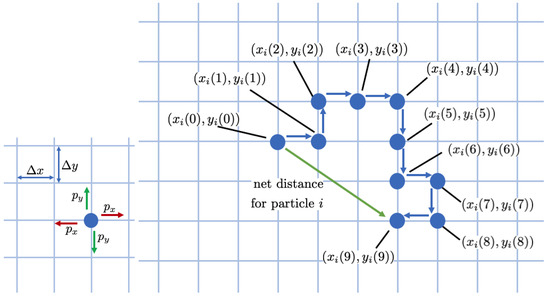
Figure 2. Illustration of a particle undergoing a random walk on a 2D lattice. The particle moves one step (size $\Delta x$) in the horizontal direction with probability $p_x$ (left) and one step (size $\Delta y$) in the vertical direction with probability $p_y$ (right). The probability of staying in place is $1-p_x-p_y$.

2.2.1. Lattice Representation of Mean Squared Displacement

The mean squared displacement after N time steps and for K realizations is

$$⟨r_K^2\left(N\right)⟩=\frac{1}{K}\sum _{i=1}^K{x}_i^2\left(N\right)+y_i^2\left(N\right),$$

(3)

where $x_i\left(N\right)$ and $y_i\left(N\right)$ are the horizontal and vertical particle locations, respectively. The mean squared displacement is then $⟨r^2⟩={lim}_{K\to \infty }⟨r_K^2\left(N\right)⟩$.

For brevity, let $x_i^N$ and $y_i^N$ denote the horizontal and vertical positions of the $i^{th}$ particle at time step N, respectively, (the full notation is utilized in the Appendices). We write these positions as

$$x_i^N=x_i^{N-1}+h_{xi}^N,y_i^N=y_i^{N-1}+h_{yi}^N,i=1,\cdots ,K,$$

(4)

where $h_{xi}^N$ and $h_{yi}^N$ are the possible displacements with associated step sizes of $\Delta x$ and $\Delta y$, respectively. In any one time step $\Delta t$, the five possible transitions are

$$\left(\mathrm{i}\right)h_{xi}^N=\pm \Delta x,h_{yi}^N=0,\left(\mathrm{ii}\right)h_{xi}^N=0,h_{yi}^N=\pm \Delta y,\left(\mathrm{iii}\right)h_{xi}^N=h_{yi}^N=0,$$

(5)

where cases (i) (horizontal transition) and (ii) (vertical transition) occur with equal probability, and case (iii) represents no transition.

Substituting (4) into (3), $⟨r^2⟩$ can be written in recursive form as

$$\begin{array}{cc}\hfill ⟨r^2⟩& =\underset{K\to \infty }{lim}⟨r_K^2\left(N\right)⟩=\underset{K\to \infty }{lim}\frac{1}{K}\sum _{i=1}^K{\left(x_i^{N-1}+h_{xi}^N\right)}^2+{\left(y_i^{N-1}+h_{yi}^N\right)}^2,\hfill \\ \hfill & =\underset{K\to \infty }{lim}\frac{1}{K}\sum _{i=1}^K\left[{\left(x_i^{N-1}\right)}^2+x_i^{N-1}{h}_{xi}^N+{\left(h_{xi}^N\right)}^2\right.\hfill \\ \hfill & +\left.{\left(y_i^{N-1}\right)}^2+y_i^{N-1}{h}_{yi}^N+{\left(h_{yi}^N\right)}^2\right],\hfill & \hfill \hspace{1em}\\ \hfill & =\underset{K\to \infty }{lim}⟨r_{K-1}^2\left(N\right)⟩\hfill & \hfill .\\ \hfill & +\underset{K\to \infty }{lim}\frac{1}{K}\sum _{i=1}^K\left[x_i^{N-1}{h}_{xi}^N+{\left(h_{xi}^N\right)}^2+y_i^{N-1}{h}_{yi}^N+{\left(h_{yi}^N\right)}^2\right].\hfill & \hfill \hspace{1em}\end{array}$$

(6)

In the next subsection, we briefly discuss limits used to simplify (6).

2.2.2. Useful Limits for Simplifying Equation (6)

We use two main limit results in simplifying Equation (6). Direct evaluation of these limits is summarized in Appendix A and Appendix B, resulting in the following values associated with case (i) (horizontal transition) above:

$$\begin{array}{ccc}\hfill & \underset{K\to \infty }{lim}\frac{1}{K}\sum _{i=1}^K{\left(h_{xi}^N\right)}^2=p_x{(\Delta x)}^2,\hfill & \hfill \underset{K\to \infty }{lim}\frac{2}{K}\sum _{i=1}^K{x}_i^N{h}_{xi}^M=0\mathrm{when}M>N.\end{array}$$

(7)

Analogous results also hold for the vertical transition case (ii).

2.2.3. Reduced Form of Mean Squared Displacement

Using (7), we rewrite (6) as

$$\begin{array}{cc}\hfill \underset{K\to \infty }{lim}⟨r_K^2\left(N\right)⟩=& \underset{K\to \infty }{lim}⟨r_{K-1}^2\left(N\right)⟩+\underset{K\to \infty }{lim}\frac{1}{K}\sum _{i=1}^K{x}_i^{N-1}{h}_{xi}^N+\underset{K\to \infty }{lim}\frac{1}{K}\sum _{i=1}^K{y}_i^{N-1}{h}_{yi}^N\hfill \\ \hfill & +\underset{K\to \infty }{lim}\frac{1}{K}\sum _{i=1}^K{\left(h_{xi}^N\right)}^2+\underset{K\to \infty }{lim}\frac{1}{K}\sum _{i=1}^K{\left(h_{yi}^N\right)}^2,\hfill \end{array}$$

(8)

to simplify (8) to the relation,

$$\begin{array}{cc}\hfill \underset{K\to \infty }{lim}⟨r_K^2\left(N\right)⟩& =\underset{K\to \infty }{lim}⟨r_{K-1}^2\left(N\right)⟩+p_x{(\Delta x)}^2+p_y{(\Delta y)}^2.\hfill \end{array}$$

(9)

Lastly, the recurrence property enables (9) to be simplified to

$$\begin{array}{cc}\hfill ⟨r^2⟩=\underset{K\to \infty }{lim}⟨r_K^2\left(N\right)⟩=& N{p}_x{(\Delta x)}^2+N{p}_y{(\Delta y)}^2.\hfill \end{array}$$

(10)

On a square lattice ($\Delta x=\Delta y$), (10) can be reduced to the linear relation

$$⟨r^2⟩=\underset{K\to \infty }{lim}⟨r_K^2\left(N\right)⟩=N(p_x+p_y){(\Delta x)}^2=N(1-q){(\Delta x)}^2,$$

(11)

where we denote q as the probability of staying in the current subdomain, i.e., since $q+p_x+p_y=1$. Equation (11) will serve as the basis for connecting the square lattice surrogate models with the lattice-based surrogate models obtained from the continuous model simulations (see Section 4.3).

3. Models

We consider direct simulation of 2D random walks on a continuous domain. Results from these simulations are used to determine transition probabilities in the lattice-based surrogate model. The number of such independent probabilities, as well as their values, change for different obstacle arrangements. We consider a single particle undergoing random walks in a 2D representative volume element (RVE). Within the RVE, we place a small number of rigid obstacles with which the particle collides; the collisions are idealized to be perfectly elastic with the angle of reflection equal to the angle of incidence. The RVE is assumed to have periodic boundary conditions, further capturing internal symmetries in the background medium. Two different obstacle arrangements are considered (Figure 3): (i) equally spaced obstacles (Figure 3a) and (ii) multisize obstacles (Figure 3b). While both cases model inhomogeneous, anisotropic materials, case (i) exhibits a greater degree of (rotational) symmetry as compared to case (ii). The second case also serves as a simple analogue of a composite with two different obstacle sizes.

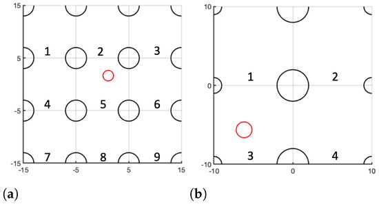
Figure 3. Sample domains (RVEs) for continuous model simulations ($R_{\mathrm{part}}=1.0$), with numbered subdomains: (a) equally spaced obstacles model (with $R_{\mathrm{obs}}=2.0$); (b) multisize obstacles model (with $R_{{\mathrm{obs}}_1}=1.0$ and $R_{{\mathrm{obs}}_2}=2.0$). Obstacles are shown as black circles and the particle undergoing random walks is shown as a red circle.

3.1. Continuous Model Simulation Details

We consider symmetries inherent to each case that are evident when the RVE is partitioned into nine equally sized subdomains for case (i) (Figure 3a) and four equally sized subdomains in case (ii) (Figure 3b). Each (square) subdomain is prescribed a length $L=10$; thus, to capture internal symmetries, the RVE is $30\times 30$ for case (i) and $20\times 20$ for case (ii). The state of the system at time t is the subdomain in which the particle is located (1–9 in case (i) and 1–4 in case (ii), Figure 3). State changes, which are vertical or horizontal transitions between neighboring subdomains, are tracked to determine transition probabilities for this surrogate model (see Section 3.2.2 and Section 3.3.2).

Additional assumptions are as follows: (a) our single particle has prescribed radius $R_{\mathrm{part}}$ and moves with a speed $v=8$; (b) at $t=0$, the particle is placed at the center of subdomain 5 for the equally spaced obstacles model and at the center of subdomain 3 for the multisize obstacles model; (c) at each time step of prescribed temporal step size $\Delta t=0.05$, a new direction is chosen, via uniform sampling, from $\theta \in [0,2\pi ]$, and the particle is advanced a distance of $\Delta x=v\Delta t$ in this direction; (d) collisions with the obstacles are perfectly elastic, i.e., the particle bounces off the obstacle at the (reflected) incidence angle relative to the local tangent line at the point of collision.

We simulate many realizations over $N_t=1\times {10}^7$ time steps to generate plots of the mean-squared displacement $⟨r^2⟩$ versus time. For all simulations considered in this study, 2000 realizations on a high-performance cluster computer were sufficient for the slopes of these linear curves to reach stationary values.

3.2. Equally Spaced Obstacles Model

3.2.1. Continuous Model

For the equally spaced obstacles model, the circular obstacles (radius $R_{\mathrm{obs}}$) are centered on the subdomain intersection points. The particle radius is fixed at $R_{\mathrm{part}}=1.0$, and the obstacle radius is varied from $0.5$ to $3.0$ by increments of 0.5. This range was chosen to enable particle movement between obstacles; an obstacle radius greater than 3.0 inhibits transitions between subdomains.

3.2.2. Lattice-Based Surrogate Model

Figure 4 illustrates the construction of the 2D lattice-based surrogate model for the equally spaced obstacles case (Figure 3a). A periodic extension of the RVE is shown, with a primary transition from the center subdomain illustrated. Due to extensive symmetries in this case, all internal transitions across boundary walls between subdomains are equivalent. The probability of diagonal transitions is zero due to the presence of obstacles at the subdomain corners. Hence, the lattice model has only two distinct transition probabilities, that the particle (1) stays in its current subdomain ($p_1^E$) or (2) moves to a neighboring subdomain in a cardinal direction ($p_2^E$). The corresponding state transitions are illustrated for subdomain 5 in Figure 4b. Since transition probabilities within a subdomain must sum to 1, only one surrogate model probability needs to be calculated from the results of continuous model simulations.

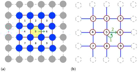
Figure 4. Building a lattice-based surrogate model for the continuous model in the equally spaced obstacles case: (a) nine subdomains are used to exploit symmetry of the obstacle arrangement. and transitions between subdomains are tracked. (b) Lattice-based surrogate representation is shown, with red circles denoting corresponding subdomains in the continuous model.

Results of the continuous model simulations (Figure 4a) are tracked via the time course $\eta \left(t_k\right)(t_k=k\Delta t,k=0,\dots ,N)$, where N is the total number of time steps. $\eta \left(t_k\right)$ records the state of a particle as the index of the ith subdomain $(i=1,\dots ,9)$ at time $t_k$ if its center is located in that subdomain at time $t_k$. A $9\times 9$ matrix $S^{\left(k\right)}$ is used to track all transitions (including remaining in the same subdomain) up to the current time step ($S^{\left(0\right)}$ is the zero matrix). $S^{\left(k\right)}$ is updated according to the formula

$$S^{\left(k\right)}\left(\eta \left(t_{k-1}\right),\eta \left(t_k\right)\right)=S^{(k-1)}\left(\eta \left(t_{k-1}\right),\eta \left(t_k\right)\right)+1,k=1,\dots N.$$

(12)

$S^{\left(k\right)}$ is then used to build a vector ${\overrightarrow{p}}^E$ of transition probabilities. Within each time step, a vector ${\overrightarrow{T}}_i^E$ ($i=1,\dots ,9$) is created to count transitions that occurred for each subdomain. In particular, the rows of $S^{\left(k\right)}$ are used to create vector ${\overrightarrow{T}}_i^E$ by grouping transition sums by transition type; since the equally spaced obstacles model has two transition types, ${\overrightarrow{T}}_i^E$ has dimensions of $1\times 2$. At the current time $t_k$, we construct ${\overrightarrow{T}}_i^E$ from $S^{\left(k\right)}$ as follows,

$${\overrightarrow{T}}_i^E=\left[S^{\left(k\right)}(i,i),\sum _{\{j\ne i\}}{S}^{\left(k\right)}(i,j)\right],i=1,\dots ,9.$$

(13)

Due to the symmetries in the equally spaced obstacles case, we create the transition probability vector ${\overrightarrow{p}}^E$ via the average:

$${\overrightarrow{p}}^E=\frac{1}{N}\sum _{i=1}^N{\overrightarrow{T}}_i^E.$$

(14)

3.3. Multisize Obstacles Model

3.3.1. Continuous Model

For the multisize obstacles model, the RVE has one set of obstacles with a fixed obstacle radius $R_{{\mathrm{obs}}_1}$ and a second set of obstacles of radius $R_{{\mathrm{obs}}_2}$ that is varied across cases. Symmetry for this model is preserved by partitioning the RVE using a $2\times 2$ grid of subdomains (Figure 3b). We view the domain as having “columns” of obstacles; obstacles in the same column have identical radii. The particle radius and first obstacle radius are fixed at values of $R_{\mathrm{part}}=1.0$ and $R_{{\mathrm{obs}}_1}=1.0$, respectively. The second obstacle radius ($R_{{\mathrm{obs}}_2}$) is then varied between $0.5$ to $3.0$ in increments of $0.5$.

3.3.2. Lattice-Based Surrogate Model

Figure 5 illustrates the construction of the 2D lattice-based surrogate model for the multisize obstacles case. A periodic extension of the RVE is shown, with primary transitions from subdomain 1 (top-left corner) illustrated. Due to inherent symmetries, all subdomains have the same number of distinct transition types. There are four types of transition with corresponding probabilities (Figure 5b). In type 1, the particle stays in its current subdomain ($p_1^M$). In types 2–4, it transitions to a neighboring subdomain (2,3 or 4) having two obstacles. We delineate the three latter types into probabilities as follows: the two obstacles are of different sizes ($R_{{\mathrm{obs}}_1}$, $R_{{\mathrm{obs}}_2}$) along the boundary ($p_2^M$); the two obstacles are the same size $R_{{\mathrm{obs}}_2}$ along the boundary ($p_3^M$); or the two obstacles are the same size $R_{{\mathrm{obs}}_1}$ along the boundary ($p_4^M$). Again, the probabilities must sum to one; the three surrogate model probabilities need to be calculated from the results of the continuous model simulations.

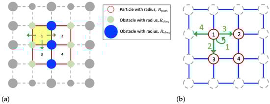
Figure 5. Building a lattice-based surrogate model for the continuous model in the multisize obstacles case: (a) four subdomains are used to exploit symmetries of the obstacle arrangement, and transitions between subdomains are tracked. Smaller green circles indicate obstacles of fixed radius $R_{{\mathrm{obs}}_1}=1.0$, and larger blue circles indicate obstacles with varying obstacle radius $R_{{\mathrm{obs}}_2}$; (b) lattice-based surrogate representation with red circles denoting corresponding subdomains in the continuous model.

Again, the time course $\eta \left(t_k\right)$ records the state of the particle as the index of the ith subdomain ($i=1,...,4$) at time $t_k$ if its center is located in that subdomain at time $t_k$. For the multisize obstacles case, we differentiate between a horizontal transition within the RVE versus a horizontal transition into an extended domain by introducing an additional time course $\zeta \left(t_k\right)(t_k=k\Delta t,k=0,\dots ,N)$, where

$$\begin{array}{c}\hfill \zeta \left(t_k\right)=\left\{\begin{array}{cc}1\hfill & \mathrm{if}\mathrm{a}\mathrm{horizontal}\mathrm{transition}\mathrm{occurred}\mathrm{into}\mathrm{an}\mathrm{extended}\mathrm{domain}\hfill \\ 0\hfill & \mathrm{otherwise}(\mathrm{includes}\mathrm{all}\mathrm{vertical}\mathrm{transitions}).\hfill \end{array}\right..\end{array}$$

(15)

In this case, the transition matrix $S^{\left(k\right)}$(for time steps $k=1,\dots ,N$) is a $4\times 5$ (augmented) matrix; the fifth column tracks horizontal transitions occurring when the particle moves into an extended domain. For a large majority of time steps, $\zeta \left(t_k\right)=0$ and $S^{\left(k\right)}$ are updated in a similar manner as in the equally spaced obstacles case via Equation (12) (Section 3.2.2). Alternatively, when $\zeta \left(t_k\right)=1$, only the new column in the augmented matrix is updated via the formula

$$S^{\left(k\right)}(\eta \left(t_{k-1}\right),5)=S^{\left(k\right)}(\eta \left(t_{k-1}\right),5)+1,k=1,...,N.$$

(16)

and $S^{\left(k\right)}$ is then used to build the vector ${\overrightarrow{p}}^M$ of five transition probabilities.

Within each time step and for each of the four subdomains, a vector ${\overrightarrow{T}}_i^M$ ($i=1,2,3,4$) is created to count transitions, according to the following rules: (i) the first component counts the number of times a particle stayed in its current subdomain; (ii) the second component counts the number of times a particle moved vertically; (iii) the third component counts the number of times a particle moved horizontally but remained in the original RVE; (iv) the fourth component counts the number of times a particle moved horizontally but moved to the extended domain.

Due to the symmetries in this case, we create the transition probability vector ${\overrightarrow{p}}^M$ via the average:

$${\overrightarrow{p}}^M=\frac{1}{N}\sum _{j=1}^N{\overrightarrow{T}}_j^M.$$

(17)

4. Model Calibration and Square Lattice Surrogate Models

4.1. Commitment Index

For random walks in our continuous model, a particle may cross, return and then recross a subdomain boundary several times before “committing” to a new subdomain. This leads to inaccuracy in the calculation of transition probabilities as stationary quantities in the lattice-based surrogate models. Consequently, we introduce a commitment index, $M_C$, to indicate the number of successive time steps after which a particle is deemed to commit to a new subdomain. The role of this parameter is illustrated in Figure 6 for the case $M_C=4$. While the value of $M_C$ requires calibration via direct comparison of simulated results for mean-squared displacement in the continuous and lattice-based surrogate models, we now explain its narrow range of variation.

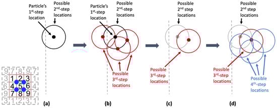
Figure 6. Illustration of the role of the commitment index (calibration) parameter $M_C$: (a) The particle (solid black circle) has just crossed the boundary between subdomains (dashed gray line) to reach its 1st-step location. Possible 2nd-step locations are indicated by the solid black ring. (b) Three possible 2nd-step locations are indicated by solid red circles. Some possible next steps (3rd-step locations) are shown with red rings. (c) A red ring illustrates the particle’s remaining possible 3rd-step locations when it has remained in the current subdomain at the prior step. (d) Possible 4th-step locations are indicated with blue rings.

(i)

Consider a particle, committed to a subdomain, that has just crossed the boundary into a neighboring subdomain (first-step location). A (black) ring indicates all possible particle locations at the next step, including some locations that result in recrossing the same boundary (Figure 6a).

(ii)

We next illustrate a few possible steps relative to the particle’s first-step location, thus indicating possible second-step locations. A (red) ring of possible 3rd-step locations is shown around each such second-step location (Figure 6b).

(iii)

Choosing one of the possible second-step locations that is in the new subdomain (gray ring), the resulting set of possible third-step locations is shown in red (Figure 6c).

(iv)

Lastly, the larger the number of successive steps for which a particle remains in the new subdomain, the smaller the probability that it will recross back into the subdomain to which it was previously committed; in Figure 6d, blue rings depict fourth-step locations.

For each of our two obstacle arrangements, $M_C$ is calibrated by constructing transition probabilities from continuous model simulations over a range of $M_C$ values and by comparing mean-squared displacement for the continuous and lattice-based surrogate models to identify the case with the best agreement (see Section 5.1).

4.2. Diffusivities for the Square Lattice Surrogate Models

Recall from Section 2 the following estimates of the effective diffusivity (e.g., (2) with $d=2$) for the continuous model and the surrogate model, respectively,

$${\kappa }_{\mathrm{cont}}=\frac{⟨r_{\mathrm{cont}}^2⟩}{4N\Delta t},\mathrm{and}{\kappa }_{\mathrm{surr}}=\frac{⟨r_{\mathrm{surr}}^2⟩}{4N\Delta t}.$$

(18)

In Section 4.2, we use 2D Taylor series expansions to derive the (continuum) diffusion equation and the associated theoretical diffusivities on a lattice for both obstacle arrangements.

4.2.1. Equally Spaced Obstacles Model

Consider a 2D rectangular lattice with horizontal spacing $h(=\Delta x)$ and vertical spacing $k(=\Delta y)$. Assuming a fixed volume and a uniform particle mass, let $u(x,y,t)$ be the density of particles and let q be the probability that a particle stays in its current subdomain; $(1-q)$ is the probability of transitioning to a neighboring lattice point. The resulting particle density is given by

$$\begin{array}{cc}\hfill u(x,y,t+\Delta t)& =qu(x,y,t)\hfill \\ \hfill & +\frac{1}{4}(1-q)\left[u(x+h,y,t)+u(x-h,y,t)+u(x,y+k,t)+u(x,y-k,t)\right].\hfill & \hfill \hspace{1em}\end{array}$$

(19)

Consider the Taylor series expansions about the point $P(x,y,t)$,

$$\begin{array}{c}\hfill u(x,y,t+\Delta t)=u+u_t(\Delta t)+\frac{1}{2}{u}_{tt}{(\Delta t)}^2+\frac{1}{6}{u}_{ttt}{(\Delta t)}^3+...,\end{array}$$

(20)

$$u(x\pm h,y,t)=u\pm u_x(\Delta x)+\frac{1}{2}{u}_{xx}{(\Delta x)}^2\pm \frac{1}{6}{u}_{xxx}{(\Delta x)}^3+...,$$

(21)

$$u(x,y\pm k,t)=u\pm u_y(\Delta y)+\frac{1}{2}{u}_{yy}{(\Delta y)}^2\pm \frac{1}{6}{u}_{yyy}{(\Delta y)}^3+....$$

(22)

Using these series expansions, (19) becomes

$$u_t(\Delta t)+\mathcal{O}\left({(\Delta t)}^2\right)=\frac{(1-q)}{4}\left[u_{xx}{(\Delta x)}^2+u_{yy}{(\Delta y)}^2+\mathcal{O}\left({(\Delta y)}^4\right)+\mathcal{O}\left({(\Delta x)}^4\right)\right].$$

(23)

Assuming a 2D square lattice ($\Delta x=\Delta y$) and dividing by $\Delta t$, we can rewrite (23) as

$$u_t+\mathcal{O}(\Delta t)=\frac{(1-q)}{4}\left(u_{xx}\frac{{(\Delta x)}^2}{(\Delta t)}+u_{yy}\frac{{(\Delta x)}^2}{(\Delta t)}+\mathcal{O}\left(\frac{{(\Delta x)}^4}{(\Delta t)}\right)\right),$$

(24)

resulting in the approximate equation (assuming $(1-q){(\Delta x)}^4\ll \Delta t$),

$$u_t\approx \frac{(1-q){(\Delta x)}^2}{4(\Delta t)}\left(u_{xx}+u_{yy}\right).$$

(25)

Recognizing (25) as the 2D diffusion equation, the theoretical diffusivity for the equal obstacles model (D) is given in terms of square lattice model properties by

$$D=\frac{(1-q){(\Delta x)}^2}{4(\Delta t)}.$$

(26)

4.2.2. Multisize Obstacles Model

In the multisize obstacles model, the particle has different diffusivities in the vertical and horizontal directions. Yet, the large majority of lattice-based models in computational biology employ a square lattice. Thus, while our derivation below allows for distinct values of $\Delta x$ and $\Delta y$, we ultimately set these quantities to be equal in order to reconcile the two viewpoints.

We follow the same procedure as in Section 4.2.1, but for this case, note the following: (i) $q_1$ is the probability that the particle stays at its current lattice point; (ii) $q_x$ is the probability that the particle moves to a neighboring lattice point in the horizontal direction; (iii) $q_y$ is the probability that the particle moves to a neighboring lattice point in the vertical direction. Note that $q_1+q_x+q_y=1$. We can then write the following relation for the particle density:

$$\begin{array}{cc}\hfill u(x,y,t+\Delta t)=& q_{1}u(x,y,t)+\frac{q_x}{2}u(x+h,y,t)+\frac{q_x}{2}u(x-h,y,t)\hfill \\ \hfill & +\frac{q_y}{2}u(x,y+k,t)+\frac{q_y}{2}u(x,y-k,t).\hfill \end{array}$$

(27)

Via the Taylor series expansions in (20)–(22), the above equation can be expanded and simplified to

$$\begin{array}{cc}\hfill u+u_t(\Delta t)& +\mathcal{O}\left({(\Delta t)}^2\right)=q_{1}u+q_{x}u+q_{y}u+\frac{q_x}{2}\left(u_{xx}{(\Delta x)}^2+\mathcal{O}\left({(\Delta x)}^4\right)\right)\hfill \\ \hfill & +\frac{q_y}{2}\left(u_{yy}{(\Delta y)}^2+\mathcal{O}\left({(\Delta y)}^4\right)\right).\hfill \end{array}$$

(28)

Since $q_1+q_x+q_y=1$, upon dividing by $\Delta t$ we can rewrite (28) as

$$u_t+\mathcal{O}(\Delta t)=\frac{q_x}{2}{u}_{xx}\frac{{(\Delta x)}^2}{(\Delta t)}+\frac{q_y}{2}{u}_{yy}\frac{{(\Delta y)}^2}{(\Delta t)}+\frac{q_x}{2}\mathcal{O}\left(\frac{{(\Delta x)}^4}{(\Delta t)}\right)+\frac{q_y}{2}\mathcal{O}\left(\frac{{(\Delta y)}^4}{(\Delta t)}\right).$$

(29)

Imposing our restriction to a uniform 2D lattice ($\Delta x=\Delta y$), the simplified diffusion equation for the multisize obstacles case is thus (assuming $q_x{(\Delta x)}^4\ll \Delta t$ and $q_y{(\Delta x)}^4\ll \Delta t$)

$$u_t\approx \frac{{(\Delta x)}^2}{2(\Delta t)}\left(q_x{u}_{xx}+q_y{u}_{yy}\right).$$

(30)

Hence, when a 2D square lattice is used as a surrogate model for the multisize obstacles case, there are two theoretical diffusivities that we refer to as the horizontal diffusivity ($D_H$) and the vertical diffusivity ($D_V)$, which are given by

$$D_H=\frac{q_x{(\Delta x)}^2}{2(\Delta t)},D_V=\frac{q_y{(\Delta x)}^2}{2(\Delta t)}.$$

(31)

We note that in the case $q_x=q_y$, the diffusion equation for the multisize obstacles model (30) reduces to the diffusion equation for the equally spaced obstacles model (25).

4.3. Relating the Diffusivities

We now relate our effective diffusivities (${\kappa }_{\mathrm{cont}},{\kappa }_{\mathrm{surr}})$ in (18) to the theoretical diffusivities for each of the two obstacle models, i.e., (26) and (31).

4.3.1. Equally Spaced Obstacles Model

The effective diffusivity for the surrogate model ${\kappa }_{\mathrm{surr}}$ is first used to approximate the effective diffusivity for the continuous model ${\kappa }_{\mathrm{cont}}$. Specifically, slopes of the mean squared displacement response are matched by calibrating the commitment index $M_C$ in the surrogate model (see Section 4.1).

Substituting $⟨r^2⟩$ from (11) for the surrogate model into the second relation of (18), we obtain the relations,

$$\begin{array}{cc}\hfill {\kappa }_{\mathrm{surr}}& =\frac{⟨r_{\mathrm{surr}}^2⟩}{4N\Delta t}\approx \frac{N(1-q){(\Delta x)}^2}{4N\Delta t}=\frac{(1-q){(\Delta x)}^2}{4\Delta t}=D.\hfill \end{array}$$

(32)

Since $\Delta t$ is the same across all representations, it remains to calibrate $\Delta x$, i.e., the effective spatial grid size for the square lattice model with theoretical diffusivity D.

Although $L=10$ is a characteristic length scale for both the continuous and (surrogate) lattice models, it is not an appropriate choice for $\Delta x$ in (32). A particle at an arbitrary location in a subdomain has many different net distances it can travel before crossing into and committing to a neighboring subdomain. We determine the spatial step size via the representation $\Delta x=\frac{L}{\alpha }$, where $\alpha >1$ will be calibrated based on our numerical simulations.

Substituting $\Delta x=\frac{L}{\alpha }$ into (32), we obtain

$$\begin{array}{cc}\hfill {\kappa }_{\mathrm{surr}}& \approx D{|}_{\Delta x=\frac{L}{\alpha }}=\frac{(1-q){\left(\frac{L}{\alpha }\right)}^2}{4\Delta t}=\frac{1}{{\alpha }^2}D{|}_{\Delta x=L}.\hfill \end{array}$$

(33)

Hence, the ratio of the two diffusivities can be used to approximate $\alpha$ via the formula

$$\alpha \approx \sqrt{\frac{D{|}_{\Delta x=L}}{{\kappa }_{\mathrm{surr}}}}.$$

(34)

Using this coordinated approach, we ensure that all diffusivity estimates obtained via simulations using the continuous model and the surrogate model are consistent with theoretical estimates for 2D random walks on a lattice based on the choice $\Delta x=\frac{L}{\alpha }$.

4.3.2. Multisize Obstacles Model

Considering the horizontal and vertical effective diffusivities independently, and using (2) with $d=1$, we can define ${\kappa }_H$ and ${\kappa }_V$ as

$${\kappa }_H=\frac{⟨r_H^2⟩}{2N\Delta t},{\kappa }_V=\frac{⟨r_V^2⟩}{2N\Delta t},$$

(35)

where $⟨r_H^2⟩$ and $⟨r_V^2⟩$ are the horizontal and vertical mean squared displacements. In the multisize obstacles model, we identified horizontal and vertical components of diffusivity in terms of the corresponding probabilities (see (31)).

In contrast to the equally spaced obstacles model, here we do not directly identify the probabilities $q_x$ (of a horizontal transition) and $q_y$ (of a vertical transition) in the square lattice surrogate model. In particular, $q_x$ is not explicitly identified from our simulations, since our results delineate (1) a horizontal transition in the original RVE and (2) a horizontal transition to the extended domain. We, instead, relate the following ratios:

$$\frac{D_H}{D_V}\approx \frac{{\kappa }_H}{{\kappa }_V}\approx \frac{⟨r_H^2⟩}{⟨r_V^2⟩}\approx \frac{q_x}{q_y}.$$

(36)

Note that in the case where all obstacles are the same size, this yields $D_H\approx D_V$.

For the lattice-based surrogate model, the four probabilities $p_1,p_2,p_3,p_4$ correspond to the transitions depicted in Figure 5b. Recall that $q_1+q_x+q_y=1$ in the square lattice surrogate model and $p_1+2p_2+p_3+p_4=1$ in the lattice-based surrogate model. Equating these two relations and assuming that $q_1=p_1$ and that $2p_2=q_y$, we obtain the reduced equation

$$q_x=p_3+p_4.$$

(37)

Assuming ${\kappa }_H\approx D_H$ and ${\kappa }_V\approx D_V$, we can use simulation results to calibrate $\Delta x$ using each of the two relations in (31) (see Section 5.2.2). Moreover, we note that the ratio of diffusivities in (36) is independent of the square lattice grid size.

5. Results

For both the equally spaced obstacles model (Section 3.2) and the multisize obstacles model (Section 3.3), we use results of the continuous model simulations to determine transition probabilities for the two surrogate models, as described in Section 3.2.2 and Section 3.3.2, respectively. As outlined in Section 3.1, we simulate a single particle (radius $R_{\mathrm{part}}$) undergoing a 2D random walk (speed $v=8$) with time step $\Delta t=0.05$. At each step, the direction is sampled from a uniform distribution and all collisions with internal obstacles are perfectly elastic. All continuous model simulations were carried out on a high-performance cluster computer for $N=2000$ realizations. Once transition probabilities were determined, the corresponding lattice-based surrogate model simulations were carried out on a laptop computer (MacBook Pro) in under 2.5 h. By contrast, the continuous model simulations were completed at a rate of 400 realizations per 27 h, distributed over eight processors (50 realizations per processor), for a specified set of model parameters. A total of $N_t=1\times {10}^7$ time steps were sufficient for all quantities of interest to exhibit stationary responses.

5.1. Building the Lattice-Based Surrogate Models

5.1.1. Equally Spaced Obstacles Case

Obstacle radii: Continuous model simulations were performed on the RVE for the equally spaced obstacles model (see Section 3.2.1 and Figure 3a). The particle radius was first fixed at $R_{\mathrm{part}}=1.0$, and the obstacle radius ($R_{\mathrm{obs}}$) was varied from $0.5$ to $3.0$ by increments of 0.5. Stationarity and linearity of $⟨r^2⟩$ versus time (Section 2.1) for an increasing number of realizations is illustrated, for a representative case ($R_{\mathrm{part}}=1.0$, $R_{\mathrm{obs}}=1.0$), in Figure 7.

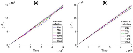
Figure 7. Mean squared displacement versus time for the equally spaced obstacles model. Effects of an increasing number of realizations are shown for the case $R_{\mathrm{part}}=1.0$ and $R_{\mathrm{obs}}=1.0$: (a) curves; (b) linear fits to the curves.

Determining transition probabilities: Based on the approach illustrated in Figure 4, continuous model results were used to determine transition probabilities for the equally spaced obstacles model via (14). These probabilities are illustrated for transitions from subdomain 6 over the time course of one realization in Figure 8b–d; rescaling the range more effectively illustrates the stay and leave probabilities (Figure 8c,d, respectively). This figure also demonstrates the stationary nature of these probabilities at later times. In determining the final stay ($p^E\left(1\right)$) and leave ($p^E\left(2\right)$) transition probabilities for the lattice-based surrogate model, values of each type were pooled together (see (14)) and then averaged across all realizations. Note that our results are consistent with the improbability of diagonal transitions (Figure 8d, blue curve).

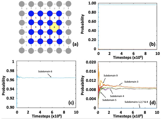
Figure 8. Transition probabilities for building the lattice-based surrogate model from the equally spaced obstacles (continuous) model. Transitions from subdomain 6 are illustrated: (a) simulation domain showing the 9 subdomains; (b) plot of all transition probabilities (here, only the stay probability is discernible); (c) magnified plot to illustrate the stay probability; (d) magnified plot to illustrate the leave probabilities.

Commitment index calibration: Lattice-based surrogate models were built using the transition probabilities obtained from the continuous model (see (14), Section 3.2.2) by first calibrating the commitment index $M_C$ (Section 4.1). $M_C$ was varied from 3 to 8 and calibrated by comparing the continuous and surrogate plots of $⟨r^2⟩$ versus time. This procedure was repeated for varying obstacle radii, with the particle radius fixed at $R_{\mathrm{part}}=1.0$, illustrated in Figure 9 for $R_{\mathrm{part}}=1.0$ and $R_{\mathrm{obs}}=2.0$. Here, $M_C=5$ yields the best result; 2000 realizations were sufficient to observe stationary values sufficient to calibrate $M_C$ (Figure 9—right). Probabilities and commitment index values are shown in Table 1. We observe that the sum of the first probability and four times the second probability is very close to 1 (based on symmetries in the RVE); the largest discrepancy was observed to be $3.6\times {10}^{-6}$. We also observe that the probability of staying in the current subdomain increases with the obstacle radius. Comparisons of slopes for $⟨r^2⟩$ versus time for the continuous and surrogate models are compared in Table 2 and Figure 10. We observe differences in slopes ranging from 0.004% to roughly 4%.

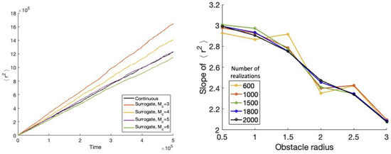
Figure 9. Mean squared displacement and its slope for the equally spaced obstacles model. Results are shown for particle radius $R_{\mathrm{part}}=1.0$ and obstacle radius $R_{\mathrm{obs}}=2.0$: (left) $⟨r^2⟩$ versus time for continuous model and resulting surrogate model as the commitment index $M_c$ is varied; (right) slope as a function of obstacle radius for an increasing number of realizations.

Table 1. Transition probabilities in the lattice-based surrogate model for the equally spaced obstacles (continuous) model for the best values of $M_c$ with particle radius $R_{\mathrm{part}}=1.0$.

		Probability by Transition Type
${\mathit{R}}_{\mathbf{obs}}$	${\mathit{M}}_{\mathit{c}}$	${\mathit{p}}_{\mathbf{1}}^{\mathit{E}}$	${\mathit{p}}_{\mathbf{2}}^{\mathit{E}}$
0.5	7	$0.99276$	$1.8099\times {10}^{-3}$
1.0	6	$0.99291$	$1.7724\times {10}^{-3}$
1.5	5	$0.99297$	$1.7573\times {10}^{-3}$
2.0	5	$0.99371$	$1.5734\times {10}^{-3}$
2.5	4	$0.99384$	$1.5401\times {10}^{-3}$
3.0	4	$0.99493$	$1.2676\times {10}^{-3}$

Table 2. Slope values for $⟨r^2⟩$ vs. t in the equally spaced obstacles (continuous) model ($R_{\mathrm{part}}=1.0$) and the lattice-based surrogate model. The best values of $M_C$ are also shown.

${\mathit{R}}_{\mathbf{obs}}$	${\mathit{M}}_{\mathit{c}}$	Slope (Continuous)	Slope (Surrogate)	Percent Difference
0.5	7	2.9984	2.8770	4.049%
1.0	6	2.9044	2.8468	1.983%
1.5	5	2.7507	2.7506	0.004%
2.0	5	2.4731	2.5094	1.468%
2.5	4	2.3376	2.4310	3.996%
3.0	4	2.0765	2.1016	1.209%

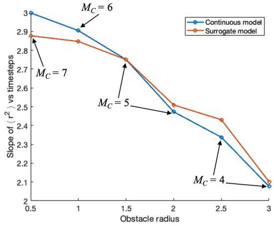
Figure 10. Slope of $⟨r^2⟩$ versus time for equally spaced obstacles (continuous) model and the lattice-based surrogate model with best $M_c$ values. Results are shown for particle radius $R_{\mathrm{part}}=1.0$ and varying obstacle radius $R_{\mathrm{obs}}$.

5.1.2. Multisize Obstacles Case

Obstacle radii: Continuous model simulations were also performed for the multisize obstacles model (Figure 5) on an RVE partitioned into four subdomains as described in Section 3.3.1. The particle radius was fixed at $R_{\mathrm{part}}=1.0$, with one obstacle radius fixed at $R_{{\mathrm{obs}}_1}=1.0$ and the other obstacle radius ($R_{{\mathrm{obs}}_2}$) varied from $0.5$ to $3.0$ in increments of 0.5. Stationarity and linearity of $⟨r^2⟩$ versus time is illustrated, for a representative case ($R_{\mathrm{part}}=1.0$, $R_{{\mathrm{obs}}_1}=1.0$ and $R_{{\mathrm{obs}}_2}=1.0$), in Figure 11.

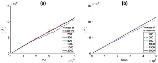
Figure 11. Mean squared displacement versus time for the multisize obstacles model. Effects of an increasing number of realizations are shown for the case $R_{\mathrm{part}}=1.0$, $R_{{\mathrm{obs}}_1}=1.0$ and $R_{{\mathrm{obs}}_2}=1.5$: (a) curves; (b) linear fits to the curves.

Determining transition probabilities: Based on the approach illustrated in Figure 5, continuous model results were used to determine transition probabilities for the multisize obstacles model using (17).

Commitment index calibration: Lattice-based surrogate models were built using the transition probabilities obtained from the continuous model (Section 3.3.2) by first calibrating the commitment index $M_C$ (Section 4.1). For each case considered, $M_C$ was varied from 3 to 8 and calibrated by comparing the continuous and surrogate plots of $⟨r^2⟩$ versus time. A sample plot illustrates increasing stationarity of the slope of $⟨r^2⟩$ versus obstacle radius as the number of realizations increases (Figure 12—left).

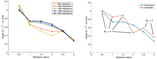
Figure 12. Slope of the mean squared displacement for the multisize obstacles model: (left) variation with obstacle radius as the number of realizations is increased; (right) comparison of the continuous and lattice-based surrogate models for the best $M_C$ values.

We observe the manner in which the slope decreases with increasing obstacle radius $R_{{\mathrm{obs}}_2}$, which differs from that observed in the equally spaced obstacles case (Figure 10). A summary of the transition probabilities and values of $M_C$ needed to build the lattice-based surrogate model for all cases considered is provided in Table 3. Note that the sum of the probabilities in each row is 1 when the second probability is weighted by a factor of 2 due to symmetries in the RVE.

Table 3. Transition probabilities in the lattice-based surrogate model for the multisize obstacles (continuous) model for the best values of $M_c$ with particle radius $R_{\mathrm{part}}=1.0$ and $R_{{\mathrm{obs}}_1}=1.0$.

		Probability by Transition Type
${\mathit{R}}_{{\mathbf{obs}}_{\mathbf{2}}}$	${\mathit{M}}_{\mathit{c}}$	${\mathit{p}}_{\mathbf{1}}^{\mathit{M}}$	${\mathit{p}}_{\mathbf{2}}^{\mathit{M}}$	${\mathit{p}}_{\mathbf{3}}^{\mathit{M}}$	${\mathit{p}}_{\mathbf{4}}^{\mathit{M}}$
0.5	6	$0.99253$	$1.8680\times {10}^{-3}$	$2.0159\times {10}^{-3}$	$1.7147\times {10}^{-3}$
1.0	6	$0.99291$	$1.7715\times {10}^{-3}$	$1.7764\times {10}^{-3}$	$1.7725\times {10}^{-3}$
1.5	6	$0.99324$	$1.6894\times {10}^{-3}$	$1.5339\times {10}^{-3}$	$1.8510\times {10}^{-3}$
2.0	6	$0.99352$	$1.6203\times {10}^{-3}$	$1.2909\times {10}^{-3}$	$1.9522\times {10}^{-3}$
2.5	5	$0.99316$	$1.7098\times {10}^{-3}$	$1.1322\times {10}^{-3}$	$2.2850\times {10}^{-3}$
3.0	5	$0.99339$	$1.6502\times {10}^{-3}$	$8.1439\times {10}^{-4}$	$2.4950\times {10}^{-3}$

Comparisons of slopes for the relation between $⟨r^2⟩$, including the best values for $M_C$, are shown for the continuous and surrogate models in Table 4 and Figure 12—right. These results exhibit a difference in slopes ranging from 0.6% to roughly 7%.

Table 4. Slope values for $⟨r^2⟩$ vs. t in the multisize obstacles (continuous) model ($R_{\mathrm{part}}=1.0$, $R_{{\mathrm{obs}}_1}=1.0$) and the lattice-based surrogate model. The best values of $M_C$ are also shown.

${\mathit{R}}_{{\mathbf{obs}}_2}$	${\mathit{M}}_{\mathit{c}}$	Slope (Continuous)	Slope (Surrogate)	Percent Difference
0.5	6	2.9870	3.0059	0.632%
1.0	6	2.7357	2.8531	4.291%
1.5	6	2.7376	2.8939	5.709%
2.0	6	2.6618	2.4751	7.014%
2.5	5	2.4995	2.5904	3.637%
3.0	5	2.2710	2.3651	4.144%

5.2. Estimating Diffusivities

We use the continuous and lattice-based surrogate model results to estimate effective and theoretical diffusivities (see Figure 1).

5.2.1. Equally Spaced Obstacles Case

We estimate the effective diffusivities from simulated results for the mean squared displacement in both the continuous (${\kappa }_{\mathrm{cont}}$) and surrogate (${\kappa }_{\mathrm{surr}}$) models via (18) and for each obstacle radius (Figure 13).

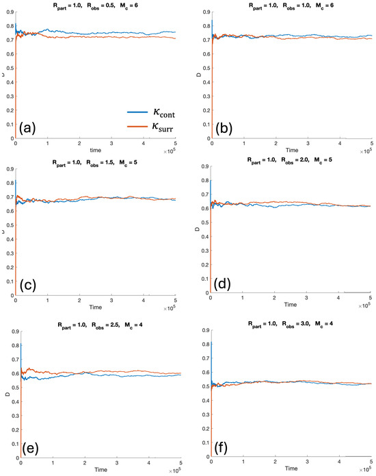
Figure 13. Estimated effective diffusivities for the continuous and lattice-based surrogate models in the equally spaced obstacles case with $R_{\mathrm{part}}=1.0$: (a) $R_{\mathrm{obs}}=0.5$, $M_C=6$; (b) $R_{\mathrm{obs}}=1.0$, $M_C=6$; (c) $R_{\mathrm{obs}}=1.5$, $M_C=5$; (d) $R_{\mathrm{obs}}=2.0$, $M_C=5$; (e) $R_{\mathrm{obs}}=2.5$, $M_C=4$; (f) $R_{\mathrm{obs}}=3.0$, $M_C=4$.

Time averages for both effective diffusivities over the last 100,000 values are shown in Table 5, along with the commitment index $M_C$ and the stay probability q. The continuous and surrogate diffusivities exhibit a correlation coefficient of $R=0.9784$ and percent differences between $0.02\%$ and roughly $6\%$.

Table 5. Effective diffusivities in the equally spaced obstacles case for the continuous model (${\kappa }_{\mathrm{cont}}$) and the lattice-based surrogate model (${\kappa }_{\mathrm{surr}}$). The stay probability (q) and best commitment index ($M_C$) are also shown for each obstacle radius ($R_{\mathrm{obs}}$).

${\mathit{R}}_{\mathbf{obs}}$	${\mathit{M}}_{\mathit{C}}$	q	${\mathit{\kappa }}_{\mathbf{cont}}$	${\mathit{\kappa }}_{\mathbf{surr}}$	Percent Difference
0.5	7	0.99276	0.7550	0.7100	5.960%
1.0	6	0.99291	0.7314	0.7084	3.145%
1.5	5	0.99297	0.6759	0.6862	1.524%
2.0	5	0.99371	0.6146	0.6165	0.309%
2.5	4	0.99384	0.5885	0.6016	2.226%
3.0	4	0.99493	0.5188	0.5187	0.019%

Estimated diffusivities for the surrogate models were used to compute values of ${\alpha }^2$ and $\Delta x(=\frac{L}{\alpha })$, for each case. Comparisons of the effective diffusivities to the resulting theoretical diffusivities, determined via (33), are shown in Table 6. For comparison, the theoretical estimate of the diffusivity for the case $L=10$, corresponding to ${\alpha }^2=1$, is also shown in the table. The estimated values of both ${\alpha }^2$ (mean 5.0466, st. dev. 0.0888) and $\Delta x$ (mean 4.4519, st. dev. 0.0397) exhibited little variation or correlation ($R=0.5532$) across the range of obstacle sizes considered. This finding suggests that the coefficient ${\alpha }^2$ can be approximated as constant across the range of obstacle radii considered.

Table 6. Theoretical diffusivity (D) and grid size ($\Delta x$) in the equally spaced obstacles case. The stay probability (q), best commitment index ($M_C$) and theoretical diffusivity with $L=10$ (${D|}_{\Delta x=10}$) are also shown for each obstacle radius ($R_{\mathrm{obs}}$).

${\mathit{R}}_{\mathbf{obs}}$	q	${\mathit{\alpha }}^2$	$\mathbf{\Delta }\mathit{x}$	${\mathit{\kappa }}_{\mathbf{cont}}$	${\mathit{\kappa }}_{\mathbf{surr}}$	D	${\mathit{D}|}_{\mathit{\Delta }\mathit{x}=10}$
0.5	0.99276	5.1048	4.4260	0.7550	0.7100	0.7100	3.6243
1.0	0.99291	5.0027	4.4709	0.7314	0.7084	0.7084	3.5440
1.5	0.99297	5.1224	4.4184	0.6759	0.6862	0.6862	3.5149
2.0	0.99371	5.0907	4.4321	0.6146	0.6165	0.6165	3.1384
2.5	0.99384	5.0728	4.4399	0.5885	0.6016	0.6016	3.0517
3.0	0.99493	4.8863	4.5239	0.5188	0.5187	0.5187	2.5343

The 2D lattice-based surrogate model for the equally spaced obstacles case is thus fully represented by the set of parameters $q,p(=1-q),\Delta x$ and $\alpha$ shown in Table 6 for each obstacle radius.

5.2.2. Multisize Obstacles Case

We also estimated effective diffusivities from simulated results for the continuous and surrogate models via (18) and for each obstacle radius combination (Figure 14). Time averages for each of these effective diffusivities over the last 100,000 values are shown in Table 7 along with the commitment index $M_C$ and the stay probability q. The continuous and surrogate diffusivities exhibit a correlation coefficient of $R=0.8503$ and differences ranging between roughly $1.1\%$ and $6.8\%$.

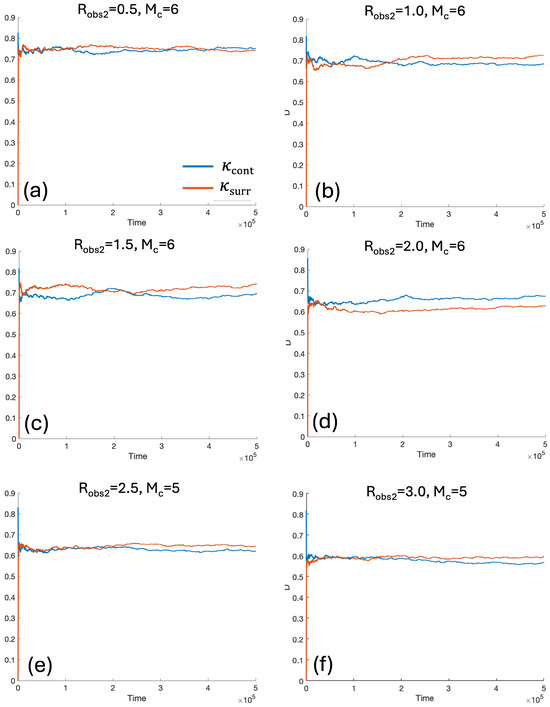
Figure 14. Estimated effective diffusivities for the continuous and lattice-based surrogate models in the multisize obstacles case with $R_{\mathrm{part}}=1.0$, $R_{{\mathrm{obs}}_1}=1.0$: (a) $R_{{\mathrm{obs}}_2}=0.5$, $M_c=6$; (b) $R_{{\mathrm{obs}}_2}=1.0$, $M_c=6$; (c) $R_{{\mathrm{obs}}_2}=1.5$, $M_c=6$; (d) $R_{{\mathrm{obs}}_2}=2.0$, $M_c=6$; (e) $R_{{\mathrm{obs}}_2}=2.5$, $M_c=6$; (f) $R_{{\mathrm{obs}}_2}=3.0$, $M_c=6$.

Table 7. Effective diffusivities in the multisize obstacles case for the continuous model (${\kappa }_{\mathrm{cont}}$) and the lattice-based surrogate model (${\kappa }_{\mathrm{surr}}$). The resulting stay probability ($q_1$) in the square lattice surrogate model and the best commitment index ($M_C$) are also shown for each obstacle radius ($R_{\mathrm{obs}}$).

${\mathit{R}}_{\mathbf{obs}}$	${\mathit{M}}_{\mathit{c}}$	${\mathit{q}}_1$	${\mathit{\kappa }}_{\mathbf{cont}}$	${\mathit{\kappa }}_{\mathbf{surr}}$	Percent Difference
0.5	6	0.9925	0.7509	0.7428	1.084%
1.0	6	0.9929	0.6842	0.7261	6.133%
1.5	6	0.9932	0.6943	0.7418	6.845%
2.0	6	0.9935	0.6746	0.6290	6.755%
2.5	5	0.9932	0.6205	0.6440	3.785%
3.0	5	0.9939	0.5667	0.5942	4.859%

Recalling Equation (31) (Section 4.2.2), for the theoretical diffusivities in the multisize obstacles case, we write

$$D_H=\frac{q_x{(\Delta x_M)}^2}{2(\Delta t)},D_V=\frac{q_y{(\Delta x_M)}^2}{2(\Delta t)}.$$

(38)

Here, $\Delta x_M$ denotes the effective grid size for the multisize obstacles case, and its value remains to be calibrated. Note, however, that the ratio of these two diffusivities is independent of this parameter. Consequently, we first examined this ratio using (36) by evaluating the relevant mean squared displacements (Figure 15) and their ratio (Figure 16).

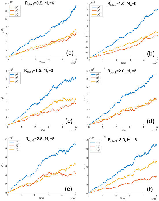
Figure 15. Horizontal, vertical and (regular) mean squared displacements for the lattice-based surrogate model in the multisize obstacles case with $R_{\mathrm{part}}=1.0$, $R_{{\mathrm{obs}}_1}=1.0$: (a) $R_{{\mathrm{obs}}_2}=0.5$, $M_c=6$; (b) $R_{{\mathrm{obs}}_2}=1.0$, $M_c=6$; (c) $R_{{\mathrm{obs}}_2}=1.5$, $M_c=6$; (d) $R_{{\mathrm{obs}}_2}=2.0$, $M_c=6$; (e) $R_{{\mathrm{obs}}_2}=2.5$, $M_c=6$; (f) $R_{{\mathrm{obs}}_2}=3.0$, $M_c=6$.

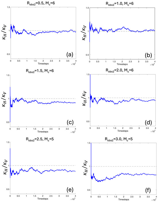
Figure 16. Ratio of horizontal and vertical diffusivities for the lattice-based surrogate model in the multisize obstacles case with $R_{\mathrm{part}}=1.0$, $R_{{\mathrm{obs}}_1}=1.0$: (a) $R_{{\mathrm{obs}}_2}=0.5$, $M_C=6$; (b) $R_{{\mathrm{obs}}_2}=1.0$, $M_C=6$; (c) $R_{{\mathrm{obs}}_2}=1.5$, $M_C=6$; (d) $R_{{\mathrm{obs}}_2}=2.0$, $M_C=6$; (e) $R_{{\mathrm{obs}}_2}=2.5$, $M_C=6$; (f) $R_{{\mathrm{obs}}_2}=3.0$, $M_C=6$.

The multisize obstacles model has the property that the RVE is more open in either the horizontal ($R_{{\mathrm{obs}}_2}<1$) or vertical ($R_{{\mathrm{obs}}_2}>1$) direction, depending on the value of $R_{{\mathrm{obs}}_2}$. This effect is subtle for $R_{{\mathrm{obs}}_2}<1$ due to the large amount of available space for particle diffusion (Figure 15a and Figure 16a). Significant effects on the ratio of diffusivities are observed for larger values in the regime $R_{{\mathrm{obs}}_2}>1$, where available space in the horizontal direction becomes more limited (Figure 15e,f and Figure 16e,f). An increased time to achieve a stationary response is also observed for these cases.

The effective grid size $\Delta x_M$ can be computed in one of two ways, by approximating $D_H$ and $D_V$ by ${\kappa }_H$ and ${\kappa }_V$, respectively, and solving the corresponding relation in (38) for $\Delta x_M$ (Table 8). The values of $\Delta x_M$ computed in this manner are $4.2268\pm 0.1444$ (mean ± SD) using ${\kappa }_H$ and $4.0684\pm 0.2099$ using ${\kappa }_V$. A single-factor ANOVA analysis results in p-values of 0.159 for $R_{ob{s}_2}$ between 0.5 and 3.0, 0.226 for $R_{ob{s}_2}$ between 0.5 and 2.5 and 0.394 for $R_{ob{s}_2}$ between 0.5 and 2.0. These findings suggest that $\Delta x_M$ can be approximated as constant, with some caution needed for the case with the largest obstacle sizes.

Table 8. Estimated values of grid size $\Delta x_M$ based on the lattice-based surrogate model simulation results for the multisize case using the effective horizontal diffusivity (${\kappa }_H$) and the effective vertical diffusivity (${\kappa }_V$). The resulting transition (leave) probabilities in the square lattice surrogate model are also shown.

${\mathit{R}}_{{\mathit{o}\mathit{b}\mathit{s}}_2}$	${\mathit{q}}_{\mathit{y}}=2{\mathit{p}}_2$	${\mathit{q}}_{\mathit{x}}={\mathit{p}}_3+{\mathit{p}}_4$	$\mathit{\Delta }{\mathit{x}}_{\mathit{M}}$ (${\mathit{\kappa }}_{\mathit{V}}$ est.)	$\mathit{\Delta }{\mathit{x}}_{\mathit{M}}$ (${\mathit{\kappa }}_{\mathit{H}}$ est.)
$0.5$	$0.0037360$	$0.0037629$	$4.2097$	$4.1652$
$1.0$	$0.0035430$	$0.0035489$	$4.0917$	$4.1101$
$1.5$	$0.0033788$	$0.0033849$	$4.3173$	$4.1280$
$2.0$	$0.0032406$	$0.0032431$	$4.4659$	$4.3340$
$2.5$	$0.0034196$	$0.0034172$	$4.1858$	$3.9538$
$3.0$	$0.0033004$	$0.0033094$	$4.0902$	$3.7193$

The 2D lattice-based surrogate model for the multisize obstacles case is thus fully represented by the set of parameters $q_x$, $q_y$, $q_1(=1-q_x-q_y)$ and $\Delta x_M$, shown for each obstacle radius in Table 8. In reality, using an average of the two calculated values of $\Delta x_M$ is recommended.

6. Discussion and Conclusions

In this study, we developed a systematic approach (outlined in Figure 1) for bridging two-dimensional continuous models of diffusive transport in the presence of rigid internal obstacles with perfectly elastic collisions with two types of surrogate models. The first type is a lattice-based surrogate model that exploits symmetries in the RVE of the continuous domain used for direct numerical simulation. The second type is a square lattice surrogate model that can enable the accurate estimation of diffusivities to be subsequently used in more general lattice-based modeling frameworks where diffusion is one of several important coupled mechanisms. Here, diffusion is often the fastest spatiotemporal mechanism. Our systematic approach can be used, first, to establish the discrete model probabilities and grid size for building 2D lattice models in applications that couple diffusion with additional mechanisms in a background medium having specific geometric properties. Conversely, in other applications, the ability to calibrate the grid size such that the associated probabilities are consistent with an observed or prescribed diffusivity may also be beneficial.

While the level of noise and error increases in the more complex (multisize obstacles) model considered in this study, it remains in a range that is comparable to the level of noise or variation typical for 2D lattice-based simulations with underlying stochastic or probabilistic mechanisms. Our approach is versatile in the sense that it can be extended to other geometric configurations of obstacles in an RVE exhibiting several degrees of symmetry. Similarly, the techniques used in our overall approach can be extended to three-dimensional lattice-based models for materials with internal geometric symmetries. Nevertheless, it should be noted that the computational time needed to achieve stationarity of the underlying continuous and lattice-based surrogate model probabilities can increase substantially with increasing model complexity. Consequently, the extent to which computation time is practical (versus prohibitive) will depend on the degree of internal symmetry in the background medium as well as availability of ultra-high-performance computing resources.

References

- Anderson, A.; Rejniak, K. Single-Cell-Based Models in Biology and Medicine; Springer Science & Business Media: Berlin/Heidelberg, Germany, 2007. [Google Scholar]
- Glazier, J.A.; Graner, F. Simulation of the differential adhesion driven rearrangement of biological cells. Phys. Rev. E 1993, 47, 2128. [Google Scholar] [CrossRef] [PubMed]
- Jiang, Y.; Pjesivac-Grbovic, J.; Cantrell, C.; Freyer, J.P. A multiscale model for avascular tumor growth. Biophys. J. 2005, 89, 3884–3894. [Google Scholar] [CrossRef] [PubMed]
- Savill, N.J.; Hogeweg, P. Modelling morphogenesis: From single cells to crawling slugs. J. Theor. Biol. 1997, 184, 229–235. [Google Scholar] [CrossRef] [PubMed]
- Savill, N.J.; Sherratt, J.A. Control of epidermal stem cell clusters by Notch-mediated lateral induction. Dev. Biol. 2003, 258, 141–153. [Google Scholar] [CrossRef] [PubMed]
- Stott, E.L.; Britton, N.F.; Glazier, J.A.; Zajac, M. Stochastic simulation of benign avascular tumour growth using the Potts model. Math. Comput. Model. 1999, 30, 183–198. [Google Scholar] [CrossRef]
- An, G.; Fitzpatrick, B.; Christley, S.; Federico, P.; Kanarek, A.; Neilan, R.M.; Oremland, M.; Salinas, R.; Laubenbacher, R.; Lenhart, S. Optimization and control of agent-based models in biology: A perspective. Bull. Math. Biol. 2017, 79, 63–87. [Google Scholar] [CrossRef] [PubMed]
- Jamali, Y.; Jamali, T.; Mofrad, M.R.K. An agent based model of integrin clustering: Exploring the role of ligand clustering, integrin homo-oligomerization, integrin-ligand affinity, membrane crowdedness and ligand mobility. J. Comput. Phys. 2013, 244, 264–278. [Google Scholar] [CrossRef]
- Poleszczuk, J.; Macklin, P.; Enderling, H. Agent-based modeling of cancer stem cell driven solid tumor growth. Methods Mol. Biol. 2016, 1516, 335–346. [Google Scholar] [PubMed]
- Feder, T.J.; Brust-Mascher, I.; Slattery, J.P.; Baird, B.; Webb, W.W. Constrained diffusion or immobile fraction on cell surfaces: A new interpretation. Biophys. J. 1996, 70, 2767–2773. [Google Scholar] [CrossRef] [PubMed]
- Saxton, M. Anomalous Diffusion Due to Obstacles: A Monte Carlo Study. Biophys. J. 1994, 66, 394–401. [Google Scholar] [CrossRef] [PubMed]
- Saxton, M. Single-Particle Tracking: The Distribution of Diffusion Coefficients. Biophys. J. 1997, 72, 1744–1753. [Google Scholar] [CrossRef] [PubMed]
- Vilaseca, E.; Isvoran, A.; Madurga, S.; Pastor, I.; Garcés, J.L.; Mas, F. New insights into diffusion in 3D crowded media by Monte Carlo simulations: Effect of size, mobility and spatial distribution of obstacles. Phys. Chem. Chem. Phys. 2011, 13, 7396–7407. [Google Scholar] [CrossRef] [PubMed]
- Holmes, M.H. Introduction to the Foundations of Applied Mathematics; Springer: New York, NY, USA, 2009. [Google Scholar]
Disclaimer/Publisher’s Note: The statements, opinions and data contained in all publications are solely those of the individual author(s) and contributor(s) and not of MDPI and/or the editor(s). MDPI and/or the editor(s) disclaim responsibility for any injury to people or property resulting from any ideas, methods, instructions or products referred to in the content. |
© 2024 by the authors. Licensee MDPI, Basel, Switzerland. This article is an open access article distributed under the terms and conditions of the Creative Commons Attribution (CC BY) license (https://creativecommons.org/licenses/by/4.0/).