Featured Application
The control, stability, or even safety of a vehicle can be influenced by crosswinds. The findings of the current study can be helpful for the reliable design of ground vehicles with less wind sensitivity early in their development processes. The development of lateral disturbance compensation algorithms and autonomous vehicles can also benefit from the results of the study.
Abstract
The general approach in the previous studies was to ignore the driver’s steering contribution to a vehicle while investigating the interactions between crosswind and vehicle. Therefore, the goal of this study is to find out how steering inputs by drivers affect a heavy-ground vehicle’s dynamic reaction to crosswinds. In the investigation, a two-way interaction between vehicle dynamics and aerodynamic simulations was employed. The steering inputs of drivers were modelled using a driver model taken from the previous literature that is able to reproduce the steering responses of a human driver. The study’s findings demonstrated that the steering inputs made by drivers significantly impacted how the vehicle responded to crosswinds. For instance, the greatest lateral displacement of the least skilled driver (Driver 1) was around 1.53 times the greatest lateral displacement of the most skilled driver (Driver 3) at the delay time of tδ,delay = 0.5 s in the steering input. Additionally, the maximum lateral displacement results of Driver 1 and Driver 3 at tδ,delay = 1.0 s became 1.39 and 1.56 times greater than their maximum lateral displacement results at tδ,delay = 0.5 s. Similarly, the total steering inputs of Driver 1 and Driver 3 at tδ,delay = 1.0 s were 1.4 and 2.2 times greater than their total steering inputs at tδ,delay = 0.5 s, respectively. In general, the results of a driver who is more skilled than Driver 1 (Driver 2) fall in between the respective results of Driver 1 and Driver 3. On the other hand, each driver’s total steering inputs at tδ,delay = 0.5 s were roughly the same as their total steering inputs at tδ,delay = 0 s. In all delay scenarios for the start of the driver’s steering inputs, the drivers’ steering inputs amplified the yaw moment applied to the vehicle. Meanwhile, they diminished the lateral force and roll moment.
1. Introduction
Vehicles moving on roads might be subjected to unsteady dynamic crosswind forces caused by roadside obstacles, turbulence in nature, or interactions between the vehicles’ wakes [1]. Unfortunately, the previous studies on improving vehicle aerodynamics to lower the drag coefficients resulted in more crosswind-sensitive vehicles because they tended to move the centre of aerodynamic pressure towards the forward part of the vehicles [2]. The presence of crosswinds significantly influences the operations and susceptibility to roll-over accidents of heavy ground vehicles, given their substantial lateral surface area and the comparatively elevated positioning of the centre of gravity in contrast to passenger cars [3]. Trigell et al. [4] asserted that safety-critical situations in heavy ground vehicle accidents, such as loss of control leading to roll-overs and compromised lateral stability, represent a significant portion of all reported incidents involving heavy vehicles. Juhlin and Eriksson [5] investigated the directional stability of buses subjected to crosswinds. They determined that the key factors include the extent of the yaw moment overshoot upon entering a gust and the inherent characteristics of a bus, such as weight distribution, coupled with the position of the aerodynamic pressure centre. Consistent with the aforementioned studies, the current investigation focused on examining the dynamic characteristics of heavy-ground vehicles when they are subjected to crosswinds.
When a crosswind hits a vehicle, a complex interaction between the crosswind, vehicle, driver, and on-road conditions occurs, in which the characteristics of each can have important effects. For example, the frequency or maximum velocity magnitude of crosswinds, types of vehicles, driver’s skills, and floating bridges or winter roads can exert a significant impact on the response of a vehicle to crosswinds. Inherently, a multidisciplinary approach is required to comprehensively understand the effects of each characteristic. Thus, the number of studies aimed at elucidating the knowledge of the effects of crosswinds on vehicles has increased in recent years [6,7,8,9,10,11,12,13,14,15]. For instance, Tunay [6] investigated the effects of various crosswind frequencies. Additionally, Tunay et al. [7,8,9] investigated the accuracy of different numerical approaches (for example, including the roll component to vehicle dynamics simulation, one- or two-way coupling between the aerodynamics and vehicle dynamics simulations, and turbulence models) in the investigation of the effects of crosswinds on vehicles. Furthermore, Tunay et al. [10] studied how a vehicle reacts to crosswinds on winter roads. Brandt et al. [11] studied the characteristics of a passenger car at high speeds when it is subjected to crosswinds. Sekulic et al. [12] conducted a study to investigate the impact of wind loads and the movements of a floating bridge on the lateral stability of a bus in an actual on-road scenario. Moreover, comprehending the sensitivity of heavy ground vehicles to crosswinds has become the subject of many studies in recent years [13,14,15].
Crosswinds can cause various unfavourable effects on vehicles’ driving performance, which range from comfort problems causing the fatigue of drivers to additional safety issues that cause accidents. Additionally, driving manoeuvres like high-speed turning and lane changes become riskier when there are crosswinds [2]. Driver’s reactions to crosswind excitations are critical because crosswinds can affect handling, stability, and sometimes a vehicle’s safety. When a vehicle encounters crosswinds, the dominant motions perceived by a driver are the yawing motion followed by lateral motion. Theissen [16] stated that, in the critical frequency range of crosswinds from 0.5 to 2 Hz, a driver might magnify the vehicle motion, which overlaps with the eigenfrequencies of typical passenger vehicles. Transient aerodynamic excitations, such as those induced by crosswind gusts, might be either amplified or attenuated depending on the dynamic properties of the vehicle and the driver’s behaviour [16]. Wanner et al. [17] stated that drivers act as adaptive controllers and significantly affect the vehicle’s stability when there are external excitations on the vehicle, like crosswind gusts. Nevertheless, Drugge and Juhlin [18] stated that, regardless of the driver’s efforts, in some cases, due to either the vehicle deviating significantly from its initial path before the driver reacts or the vehicle not responding to the driver’s attempts at control, an accident might happen.
Wagner and Wiedemann [19] aimed to simulate an adaptive, virtual driver for analysing the crosswind behaviour of the vehicle by considering the driver as a perceptive sensor. They suggested that comparing the crosswind behaviour between the vehicles’ successive models using objective evaluation criteria might not reveal significant differences because of the slight variations between them. However, the drivers might perceive even slight variations as a reduction in comfort. Maruyama and Yamazaki [20] presented that a vehicle’s responses to crosswind disturbances can be predicted accurately if the driver model’s parameters are appropriately determined. Wanner et al. [17] created a driver model that is sensitive to failures, utilizing experimental data gathered from a driving simulator study. They demonstrated that their driver model accurately replicates realistic human behaviour in response to a vehicle failure leading to an undesired brake torque on one wheel. Similar behaviour occurs when a vehicle runs through a crosswind passage, in which the crosswind forces make the vehicle deviate from its desired path. Consequently, Winkler et al. [21] adjusted the gain parameters of the driver model originally provided by Wanner et al. [17] for bus geometry and incorporated it into their research on crosswind effects.
The primary approach in the earlier studies to examine the sensitivity of ground vehicles to crosswind disturbances was to ignore the driver’s inputs and focus only on the interactions between the vehicle and the crosswind. On the other hand, in the current study, the impacts of varying drivers’ steering inputs on the reaction of a heavy vehicle to crosswinds were investigated. Two-way coupled aerodynamics and vehicle dynamics simulations were employed. The objective was to comprehend the impacts of drivers’ steering performance, e.g., driving skill level and delay time in their steering inputs, to mitigate the adverse effects of crosswinds on the vehicle’s dynamics. The next section provides an explanation of the numerical methods and the vehicle model utilized in the current study. Furthermore, the outcomes of vehicle dynamics and aerodynamics are elaborately presented and discussed in the Results and Discussion sections, respectively. Finally, a summary of the key findings and their implications is given in the Conclusion section.
2. Numerical Methods
2.1. Vehicle Dynamics
The vehicle dynamics were simulated utilizing an improved version of the single-track model that included the roll component of motion [3]. Figure 1 shows visualizations of the single-track model, including the roll degree of freedom and an overview of the vehicle motion in the crosswind.
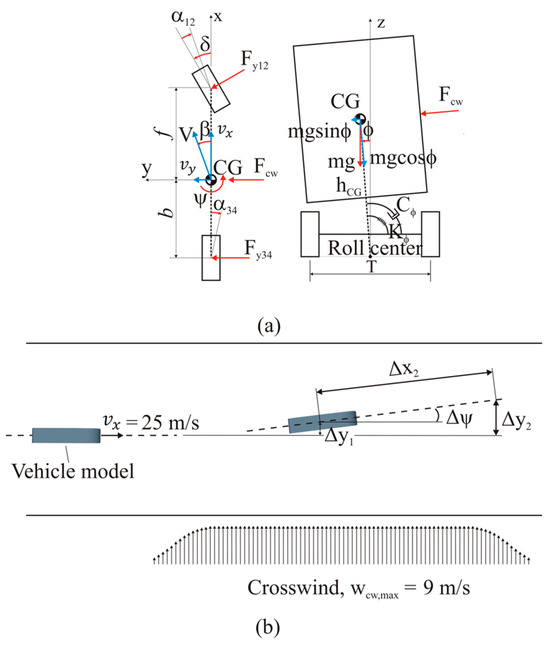
Figure 1.
The graphic representations of (a) the vehicle dynamics model and (b) the simulated vehicle motion in the crosswind.
Equations (1)–(6) provide the equations that govern the dynamics of the vehicle. The vehicle’s longitudinal velocity was set at 25 m/s. Utilizing a linear tire model, both front and rear tyre forces, and , were calculated. The symbols, , , and , respectively, stand for the aerodynamic roll moment, yaw moment and lateral force that crosswind applies to the vehicle. The qualitative descriptions of , , and are given in Figure 2. The other details of the parameters in Equations (1)–(6) are given in Table 1. The effects of suspension moment as a resistance to the body roll motion were represented by the suspension roll stiffness, , and damping, , components in the vehicle model.
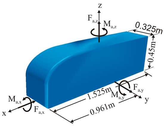
Figure 2.
A descriptive explanation of the aerodynamic forces and moments as well as the geometric features of the Ground Transportation System (GTS) [22] vehicle model. , , , and , , are aerodynamic forces and moments in x-, y- and z-directions, respectively.

Table 1.
Features of the vehicle employed in the study.
In Equation (1), is the steering angle and the other parameters, e.g., and C, are explained in Equations (2)–(6).
2.1.1. Driver Model
The driver model utilized in the current investigation was derived from the research conducted by Winkler et al. [21], in which the crosswind response of a bus was investigated. They modified the constants for proportional gains provided by Wanner et al. [17] to suit the geometry of a bus based on vehicle dynamics data for the bus using the wheel angle, , computed via the understeer gradient, Kus, the curvature radius, R, and the length of the wheelbase, Lwb, with the assumptions of linear tyre behaviour and no-load transfer. Equation (7) provides the driver model, including proportional gain parameters for preview lateral distance, , yaw angle, , and .
The driver’s steering input is denoted by in Equation (7). Additionally, , , are the preview lateral distance, yaw angle, and change in lateral displacement of the vehicle, respectively. Computations of and were determined during the solution of vehicle dynamics equations. Additionally, the calculation of the preview lateral distance, , was based on the assumption of a one-second preview time, resulting in a length of 25 m, considering a longitudinal velocity of 25, as illustrated in Figure 1. Thus, was utilized to calculate the preview lateral distance.
Sets of constants for proportional gains, which were employed to represent three different drivers’ attitudes, are given in Table 2. The first set of constants, denoted as Driver 1, were the proportional gains in the driver model utilized in the study of Winkler et al. [21]. The values of the constants in other sets, i.e., Driver 2 and Driver 3, were proportionally increased relative to the constants in their preceding sets. Therefore, the driver became more skilled as the number of drivers increased. In other words, Driver 1 represented the least skilled driver, Driver 2 represented the more skilled driver than Driver 1, and Driver 3 represented the most skilled driver in the study.
Table 2.
Sets of proportional control gain parameters indicate three different driver’s attitudes.
2.2. Aerodynamics
Incompressible, unsteady Navier-Stokes and continuity equations were used for the solution of turbulent flow around the vehicle. Several approaches are available for the solution of the governing equations of turbulent flows. These approaches include directly solving all flow scales, e.g., direct numerical solution (DNS), modelling all or certain scales of flow, e.g., Reynolds-averaged Navier-Stokes (RANS) and Large Eddy Simulation (LES), or approaches using hybrid RANS-LES methods, e.g., detached eddy simulation (DES). The search for less computationally expensive yet sufficiently accurate methods for solving turbulent flows around vehicles remains a critical need [23,24,25]. For that purpose, hybrid RANS-LES methods, such as DES, were proposed, in which elements of both RANS and LES were combined to provide a balance between computational efficiency and accuracy in simulating turbulent flows. In DES, the simulation dynamically switches between RANS and LES in different regions of the flow, allowing for a more accurate representation of turbulent phenomena. Specifically, RANS is utilized in regions where the flow is predominantly attached and steady, while LES is employed in areas with unsteady and separated flow. However, due to some disadvantages of DES, such as its grid sensitivity in boundary layers and log-layer mismatch, new methods named delayed detached eddy simulation (DDES) and improved delayed detached eddy simulation (IDDES) were proposed [26]. IDDES integrates DDES with an enhanced RANS-LES hybrid model, specifically designed to address wall modelling in LES by adapting to grid resolution [27]. Additionally, Tunay et al. [7] stated that studies employing two-way coupling between aerodynamics and vehicle dynamics in the previous literature commonly utilized scale-resolving turbulence models such as LES and IDDES in aerodynamic simulations, known for their accuracy in turbulent flow solutions compared to RANS equations. Therefore, in the present study, IDDES was used to solve the turbulent flow around the vehicle model.
The Ground Transportation System (GTS), a 1/8-scaled simplified heavy vehicle model, was utilized [22]. Numerous studies [21,22,28,29,30,31] confirmed the applicability of GTS in aerodynamic studies of heavy vehicles. Figure 2 provides the features of the GTS, including the coordinate system, along with qualitative descriptions of aerodynamic force and moments.
The computations utilized a deterministic crosswind velocity profile characterized by a cosine inlet and exit profile with a flat top, as depicted in Figure 3. The mathematical formulation of the crosswind’s velocity profile is defined in Equation (8).
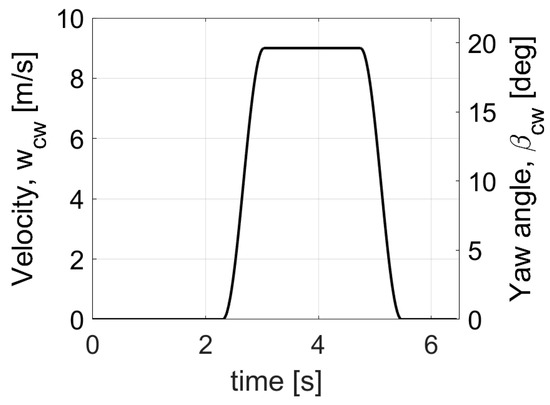
Figure 3.
Velocity profile of the crosswind.
In this instance, the crosswind’s maximum velocity magnitude is indicated by , the length of the transient inlet and exit sections of the crosswind are denoted by , equivalent to 1.5 times the GTS’s length. The symbol, , signifies the distance between the crosswind’s starting location and the origin of the coordinate system, while represents the crosswind’s length, set at five times the GTS’s length. As illustrated in Figure 4a, utilizing a velocity inlet boundary condition on the right-hand side of the flow domain brought the crosswind into computation.
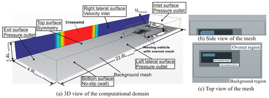
Figure 4.
(a) The computational flow domain in three dimensions and (b,c) view of the mesh structure surrounding the GTS and the overset mesh, respectively. Colours on the right lateral surface of the flow domain represent the profile of the velocity inlet; such as blue indicates zero velocity and red indicates the maximum velocity of 9 m/s.
Figure 4 provides the geometric details of the flow domain, the corresponding computational boundary conditions, and the mesh used in the aerodynamics simulation. The pressure outlet boundary condition was applied to the inlet, outlet, and left lateral surfaces, assuming atmospheric pressure on these boundary surfaces. No-slip boundary conditions were applied to the GTS surfaces and the flow domain’s ground. In addition, the symmetry boundary condition was applied to the top surface of the flow domain. The velocity of the GTS was m/s. Overset mesh was utilized to let the motion of the GTS in the computational domain. The flow had the Reynolds number of , calculated using GTS width. Prior to being used in the vehicle dynamics calculations, the force and moment data from the aerodynamics simulation were scaled back.
StarCCM+ version 13.02 [32], the commercial computational fluid dynamics (CFD) software, was utilized for mesh generation and the solution of the governing equations. As shown in Figure 4, the mesh structures comprised two regions: an overlap region and a background region. The sizes of the overlap region were 5.3 × 2.6 × 1 vehicle lengths, while the background mesh was 22.6 × 4.9 × 1.4 vehicle lengths. The mesh comprised unstructured hexahedral cells totalling approximately 22 million, with approximately 40% (9 million) specifically utilized in the vicinity of the vehicle model, i.e., the overlap region. Twenty prism layers with a total thickness in the wall-normal direction of 0.0141 m, stretching of 1.25 m, and length of 0.0044 m were applied in order to resolve the boundary layer around the GTS. The dimensionless wall distance, y+, was maintained at a value less than 15.
In the current investigation, the GTS’s drag coefficient, CD, in the absence of a cross was 0.251. This number was reasonably close to the numerical and experimental values reported in the literature. For instance, at Rew = 1.6 × 10⁶, the CD values found in the experimental investigations by Croll et al. [28] and Storms et al. [29] were 0.247 and 0.249, respectively. Additionally, the CD value obtained in the numerical study of Unaune et al. [30] at Rew = 2 × 10⁶ was 0.253. Also, the mesh used in this investigation was the same as the mesh used in Winkler et al.’s [21] work, which also looked into the impact of crosswind on the GTS. As a result, it was decided that the mesh was suitable, and no more refinement was done.
The finite volume approach and segregated solver were utilized in the aerodynamic simulations. Convective discretization of the governing equations was accomplished using a hybrid-bounded central differencing (BCD) scheme. For time discretization, a second-order implicit unsteady scheme was employed. The resulting scalar system of equations was solved with a linear solver called Algebraic Multigrid (AMG). In the simulation, a time step of 6 × 10⁻⁵ s was employed, and within each time step, the computation involved five inner iterations.
2.3. Coupled Simulation
By exchanging the force and moment results of the aerodynamics simulation with the vehicle dynamics simulation and the velocity results of the vehicle dynamics simulation with the aerodynamics simulation at each computational time step, a two-way coupling between aerodynamics and vehicle dynamics was achieved. These coupled simulations were executed using high-performance computers (HPC) at the PDC Centre for High-Performance Computing, hosted by the KTH Royal Institute of Technology. The computations utilized 24 nodes with 768 cores.
3. Results
This section provides the study results in three distinct parts. Firstly, the impact of three different drivers’ steering inputs on the vehicle’s response to crosswind disturbances is detailed. Subsequently, the second part delves into the effects of the delay time, tδ,delay, in the drivers’ steering inputs on the vehicle’s response to crosswind. Lastly, the third part elucidates the effects of various drivers’ steering inputs on the characteristics of aerodynamic forces and moments exerted by crosswind on the vehicle.
3.1. The Effects of Drivers’ Steering Inputs with Different Driving Skills on the Vehicle’s Reaction to the Crosswind
Figure 5 presents the comparisons between the vehicle dynamics results obtained with three drivers, each possessing different driving skills and identified as Driver 1, Driver 2, and Driver 3 in the study. These results are juxtaposed with those obtained without any driver’s steering input. As explained previously in Section 2.1.1, Driver 1 represented the least skilled driver, while Driver 3 represented the most skilled driver in the study. Additionally, in this part of the study, after the onset of the crosswind, i.e., tcw,start = 2.67 s, all drivers’ steering inputs began with a delay of tδ,delay = 0.5 s. The crosswind ceased at tcw,end = 5.1 s. The simulation without a driver’s steering input was finished at t = 6.45 s, whereas the simulations with a driver’s steering input were continued until t = 10 s. Aerodynamics and vehicle dynamics simulations were coupled in two-way until t = 6.45 s for both cases, including and not including the driver’s steering inputs.
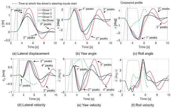
Figure 5.
Comparison of the vehicle dynamics results of three drivers with different driving skills and without any steering input from the driver.
The greatest variations between the lateral displacement results for all drivers occurred at their first peaks, as shown in Figure 5a, i.e., the maximum lateral displacement of Driver 1 is about 1.53 times larger than that of Driver 3. Moreover, the greatest variations between the other results, e.g., yaw and roll angles, happened at their second and third peaks, as shown in Figure 5b,c. Figure 5 indicated that the patterns of yaw angle and lateral displacement findings exhibited a reversal after the initiation of drivers’ steering inputs, in contrast to the results obtained without any steering input from the driver. On the contrary, the drivers’ steering inputs caused the roll angle results to have the same trends as the results obtained without any steering input from the driver. Moreover, the introduction of drivers’ steering inputs led to an increase in the absolute maximum magnitudes of the roll angle results, in contrast to the results obtained without any steering inputs from the driver. Additionally, as expected, the magnitudes of the oscillations observed in the vehicle dynamics results after the crosswind ceased were the least in the results of Driver 3, who is the most skilled in the simulations.
Figure 6 compares the percentage variations, , between the results obtained with steering inputs from the driver and without any steering input from the driver in the first = 0.5 s period after the steering inputs started. The lateral displacement results given in Figure 6 showed larger differences than the roll and yaw angle results at the beginning, i.e., 2.5% at tδ = 3.35. However, the differences in the lateral displacement results showed less increase than the corresponding differences in the roll and yaw angle results at a later instant, e.g., at t = 3.57 s. On the other hand, the percentage variations between the roll angle results obtained with steering inputs from the driver and without any steering input from the driver were larger than those of lateral displacement and yaw angle at the end of this period of the steering inputs, which was 15%. Moreover, the discrepancies among the outcomes of drivers with varying skill levels increased significantly after t = 3.5 s.
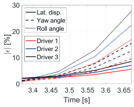
Figure 6.
Percentage variations between the results of the simulations with and without drivers’ steering inputs in the first 0.5 s after the steering inputs start, i.e., tδ,start = 3.17.
Figure 7 shows the steering inputs of three different drivers to the vehicle exposed to crosswind. As presented in Figure 7a, the maximum magnitude of the driver’s steering inputs at their initial peaks increased with an escalation in their driving skills. However, this situation reversed at subsequent peaks, e.g., at the second and third peaks. For example, Driver 3, i.e., the most skilled driver, had the fewest total steering inputs, whereas Driver 1, i.e., the least skilled driver, had the most total steering inputs; see also Figure 8. Figure 7b presents the breakdown of the steering inputs into their proportional gains. Their results showed that there were time shifts between the contributions of the proportional gains. It is expected that a time shift or phase delay between the gains of proportional control might lead to several undesired effects on the control system, e.g., instability and reduced performance. However, in the present situation, the time shifts between the proportional gains, especially the gains from the lateral displacement and the yaw angle, compensated for each other, which caused the reduced amount of steering to bring the vehicle back on its original track. Additionally, as presented in Figure 7c, the maximum steering wheel rate after the first steering manoeuvres of all drivers was smaller than = 240 deg/s. Here, the steering wheel angular velocity was calculated by taking the time derivative of the steering angle at the tyres multiplied by a steering gear ratio of 20.
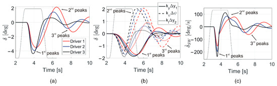
Figure 7.
(a) The steering inputs of three drivers, δ, who had different driving skills, to the vehicle exposed to crosswind. (b) The decomposition of the steering inputs in their proportional gains. (c) The steering wheel angular velocity, .
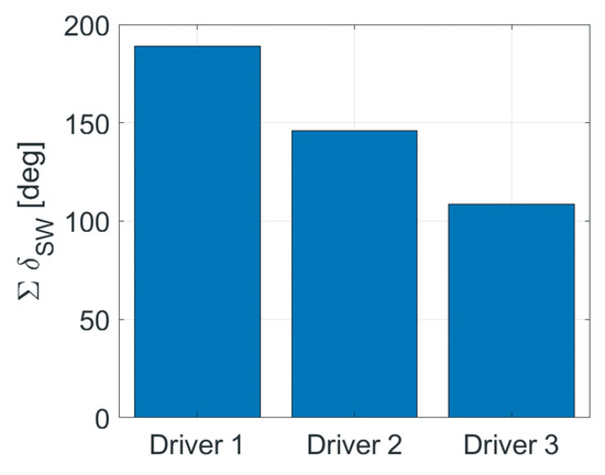
Figure 8.
Total steering wheel input, , of three drivers with different driving skills.
Figure 8 estimates the steering efforts of drivers by integrating the absolute value of the steering wheel angle over the simulation. According to the data shown in Figure 8, the steering effort of Driver 1, who was the least skilled driver in the study, was around 1.7 times the steering effort of Driver 3, who was the most skilled driver in the study.
The temporal evolution of lateral acceleration and yaw velocity in relation to the drivers’ steering inputs is depicted in Figure 9. The delayed correlations between the drivers’ steering inputs and the lateral acceleration and yaw velocity results are exhibited in Figure 9a. Hence, the cross-correlation results between lateral acceleration, yaw velocity, and drivers’ steering inputs, as depicted in Figure 9b, indicated that the vehicle’s yaw velocity responded more promptly to the driver’s steering inputs compared to the vehicle’s lateral acceleration.
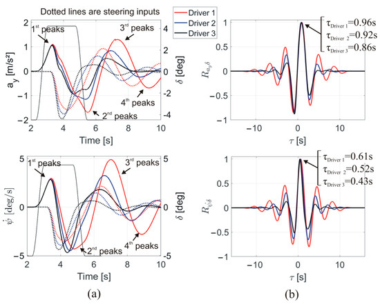
Figure 9.
(a) Comparisons of lateral accelerations, ay, and yaw velocity, , of the vehicle (solid lines) with drivers’ steering inputs, , (dotted lines). (b) Cross-correlations between the lateral acceleration and the steering input by drivers, , and yaw velocity and steering inputs by drivers, .
3.2. The Effects of Time Delay in Drivers’ Steering Inputs on the Vehicle’s Reaction to the Crosswind
In this part of the study, the researchers explored the impacts of delay times in the drivers’ steering inputs on the dynamics of vehicles exposed to crosswind. The lateral displacement, y, yaw angle, , and roll angle, , results of three drivers with different driving skills are presented in Figure 10 at three different delay times, i.e., tδ,delay = 0 s, 0.5 s, and 1.0 s. An ideal steering response time of tδ,delay = 0 s was employed to assess the effects of different delay times in the steering inputs.
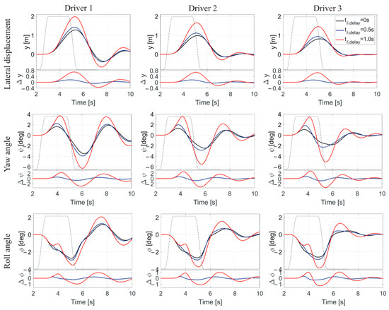
Figure 10.
Lateral displacement, y, yaw angle, , and roll angle, , results of the vehicle obtained in the cases of three delay times, i.e., tδ,delay = 0 s, 0.5 s, and 1.0 s, in the steering inputs of three drivers with different driving skills. The subfigure in each figure shows the instant differences between the results obtained for tδ,delay = 0 s, and tδ,delay = 0.5 s, and 1.0 s.
As the delay time in the drivers’ steering inputs increased, the largest deviations in the yaw angles, roll angles, and lateral displacements of the vehicle due to the crosswind increased. For example, at their initial peaks, the maximum values of the lateral displacements for Driver 1 and Driver 3 at the delay time of tδ,delay = 1.0 s were 1.39 and 1.56 times higher than their respective maximum lateral displacement results at tδ,delay = 0.5 s. On the other hand, the results obtained at tδ,delay = 0 s and 0.5 s were close to each other.
The yaw angle experienced the most significant differences from the delays in drivers’ steering inputs because it had the largest percentage variations between the results obtained at tδ,delay = 0 s and tδ,delay = 1.0 s, as presented in Figure 11. The maximum absolute relative percent difference in the results of the drivers between tδ,delay = 0 s and 1.0 s was at least more than 29%, whereas the highest relative percentage variances in the results of the drivers between tδ,delay = 0 s and 0.5 s were less than 30%. Consequently, the impact of delay time on the vehicle’s response to crosswind disturbances became crucial as the delay time increased from tδ,delay = 0.5 s to tδ,delay = 1.0 s.
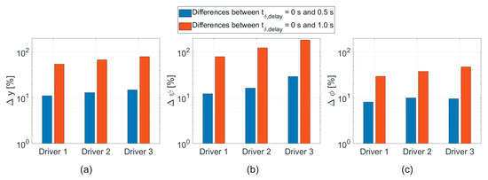
Figure 11.
The highest percentage variations in the (a) lateral displacement, (b) yaw angle, and (c) roll angle results of different drivers between delay times of tδ,delay = 0 s and tδ,delay = 0.5 s and 1.0 s at their first peaks.
Figure 12 depicts the driver’s steering inputs in the instances of three delay times. The magnitudes of the steering inputs of drivers at their initial peaks heightened with both the delay in the steering inputs of drivers and the level of driving skills. For example, the maximum magnitude of the steering input of Driver 3 at the first peak was 1.4 times larger than that of Driver 1 at the delay time of tδ,delay = 1.0 s. Additionally, in the case of Driver 3, the magnitude of the steering input at the first peak at tδ,delay = 1.0 s was around 3 times greater than the corresponding one at tδ,delay = 0 s. Furthermore, the steering efforts needed to bring the vehicle on its original track increased significantly as the delay time in the steering input of the driver increased to tδ,delay = 1.0 s.
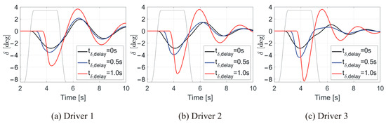
Figure 12.
The steering inputs, δ, of three drivers with different skills at three delay times of tδ,delay = 0 s, 0.5 s, and 1.0 s in the steering inputs.
The total steering wheel inputs of each driver at three distinct delay times are compared in Figure 13. On an individual basis, each driver’s total steering inputs were roughly the same at tδ,delay = 0 s and 0.5 s. Conversely, at tδ,delay = 1.0 s, the total steering inputs of drivers were at least 1.4 times higher than those at tδ,delay = 0 s and 0.5 s. Wagner and Wiedemann [16] specified the importance of the promptness of drivers in controlling the different crosswind sensitivity of vehicles. The findings of the current study unequivocally demonstrated that the delay time of tδ,delay = 0.5 s was important in controlling the vehicle motion after the crosswind hit it. Additionally, there were significant differences between the drivers’ steering inputs. For example, the steering wheel inputs of Driver 1 were 1.7 and 1.3 times larger than those of Driver 3 at tδ,delay = 0 s and 1.0 s, respectively. In conclusion, there were both significant differences between the drivers’ steering inputs at certain delay times and significant increases in the drivers’ steering efforts as the delay time extended to tδ,delay = 1.0 s.
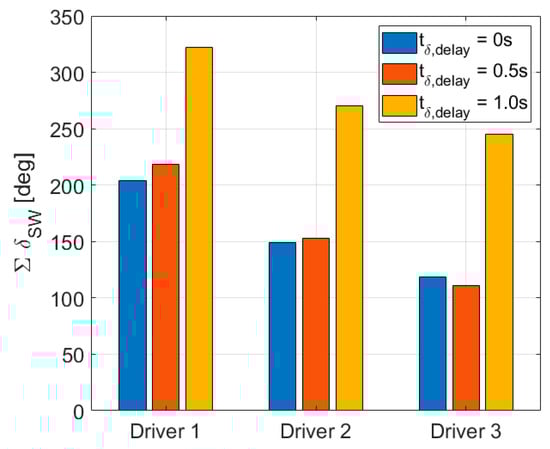
Figure 13.
Total steering wheel inputs of drivers with different driving skills, , at three different delay times, tδ,delay = 0 s, 0.5 s and 1.0 s.
3.3. The Effects of Drivers’ Steering Inputs on the Aerodynamic Force and Moments Acting on the Vehicle Subjected to Crosswind
Previous research studies indicated the significance of the aerodynamic yaw moment, lateral force, and roll moment in influencing the vehicle’s response to crosswind [8,21,33]. The findings demonstrated in the current study revealed that the steering inputs made by the drivers had an impact on the aerodynamic forces and moments acting on the vehicle as a result of the crosswind. The characteristics of lateral force, yaw moment, and roll moment acting on the vehicle due to the crosswind, with and without steering inputs from the driver, are depicted in Figure 14. They revealed that both the drivers’ driving skills and the delay times in their steering inputs caused differences between the aerodynamic forces and moments exerted on the vehicle due to the crosswind. Thus, the differences in the amount of force and moments arose after the steering started, i.e., tδ,delay = 0. For all delay times, the drivers’ steering inputs increased the yaw moment at various amounts towards the end of the crosswind, whereas they reduced the lateral force and roll moment. Rapid alterations in the vehicle’s yaw angle resulting from the drivers’ steering inputs led to notable variations in the yaw moment outcomes. For example, the yaw moment results at tδ,delay = 0 s and 0.5 s reached their maximum values at around t3.9 s, while the yaw moment results at tδ,delay = 1.0 s reached their maximum at a later time of t4.5 s.
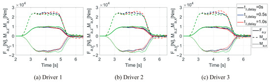
Figure 14.
Lateral force, Fa,y, yaw moment, Ma,z, and roll moment, Ma,x, obtained in the case of three drivers with different skills at three delay times in their steering inputs, i.e., tδ,delay = 0 s, 0.5 s, and 1.0 s. The green lines depict the corresponding forces and moments obtained when there is no driver’s steering input.
Furthermore, the other outcomes of aerodynamics simulation, such as the analysis of velocity fields, were not included in the present study due to the specific scope outlined for this research. However, the detailed analysis of aerodynamics simulation of similar crosswind-vehicle interaction studies can be found in Tunay [6] and Tunay et al. [7,9].
4. Discussion
When investigating the crosswind sensitivity of vehicles, previous research studies often used a traditional approach that ignored the driver’s contributions and concentrated only on the vehicle-crosswind interactions. Wagner and Wiedemann [19] stated that the response of a less crosswind-sensitive vehicle to crosswind might be different when including the driver’s reactions. Thus, in the current study, the responses of a heavy vehicle to a crosswind were investigated by including the steering inputs of three drivers who had different driving skills. Accordingly, the vehicle dynamics results were acquired both with and without the driver’s steering inputs for comparative analysis. Comprehensive discussions regarding the vehicle’s response to crosswind without any driver’s steering input were elaborated in previous studies by Tunay et al. [7,8,9].
When examining the lateral dynamic properties of vehicles, yaw velocity and lateral acceleration and their relationship with steering-wheel angle were generally specified as important characteristics. For instance, Huemer et al. [33] reported that lateral acceleration, yaw velocity, and the time lag between those parameters are the primary factors influencing the driver’s perception of vehicle movements, next to perception limits. In this perspective, the corresponding results are compared in Figure 9, given in the previous section. However, the outcomes presented in Figure 9 demonstrated an intricate interaction among the crosswind, vehicle, and driver’s steering inputs, which made it difficult to compare the results of different driver’s steering efforts and draw any general conclusions regarding them. For example, in Figure 9a, the second peak of the lateral acceleration of Driver 3 occurred inside the crosswind, whereas the second peak of the lateral acceleration of Driver 1 occurred just after the crosswind ceased. That means the larger second peak of the lateral acceleration of Driver 1 could also be due to the reduction in crosswind, not necessarily only due to the steering input. Thus, it is more appropriate to talk about the vehicle-driver system instead of considering their individual effects in the study of the crosswind sensitivity of vehicles [34].
In line with the aim of investigating the driver-vehicle-crosswind interactions, a driver model that reproduced a realistic human driver’s steering response was used in the study. The maximum steering wheel rate after the first steering manoeuvres of all drivers was smaller than = 240 deg/s, given in Figure 7c, indicating that the steering responses of drivers in the study corresponded to normal human driving conditions as described by Blundell and Harty [35] and Wang [36]. Based on empirical observations, Blundell and Harty [35] identified three driving regimes described as “normal”, “spirited”, and “accident avoidance”, which were characterised by steering rates of 0 to 400 deg/s, 400 to 700 deg/s, and 700 to 1200 deg/s, respectively. Also, Wang [36] stated that normal driving requires an average steering rate of 500 deg/s.
In general, the study’s findings indicated that the vehicle dynamics became more stable after the onset of crosswind with higher levels of driver driving skill. The drivers’ steering inputs, aimed at mitigating the unfavourable effects of crosswind on vehicle motion, decreased with increasing driving skills. These outcomes were anticipated, given that the driver model employed in the study was based on proportional gain parameters. However, the variations in the magnitude of the first peaks in the vehicle dynamics results of different drivers were nonlinear, especially in cases where there were time delays, as shown in Figure 10 and Figure 11.
When compared to the outcomes obtained with no steering input, the driver’s initial steering manoeuvre against the crosswind decreased the unfavourable rise in the vehicle’s lateral displacement and yaw angle while increasing the roll angle. The changing rate of the roll angle was the highest in the first 0.5 s of the steering input, whereas the changing rate of the lateral displacement was the lowest. Additionally, the increase in the magnitude of the drivers’ first steering inputs was primarily due to the fast response of the vehicle’s yaw motion to the crosswind disturbances. For example, as presented in Figure 7b, the contributions of the proportional gains obtained from both yaw change, , and the change in the preview lateral distance, , to the first steering manoeuvre of drivers are prompt and higher than the contribution of the change in the lateral displacement, .
Finally, as the results of the on-road crosswind scenario chosen in the study showed, the vehicle’s dynamics, such as lateral displacements, exceeded the acceptable limits set by the road’s lateral margins. This could potentially lead to hazardous situations or accidents.
5. Conclusions
The effects of three different drivers’ steering inputs on the response of a bus to crosswind were investigated. Two-way coupled aerodynamics and vehicle dynamics simulations were employed. The results showed that the maximum lateral displacement of the least skilled driver (Driver 1) was 1.53 times greater than that of the most skilled driver (Driver 3) at tδ,delay = 0.5 s. Additionally, while the level of driving skills increased, the amounts of both lateral displacements and the oscillating motions of the vehicle decreased after the crosswind ceased. The vehicle’s roll angle gave more significant responses to the first steering manoeuvre of drivers than the yaw angle and the lateral displacement.
The effects of delay time in the driver’s steering inputs showed that the delay time of tδ,delay = 0.5 s was important in alleviating the disturbances caused by the crosswind on the vehicle. For example, the vehicle dynamics results obtained in the cases of tδ,delay = 0 s and tδ,delay = 0.5 s were close to each other, whereas the results obtained for tδ,delay = 1.0 s were significantly larger than those of tδ,delay = 0 and 0.5 s. Additionally, the drivers’ total steering inputs at tδ,delay = 1.0 s were at least more than 1.4 times their total steering inputs at tδ,delay = 0.5 s. But each driver’s total steering inputs at tδ,delay = 0.5 s were roughly the same as their total steering inputs at tδ,delay = 0 s. In conclusion, as the delay time increased, the highest percentage variations between the results of different drivers became smaller, but the influence of the long delay time became critical.
Finally, the drivers’ steering inputs increased the yaw moment at various amounts at all delay times towards the end of the crosswind, whereas they reduced the lateral force and roll moment.
Author Contributions
Conceptualization, T.T., L.D. and C.J.O.; methodology, T.T., L.D. and C.J.O.; software, T.T.; validation, T.T., L.D. and C.J.O.; formal analysis, T.T., L.D. and C.J.O.; investigation, T.T., L.D. and C.J.O.; data curation, T.T.; writing—original draft preparation, T.T.; writing—review and editing, T.T., L.D. and C.J.O.; visualisation, T.T.; supervision, L.D. and C.J.O.; funding acquisition, T.T., L.D. and C.J.O. All authors have read and agreed to the published version of the manuscript.
Funding
The authors would like to gratefully acknowledge the co-funding they have received for this work from the Swedish Innovation Agency Vinnova (grant number 2017-03391), the Centre for ECO2 Vehicle Design at KTH (itself funded by Vinnova grant number 2016-05195), and the strategic research area TRENoP. The computations were performed on resources provided by the Swedish National Infrastructure for Computing (SNIC) at the PDC Centre for High-Performance Computing (PDC-HPC).
Institutional Review Board Statement
Not applicable.
Informed Consent Statement
Not applicable.
Data Availability Statement
The data presented in this study are available within the article.
Conflicts of Interest
The authors declare no conflict of interest.
References
- Sims-Williams, D. Crosswinds and transients: Reality, simulation and effects. SAE Int. J. Passeng. Cars. Mech. Syst. 2011, 4, 172–183. [Google Scholar] [CrossRef][Green Version]
- Willumeit, H.P.; Müller, K.; Dödlbacher, G.; Matheis, A. Method to Correlate Vehicular Behaviour and Driver’s Judgement Under Side Wind Disturbances. Veh. Syst. Dyn. 1988, 17, 508–524. [Google Scholar] [CrossRef]
- Lee, S.; Kasahara, M.; Mori, Y. Roll Damping control of a heavy vehicle under the strong crosswind. In Proceedings of the 7th IFAC Symposium on Advances in Automotive Control, The International Federation of Automatic Control, Tokyo, Japan, 4–7 September 2013. [Google Scholar] [CrossRef]
- Trigell, A.S.; Rothhämel, M.; Pauwelussen, J.; Kural, K. Advanced Vehicle Dynamics of Heavy Trucks with the Perspective of Road Safety. Veh. Syst. Dyn. 2017, 55, 1572–1617. [Google Scholar] [CrossRef]
- Juhlin, M.; Eriksson, P.A. Vehicle parameter study on crosswind sensitivity of buses. In Proceedings of the SAE Commercial Vehicle Engineering Congress and Exhibition, Chicago, IL, USA, 26–28 October 2004. [Google Scholar]
- Tunay, T. Two-way coupled aerodynamics and vehicle dynamics simulations of a heavy ground vehicle subjected to crosswind of various frequencies. Proc. Inst. Mech. Eng. D J. Automob. Eng. 2023, 237, 1406–1422. [Google Scholar] [CrossRef]
- Tunay, T.; Drugge, L.; O’Reilly, C.J. Assessment of a Two-Equation Eddy-Viscosity Turbulence Model in Crosswind Simulation of a Heavy Ground Vehicle. SAE Int. J. Commer. Veh. 2022, 15, 81–96. [Google Scholar] [CrossRef]
- Tunay, T.; O’Reilly, C.J.; Drugge, L. The significance of roll on the dynamics of ground vehicles subjected to crosswind gusts by two-way coupled simulation of aero- and vehicle dynamics. In Advances in Dynamics of Vehicles on Roads and Tracks, Lecture Notes in Mechanical Engineering, IAVSD 2019; Klomp, M., Bruzelius, F., Nielsen, J., Hillemyr, A., Eds.; Springer: Cham, Switzerland, 2020. [Google Scholar] [CrossRef]
- Tunay, T.; Drugge, L.; O’Reilly, C.J. On coupling methods used to simulate the dynamic characteristics of heavy ground vehicles subjected to crosswind. J. Wind Eng. Ind. Aerodyn. 2020, 201, 104194. [Google Scholar] [CrossRef]
- Tunay, T.; Drugge, L.; O’Reilly, C.J. Two-way coupled aerodynamics and vehicle dynamics crosswind simulation of a heavy ground vehicle in winter road conditions. In Advances in Dynamics of Vehicles on Roads and Tracks II, Lecture Notes in Mechanical Engineering, IAVSD 2021; Orlova, A., Cole, D., Eds.; Springer: Cham, Switzerland, 2021. [Google Scholar] [CrossRef]
- Brandt, A.; Jacobson, B.; Sebben, S. High speed driving stability of road vehicles under crosswinds: An aerodynamic and vehicle dynamic parametric sensitivity analysis. Veh. Syst. Dyn. 2022, 60, 2334–2357. [Google Scholar] [CrossRef]
- Sekulic, D.; Vdovin, A.; Jacobson, B.; Sebben, S.; Johannesen, S.M. Effects of wind loads and floating bridge motion on intercity bus lateral stability. J. Wind Eng. Ind. Aerodyn. 2021, 212, 104589. [Google Scholar] [CrossRef]
- Zhang, Q.; Su, C.; Zhou, Y.; Zhang, C.; Ding, J.; Wang, Y. Numerical Investigation on Handling Stability of a Heavy Tractor Semi-Trailer under Crosswind. Appl. Sci. 2020, 10, 3672. [Google Scholar] [CrossRef]
- Du, X.; Wang, G. Analysis of Operating Safety of Tractor-Trailer under Crosswind in Cold Mountainous Areas. Appl. Sci. 2022, 12, 12755. [Google Scholar] [CrossRef]
- Liu, H.; Liu, C.; Hao, L.; Zhang, D. Stability Analysis of Lane-Keeping Assistance System for Trucks under Crosswind Conditions. Appl. Sci. 2023, 13, 9891. [Google Scholar] [CrossRef]
- Theissen, P. Unsteady Vehicle Aerodynamics in Gusty Crosswind. Ph.D. Thesis, Technische Universitat München, München, Germany, 2012. [Google Scholar]
- Wanner, D.; Drugge, L.; Edren, J.; Stensson Trigell, A. Modelling and experimental evaluation of driver behaviour during single wheel hub motor failures. In Proceedings of the 3rd International Symposium on Future Active Safety Technology Towards Zero Traffic Accidents (FASTzero’15), Gothenburg, Sweden, 9–11 September 2015. [Google Scholar]
- Drugge, L.; Juhlin, M. Aerodynamic loads on buses due to crosswind gusts: Extended analysis. Veh. Syst. Dyn. 2010, 48, 287–297. [Google Scholar] [CrossRef]
- Wagner, A.; Wiedemann, J. Crosswind behavior in the driver’s perspective. In Proceedings of the SAE 2002 World Congress, Detroit, MI, USA, 4–7 March 2002. [Google Scholar]
- Maruyama, Y.; Yamazaki, F. Driving simulator experiment on the moving stability of an automobile under strong crosswind. J. Wind Eng. Ind. Aerodyn. 2006, 94, 191–205. [Google Scholar] [CrossRef]
- Winkler, N.; Drugge, L.; Stensson Trigell, A.; Efraimsson, G. Coupling aerodynamics to vehicle dynamics in transient crosswinds including a driver model. Comput. Fluids 2016, 138, 26–34. [Google Scholar] [CrossRef]
- Gutierrez, W.T.; Hassan, B.; Croll, R.H.; Rutledge, W.H. Aerodynamics overview of the ground transportation systems (GTS) project for heavy vehicle drag reduction. In Proceedings of the SAE International Congress and Exposition, Detroit, MI, USA, 26–29 February 1996. [Google Scholar]
- Aultman, M.; Wang, Z.; Auza-Gutierrez, R.; Duan, L. Evaluation of CFD methodologies for prediction of flows around simplified and complex automotive models. Comput. Fluids 2022, 236, 105297. [Google Scholar] [CrossRef]
- Chode, K.K.; Viswanathan, H.; Chow, K.; Reese, H. Investigating the aerodynamic drag and noise characteristics of a standard squareback vehicle with inclined side-view mirror configurations using a hybrid computational aeroacoustics (CAA) approach. Phys. Fluids 2023, 35, 075148. [Google Scholar] [CrossRef]
- Zhang, J.; Guo, Z.; Han, S.; Krajnovic, S.; Sheridan, J.; Gao, G. An IDDES study of the near-wake flow topology of a simplified heavy vehicle. Transp. Saf. Environ. 2022, 4, 1–18. [Google Scholar] [CrossRef]
- Saini, R.; Karimi, N.; Duan, L.; Sadiki, A.; Mehdizadeh, A. Effects of NearWall Modeling in the Improved-Delayed-Detached-Eddy-Simulation (IDDES) Methodology. Entropy 2018, 20, 771. [Google Scholar] [CrossRef]
- Shur, M.L.; Spalart, P.R.; Strelets, M.K.; Travin, A.K. A hybrid RANS-LES approach with delayed-DES and wall-modelled LES capabilities. Int. J. Heat Fluid Flow 2008, 29, 1638–1649. [Google Scholar] [CrossRef]
- Croll, R.H.; Gutierrez, W.T.; Hassan, B.; Suazo, J.E.; Riggins, A.J. Experimental investigation of the ground transportation systems (gts) project for heavy vehicle drag reduction. In Proceedings of the SAE International Congress and Exposition, Detroit, MI, USA, 26–29 February 1996. [Google Scholar]
- Storms, B.L.; Ross, J.C.; Heineck, J.T.; Walker, S.M.; Driver, D.M.; Zilliac, G.G. An Experimental Study of the Ground Transportation System (GTS) Model in the NASA Ames 7-by 10-ft Wind Tunnel. NASA TM-2001-209621, 1 February 2001. [Google Scholar]
- Unaune, S.V.; Sovani, S.D.; Kim, S.E. Aerodynamics of a Generic Ground Transportation System: Detached Eddy Simulation. In Proceedings of the 2005 SAE World Congress, Detroit, MI, USA, 11–14 April 2005. [Google Scholar]
- Ghuge, H. Detached Eddy Simulations of a simplified Tractor-Trailer Geometry. Master’s Thesis, Auburn University, Auburn, AL, USA, 2007. [Google Scholar]
- CD-Adapco Inc. STAR-CCM+ 11.0 User Guide; CD-Adapco Inc.: Melville, NY, USA, 2016. [Google Scholar]
- Huemer, J.; Stickel, T.; Sagan, E.; Schwarz, M.; Wall, W.A. Influence of unsteady aerodynamics on driving dynamics of passenger cars. Veh. Syst. Dyn. 2014, 52, 1470–1488. [Google Scholar] [CrossRef]
- Cioffi, A.; Prakash, A.R.; Sabbioni, E.; Vignati, M.; Cheli, F. Heavy-Vehicle Response to Crosswind: Evaluation of Driver Reactions Using a Dynamic Driving Simulator. Vehicles 2023, 5, 344–366. [Google Scholar] [CrossRef]
- Blundell, M.; Harty, D. The Multibody Systems Approach to Vehicle Dynamics, 2nd ed.; Butterworth-Heinemann: Coventry, UK, 2015. [Google Scholar]
- Wang, H. Robust Control for Steer-by-Wire Systems in Road Vehicles. Ph.D. Thesis, Swinburne University of Technology, Melbourne, Australia, 2013. [Google Scholar]
Disclaimer/Publisher’s Note: The statements, opinions and data contained in all publications are solely those of the individual author(s) and contributor(s) and not of MDPI and/or the editor(s). MDPI and/or the editor(s) disclaim responsibility for any injury to people or property resulting from any ideas, methods, instructions or products referred to in the content. |
© 2023 by the authors. Licensee MDPI, Basel, Switzerland. This article is an open access article distributed under the terms and conditions of the Creative Commons Attribution (CC BY) license (https://creativecommons.org/licenses/by/4.0/).