Computer Vision Techniques for Growth Prediction: A Prisma-Based Systematic Literature Review

Abstract

Growth prediction technology is not only a practical application but also a crucial approach that strengthens the safety of image processing techniques. By supplementing the growth images obtained from the original images, especially in insufficient data sets, we can increase the robustness of machine learning. Therefore, predicting the growth of living organisms is an important technology that increases the safety of existing applications that target living organisms and can extend to areas not yet realized. This paper is a systematic literature review (SLR) investigating biological growth prediction based on the PRISMA 2020 guidelines. We systematically survey existing studies from 2017 to 2022 to provide other researchers with current trends. We searched four digital libraries—IEEE Xplore, ACM Digital Library, Science Direct, and Web of Science—and finally analyzed 47 articles. We summarize the methods used, year, features, accuracy, and dataset of each paper. In particular, we explained LSTM, GAN, and STN, the most frequently used methods among the 20 papers related to machine learning (40% of all papers).

1. Introduction

Animal identification recognition in computer vision is the process of estimating the individual from images or videos. It provides rich information about various applications, such as the prevention of damage related to agriculture and forest, ecology investigation, and behavior analysis. Since the enormous economic damage caused to animals covered by the Marine Mammal Protection Act, the identifying technique of the offending individuals are particularly important from the perspective of balancing ecological diversity and economic growth. Identification of individual animals poses a different problem from the usual image classification because the physical characteristics of the same individual can change significantly over time, such as horn growth, injuries, and body defects due to fighting. Animal identification techniques encompass various methods for distinguishing individuals, such as those based on the nose [1,2,3,4], which exhibits minimal change in physical characteristics, differentiation through gait analysis [5,6,7], and identification using tags [8,9,10].

However, it is difficult to photograph animals from the front or without obstacles, as in the case of muzzle-print identification. This circumstance raises the issue of maintaining the quality of the dataset and the possibility of overfitting due to the small number of samplings in the dataset [11,12]. The efficacy and reliability of machine-learning-based individual recognition techniques can improve to accommodate images with various changing physical characteristics, such as multiangle and nighttime images. Metamorphic Testing (MT) increases reliability by adding realistic noise to the image, including weather changes [13,14]. There are many examples of using Generative Adversarial Networks (GANs) to synthesize scenes with various situations and conditions in MT [13,15,16,17]. We also anticipate that our ongoing research explores the possibility of improving the effectiveness and reliability of MT by incorporating a GAN-based technique to address issues related to changing body features, such as horn growth and injuries.

In this paper, we extracted 47 articles from databases such as IEEE Xplore, ACM Digital Library, Science Direct, and Web of Science to predict biological growth using neural networks using a systematic literature review (SLR) method. The SLR methodology is accessed from an electronic database, enabling cross-disciplinary and exhaustive analysis of related issues. SLR studies can be reproducible, ensuring objectivity and transparency.

Section 1 of the paper provides an overview of the topic in the form of an introduction. Section 2 describes the methodology used in this study, including the rationale for conducting an SLR on growth prediction, previous research in this area, the research questions addressed, the search strategy employed, the process of article selection through screening, and the method used to verify the quality of the selected studies. Section 3 of the paper presents the results of SLR method based on the defined research questions. The paper’s discussion is covered in Section 4, while Section 5 concludes the SLR and outlines future directions.

2. Materials and Methods

2.1. Objective

As discussed previously, incorporating physical growth measurements and accounting for changes in climatic and shooting conditions can enhance the robustness and accuracy of machine-learning-based animal identification techniques. This advancement can further establish computer-vision-based identification technology and lead to various applications such as ecological surveys and optimization of capture planning based on behavior prediction, thereby contributing to economics and ecology. For instance, Ella et al. [18] used machine learning to predict the behavior of GPS-tagged animals based on their location data. However, attaching a GPS device to an animal can be burdensome and time-consuming, requiring substantial human resources. By obtaining individual identification data from images and arranging appearance points into time series data, simulation experiments on animal behavior can be conducted based on the research findings of Ella et al.

However, we could not find any studies using machine learning for identification, such as predicting antler growth in deer or cattle. Here raises the question: is it possible to use neural networks (NNs) to predict the growth of living organisms? In other words, the primary motivation of this paper is to investigate existing studies that predict the growth of organisms, with the ultimate goal of increasing the reliability of animal identification through the realization of machine learning techniques.

2.2. Related Works

Some recent literature reviews have dealt with animal identification problems. Hossain et al. (2022) [19] presented an extensive literature review on the problem of cattle identification using machine learning (ML) or deep learning (DL) approaches in the form of an SLR. They discussed the datasets used in ML and DL and classified them by size, pedigree, dataset size, features, feature extraction methods, and performance ratios. However, they did not mention the changes in cattle’s physical characteristics, nor are such papers introduced in that SLR. Kumar et al. (2020) [20] systematically evaluated cattle identification techniques, including machine learning approaches and computer vision (CV) in general, to categorize the techniques as permanent animal identification, semipermanent, and temporary. Vidal et al. (2021) [21] introduced techniques related to CV-based deep learning for individual identification adapted to various animals. They discussed the implications for biology, including ecology, ethology, neuroscience, and conservation modeling. They discussed metric learning, explaining triplet loss as a representative loss function.

There are systematic literature review papers focused on “growth prediction.” T. V. Klompenburg et al. (2020) [22] used search terms such as [“machine learning” AND “yield prediction”] from six electronic databases, including Scopus. They introduced machine learning techniques based on image input and various sensor data such as temperature and other calculated parameters. However, these articles were not included for yield predictions to generate image predictions of growing plants. The study by Taves et al. (2022) [23] is an SLR on Generative Adversarial Network (GAN) and brain images and a comprehensive survey of various GAN techniques. They searched the strings: “(Brain Imaging) OR (Brain Images)” AND “GAN OR Generative Adversarial Network” in two electrical databases. Although this paper painstakingly summarizes growth prediction by GANs, we wanted to know how the growth prediction of CV has been applied in the fields other than brain medicine (e.g., horn growth, plant growth). Table 1 gives the summary of prior research in biological growth prediction.

Table 1. Prior research in biological growth prediction.

Ref. No.	Year	Objective	Type
[22]	2020	This paper summarizes machine learning approaches to yield prediction.	SLR
[23]	2022	This paper summarizes generative adversarial network in brain imaging.	SLR (PRISMA)
[24]	2020	This paper discusses various crop growth modeling approaches.	overview
[25]	2022	This paper describes remote sensing techniques based on data acquisition requirements for deep learning in crop yield prediction.	SLR (PRISMA)

2.3. Methodology

We developed a review protocol referred to the Preferred Reporting Items for Systematic Reviews and Meta-Analysis (PRISMA) guidelines [26], as shown in Figure 1. This guideline first defines the research question (RQ). Then, we conducted preliminary research and developed a strategy for the databases and search terms. Next, we performed a step-by-step selection process for the obtained papers: exclusion based on abstract and title (step 1) and selection based on exclusion criteria (step 2). In the quality verification part, the authors verified the extracted papers’ validity and the extraction result’s reproducibility. In the final part of the guideline, we extracted data from the documents to solve the RQ, visualize the data, and explain important terms and papers.

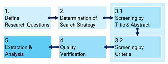
Figure 1. Steps in the formulated review protocol.

2.4. Research Questions (RQ)

At first, RQ is strictly defined according to the PRISMA guideline. We were initially interested in the applicability and accuracy of machine learning to antler growth prediction to improve the identification problem’s accuracy. However, there have yet to be any articles that are applied machine learning methods for antler growth. Not just for our research, image processing technology for biological growth prediction is one of the critical issues for every researcher and practitioner to improve the robustness of learning. We have yet to discover a technique for simulating deer antler growth. Still, we must investigate whether image growth prediction can apply to various fields in initiating research on MT. Though previous articles (Table 1) have done SLR, we found that their studies reveal the following limitations:

• There needs to be an extensive review of which subjects can predict image growth.
• Some papers summarize growth prediction in several applications using machine learning but need a mathematical explanation.

Based on the above considerations, we defined the RQ in Table 2.

Table 2. This table summarizes the research questions and what can be accomplished by those resolutions.

Index	Research Questions	Goal
RQ1	What is the purpose of using computer vision (CV) to predict the growth of organisms?	The report clarifies areas of application that have been applied already and identifies the potential for development into other applications.
RQ2	Which technologies are used for growth prediction using image processing?	The integration results will identify what machine learning techniques, or non-machine learning techniques, are effective.
RQ3	What are the specific details of these technologies for growth prediction using image processing?	We will indicate recent research trends by extracting the distribution of datasets, software, features, accuracy, and years.
RQ4	Which mathematical models can be used to explain the machine learning models employed for growth prediction?	This question leads to a well-organized understanding of trends and differences in machine learning models.

2.5. Determination of Search Strategy

We considered search terms that would produce results satisfying the RQs in Table 2. We searched for “growth prediction” in four electronic databases (ACM Digital Library, IEEE Xplore, Science Direct, and Web of Science) from 1 January 2017 to 31 December 2022. We identified our search terms by progressively increasing the number of words for searches on biological growth with external changes, as shown in Figure 2. This study initially searched for (“GAN” AND “growth prediction”) and analyzed keywords and trends in some extracted articles. In some cases, searching for the same queries in all electronic databases yields many results, so each database’s search queries are changed in detail. As a result, the available search strings were (“growth” AND “prediction” AND “imaging”). Different search strings were used depending on the search function of each of the four databases (January 2023). The search strings for the databases are shown in Table 3.

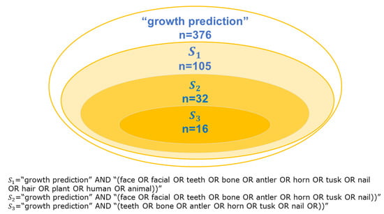
Figure 2. Inclusion of search results obtained with terms searched in Web of Science.

Table 3. Search strings for 4 databases (IEEE Xplore, ACM Digital Library, Science Direct and Web of Science).

Journal	Queries
IEEE Xplore	(“All Metadata”:“growth” AND “All Metadata”:“prediction” AND “All Metadata”:imaging) AND (“All Metadata”:“horn” OR “All Metadata”:“plant” OR “All Metadata”:“antler” OR “All Metadata”:“tusk” OR “All Metadata”:“face” OR “All Metadata”:“tumor” OR “All Metadata”:“cell” OR “All Metadata”:“octopus” OR “All Metadata”:“starfish” OR “All Metadata”:“human” OR “All Metadata”:“age” OR “All Metadata”:“animal”) NOT (“IEEE Terms”:“image segmentation”) NOT (“IEEE Terms”:“recognition”)
ACM Digital Library	((Keywords: gan) OR (Keywords: “generative adversarial network”) OR (Keywords: vae) OR (Keywords: “stable diffusion” OR (Keywords: “adversarial auto encoder”) OR (Keywords: aae) OR (Keywords: “spatial transform”)) AND NOT (Keywords: “image segmentation”) AND NOT (Keywords: recognition) AND (All: growth) AND (All: prediction) AND (All: imaging) AND ((All: horn) OR (All: antler) OR (All: face) OR (All: plant) OR (All: tusk) OR (All: bone) OR (All: teeth) OR (All: age) OR (All: human) OR (All: animal) OR (All: nail) OR (All: hair) OR (All: starfish) OR (All: octopus))
Science Direct	“growth prediction” AND “imaging” AND (“horn” OR “antler” OR “tusk” OR “bone” OR “teeth” OR “age”)
Web of Science	“growth prediction” AND (“face” OR “facial OR “teeth” OR “bone” OR “antler” OR “horn” OR “tusk” OR “nail” OR “hair” OR “plant” OR “human” OR “animal”)

2.6. Article Selection by Screening

We screened the articles obtained from the databases according to the PRISMA 2020 guidelines. A flowchart and description of the selection process are provided in Figure 3 and the Appendix. We obtained 536 articles, with 216 from Science Direct, 181 from IEEE Xplore, 105 from Web of Science, and 34 from ACM Digital Library.

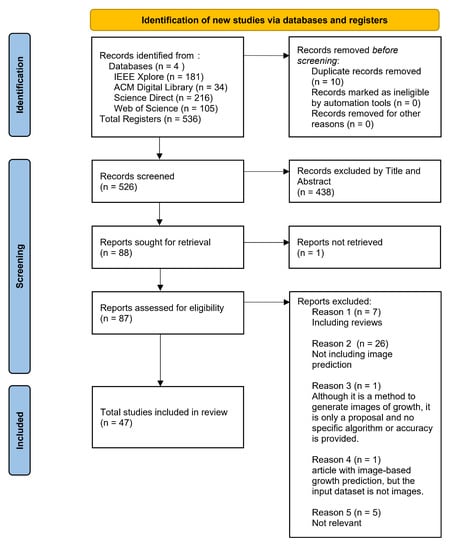
Figure 3. PRISMA 2020 workflow of the identification, screening, eligibility, and inclusion of the studies in the systematic review.

2.6.1. Screening (Step1: Screening by Title & Abstract)

After removing 10 duplicates, 526 articles were retained; we excluded 438 articles by titles and abstract criteria. We automatically removed papers that included segmentation in the keywords and titles because we judged that many articles related to machine learning mainly deal with segmentation and that these papers are not primarily concerned with growth prediction. Also, we automatically removed the articles from the results that included these words: “crack” (21), “fatigue” (20), “urban” (17), “crystal,” and some metal words. Then, we analyzed the full texts of 88 reported studies.

2.6.2. Screening (Step2: Screening by Exclusive Criteria)

We could not obtain Kahala et al. [27] and report it as not eligible, but the summary includes a description of bone growth modeling, which is highly relevant to this SLR. Of the 87 papers, 40 were excluded for the following reasons, and 47 were retained. The first reason was that “the paper is a review” (n = 7), and the second was that “the paper does not include image-based growth prediction” (n = 26).

2.7. Quality Verification

The assessment of bias risk is described in this section. This SLR downloaded the search results from each database in BibTex format, and we performed the selection process by a single person using the Zotero tool. All authors double-checked the results of the sorting to confirm the quality.

3. Results (Extraction & Analysis)

3.1. Rq1: What Is the Purpose of Using CV to Predict the Growth of Organisms?

The selected studies correspond to various applications, which are summarized in Table 4. In this research survey, we searched papers on the horn growth process (for example, deer, buffalo, and snail) and documents describing the regeneration mechanism. However, we tried to find them in the database we used. This fact clarified a critical avenue for the direction and theme of our future research. Therefore, we reconfirmed the significance of this research and found that this topic has great potential for future research.

Table 4. Distribution on the main objectives of growth prediction with computer vision.

Main Objective	Studies, n(%)	Conditions Included
The tumor cellularity	18 (39)	breast cancer (3), Pancreatic neuroendocrine (1), Vertebral tumor (1), Brain tumor (5), Glioma (1), Pancreas (1), Lung cancer (1)
The plant growth	8 (18)	Cauliflower (1), Arabidopsis (1), Forests (1), Komatsuna (3), Butterhead (2), Rice leaf (1), Aberystwyth (2), Arabidopsis Thaliana (1)
The vessel growth	8 (18)	atherosclerotic plaques (3), left circumflex Abdominal Aortic Aneurysm (AAA) (4), coronary artery (1)
The bone morphology	6 (13)	Mandibular (1), Bone implant (1), Femur (2), Scoliosis (1), Spine (1)
The cell growth	2 (5)	Human Pluripotent Stem (1)
The facial Prediction	2 (5)
Geographic Atrophy (GA)	2 (5)
The brain growth	1 (3)

Many studies predicted the growth of parameters directly related to applications, such as biomarkers and leaf area (excluded from this SLR). Tumor cellularity predictions were the most common study, accounting for 39% of the total, followed by plant growth and vascular growth predictions, which accounted for about the same number, about 18%. Bone growth predictions were next, with about 6 studies, which was less than expected. Many studies predicted the growth of parameters directly related to applications, such as biomarkers and leaf area, excluded from this SLR. In contrast to these studies, the number of studies that output image representations was negligible during the survey.

3.2. Rq2: Which Technologies Are Used for Growth Prediction Using Image Processing?

This SLR confirmed that publications increased from 2017 to 2022 (Figure 4). There were 27 submissions on non-machine learning models compared to 20 on machine learning models. In Table 5, we finalize the method used for each article. As explained in later chapters, the top categories of machine learning models were LSTM, GAN, and STN. We consider the increasing number of papers on growth forecasting due to the rise of machine learning models in recent years. In Section 3.4, we explain the above machine learning models.

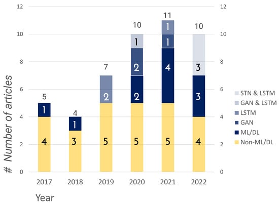
Figure 4. Distribution of publication years 2017–2022.

3.3. Rq3: What Are the Specific Details of These Technologies for Growth Prediction Using Image Processing?

3.3.1. Dataset

In most of the literature, there are few examples of external datasets, and the data are sampled and processed within the study to create the dataset. In this SLR, the only dataset that appears in common is Aberystwyth [28]. This result may be attributed to the sampling environment and ease of preprocessing, such as labeling and segmentation. In addition, as shown in Table 4, more than 80% of the studies are in the medical field, and the datasets are mainly composed of medical data such as “MRI”, “OCT”, “CT”, and “X-RAY’.

3.3.2. Software

Due in part to the recent development of open software in machine learning libraries, the use of ADAM optimizer was used in 7 cases [29,30,31,32,33,34,35], Pytorch in 5 cases [29,33,35,36,37], Numpy in 2 cases [38,39], TensorFlow in 2 cases [30,40], and OpenCV in 2 cases [41,42]. (By considering the mean square and mean of the gradient as first and second-order moments, weights can be updated on an appropriate scale for each parameter.)

Table 5. Studies on growth prediction.

Article	Method Name	Feature	Data Sets	Accuracy	Software Tool	Year
Nino-Sandova et al. [43]	ANN, SVR	17 variables of anatomic relevance	9 landmarks from 229 cephalograms [44]	correlation coefficients = 0.96 (the variables Cd-Go-Gn)	MATLAB	2017
A. Jarret et al. (2020) [45]	PDE	6 variables, 10 parameters	MRI and PET data	-	RapidMiner	2020
Q. Meng et al. [46]	FEM	N + 1 parameters (N = 12)	OCT images of 6 AMD patients	TPR = 82.4 ± 3.4%, FPR = 21.1 ± 2.7%, DC = 81.4 ± 1.6%, RVD = 3.8 ± 3.5% (R group)	COSMOL, MATLAB, LiveLink	2021
L. Drees et al. [47]	cGAN [48]	The loss weighting parameter $\lambda =100$	7618 training and 2707 test pairs	R2 value = 0.95	Pix2Pix	2021
H. Wang et al. [29]	SDC-Transformer, LATM	The final image channel number = 256	15,900 sets of tumor data	RMSE = 11.32 Dice = 89.31%, Recall = 90.57%,	Pytorch framework Adam optimizer for loss optimization	2022
Ling Zhang et al. (2020) [30]	ST-ConvLSTM, BeyondMSE (GAN)	STConvLSTM models for 5 epochs with the batch size of 16	4D longitudinal tumor dataset (33 patients), CETUS [49] (172,296 training subsequences)	Dice score of $83.2\%\pm 5.1$ RVD of $11.2\%\pm 10.8$	TensorFlow Adam optimizer	2020
Jung et al. (2022) [36]	STN, U-Net with two LSTMs	six L1 losses (4 STN losses shape and texture losses)	Aberystwyth [28] (1674 images), Komatsuna (448 images) [50], own Butterhead (972 images)	PNSR (dB) = 30.55, SSIM = 0.9042	PyTorch framework (with 2 NVIDIA RTX 2080ti GPUs)	2022
Jarret et al. (2021) [51]	PDE	6 variable, 8 parameters	DW-MRI and DCE-MRI patient datasets [52]	errors $<17\%$ (total cellularity, volume and longest axis)	REDCap, MATLAB, Elastix	2021
Ghosh et al. (2021) [53]	BPNN, GA	model A (6 parameters), model B (3 parameters), model C (2 parameters)	Results of FE-based mechanoregulatory analysis (80, 52, 36 for each model)	R2 = (0.997, 0.810) MSE = 0.0001 (model B)	CATIA v5R20, ANSYS V14.5 MATLAB	2021
D.S. Pleouras et al. [54]	PDE	8 parameters	CCTA from SMARTool	-	[55,56]	2020
A. I. Sakellarios et al. [57]	The Navier– Stokes equations, Darcy’s Law et al.	4 parameters, 4 parameters	intravascular ultrasound (IVUS) and OCT images	the accuracy in predicting regions potential for athe- rosclerotic plaque develop- ment $R^2=0.847(p=0.009$, adjusted $R^2=0.738)$	Workbench Meshing 14.0, ANSYS CFX 14.0, IBM SPSS Statistics v20	2017
H. N. Do et al. [58]	Gaussian process regression, IS field	The Kalman filter covariance matrix ($n\times n$, n = 64,000)	CT image of 7 subjects (4–7 scans)	Hausdorff distance errors = 6.26	MeshLab	2019
S. nesteruk et al. [41]	Holt-Winters model, autoregression	-	RGB 600 images for every plant	Mean Absolute Percentage Error (MAPE) = 5.6 (4 days)	OpenCV, sklearn, Pandas	2020
T.H Kim et al. [59]	Hierarchical Auto- encoder, STN	the L1 norm (loss function)	RGB 10 Butterhead own datasets	PSNR (dB) = 23.13 SSIM = 0.8221	-	2022
L. Zhang et al. [60]	synthetic G & R model, Bayesian calibration m- ethod	${\theta }_1=0.05,0.2,0.35,$ ${\theta }_2=0.7,0.90,0.99$ in real observation	CT scan images (3 patient)	prediction error (cm) = 0.0070 (P2, 2.3 year)	GPML in MATLAB 2018	2019
K. Wong et al. [61]	Elastic-growth decomp- osition, FEM	hyperelastic constitutive law	7 patient FDG-PET) images and CT image data sets	Recall = $83.2\pm 8.8\%$, Precision = $86.9\pm 8.3\%$, Dice coefficient $=84.4\pm 4.0\%$, Relative volume differ- ence $=13.9\pm 9.8\%$	Insight Segmentation and Registration Toolkit (ITK)	2017
M.G. Alonso et al. [62]	FEM	4 dimensionless parameters	Standardized femur model	$t^{\prime }=0.33$, $ϵ=5.5\times {10}^{-3}$ $\lambda =21.2$, $\kappa =10\times {10}^4$	Salome-mesh meshing software	2020
Z. Jiang et al. [63]	G & R, HFM, LFM	The patient-specific values of parameters $K_g$ and ${\sigma }_{dmg}$ from follow-up CT images	82 CT images of AAAs from 21 patients	The average prediction error: The diameter = 1.39 mm, Max diameter along centerline = 1.67 mm	MATLAB toolbox, ooDACE	2021
I. Rekik et al. [64]	Enhanced longitudinal multishape prediction algorithm	${\sigma }_W=5$ for the shape kernel $K_W$,${\sigma }_V=30$ for the deformation kernel $K_V$	Longitudinal diffusion and structural MR im- ages (5 infants)	Estimation error (with mean guidance): = 1.64 (3 months)	FSL tools	2017
Y. Wu and H. Zhu [31]	LSTM	7 parameters in LSTM network	Backscatter microwave signal of the breast	RMSE = 0.021, MAE = 0.018, R-squared = 0.946	Kras framework, ADAM optimizer	2019
H. Fouad et al. [65]	HHTGM, GB model	CNNs are used for detecting possible vertebras	cervical and lumbar MR images	98.66% accuracy (HTTGM)	-	2019
W. Mandel et al. [32]	STCN	batch size = 32, learning rate = 0.001, dropout and recurrent drop rate = 0.5	695 3D spine models, 3D spine reconstructions (72 operative patients)	3D RMS $=1.7\pm 0.7$ (mm) Dice $=95.0\pm 2.4\%$	ADAM optimizer	2021
Y-H Chang et al. [42]	RNN, LSTM	6 parameters	107 microscopic images	error rates are almost under 10%	OpenCV, MetaMorph	2019
M. Tajdari et al. [66]	Mechanistic NN	using all the 204 landmarks	X-ray images (train: 856, test: 184)	Relative approximation error = 0.28% (127 months)	ABAQUS	2021
A. Elazab at al. (i) [33]	GP-GAN	generator $G_1,G_2$, discriminator $D_1,D_2$	MRI images from 18 subjects (sampling data and BRATS 2014 dataset)	JI = 78.99%, DC = 88.26%	Pytorch	2020
A. Elazab at al. (ii) [37]	GAN, U-Net	Dice loss, learning rate = 0.001, weight decay = 0.9 and 0.999	MRI Images from 9 subjects	JI = 76.51%, DS = 86.68%	Pytorch, ADAM optimizer	2020
K. scheufele et al. [67]	PDE	-	mpMRI images (206 GBM patients from BraTS’18)	CV avg-accuracy $=0.52\pm 0.12$	CLAIRE	2021
Y. Meng et al. [34]	CGRU	Generative Adversarial loss, learning rate = 0.0001, The batch size = 4	KOMASTUNA plant images [28]	RGB avg-PSNR = 26.55 instance masks PSNR = 26.92	AdamW optimizer	2022
S. Haung et al. [38]	$F^3$	FLM, FVS, FIA	305 FIA plot (2003–2014), Landsat 5 Thematic Mapper (TM) images, etc.	RMSE = 12.89 MAE = 8.5	Fortran Python (arcpi, scipy, numpy, etc.)	2018
J-H. Moon et al. [68]	PLS	161 predictor variables	Serial longitudinal lateral cephalograms (303 children)	prediction error 0.03 mm/y, Exact RMSE and MSE values are unknown (only figure)	R language	2022
H. Matthews et al. [69]	PLSR	-	3D surface sampling: 28,861	Exact RMSE values is unknown (only figure)	Mevislab	2018
H. Kainz et al. [70]	FEM	-	motion capture data of 22 children	average (standard deviation): $0.{34}^{\circ }\left(0.09\right)$ are decrease	-	2021
S. Subramanian et al. [71]	PDE	NME model ($\gamma =0$)	singletime-point structural mpMRI scans (216 GBA patients)	(TC, VT) dice scores = (0.84, 0.527)	[72], MPI	2022
K. scheufele et al. [73]	SIBIA, PDE	-	RTRV real data (6 patient)	Dice score: 93–97%	-	2019
Ling Zhang et al. (2018) [74]	ConvNet	weight decay = 0.0005, momentum = 0.9, mini-batch size = 512, aggressive dropout ratio = 0.9	multimodal image (dual phase contrast-enhanced CT and FDG-PET) for 10 patients	Dice coefficient = $86.8\pm 3.4\%$, RVD = $6.6\pm 7.1\%$	Caffe platform	2018
W. Yi et al. [40]	SVR, CNN	-	709 collected sample RGB data	MSE = 0.156817 (CNN)	OpenGL 3.2, TensorFlow	2020
E. M. Moult et al. [75]	Atrophy front growth model	-	OCT imaging dataset of 38 GA eyes (27 patients)	MSE = 0.156817 (CNN)	absolute error $<0.05$ mm/year	2022
A. Elazab et al. (2019) [76]	Log-kill method	PSO 7 parameters, GM = VM = 694 Pa	8 postsurgical MRI datasets of LGG patients	$JI=0.77-10.05\%$, $DC=1.2-14.47\%$	3D Slicer	2019
Y. Zhang et al. [77]	BiLSTM, 3D-U-net	22 layers in 3D-U-net	SD-OCT projection images (22 patients)	DI = 0.86, CC = 0.83 (avg-mean)	-	2021
L. Wang et al. [78]	QuarterNet, Siamese network	hyper-parameters $w_n=0.6$, $w_p=0.4$, $\lambda =0.2$	CT images of 1413 lung cancer patients	AUC > 0.88	-	2021
T. Kim et al. [35]	hierarchical auto-encoder	L1 norm, initial learning rate = 0.0001	[28,79,80]	PSNR = 30.61 (Aberystwyth leaf), SSIM = 0.9065 (Komatsuna)	Pytorch, ADAM optimizer	2022
K. Malavazos [81]	multi compartmental continuum approaches	-	RIDER-NEURO MRI images database [82]	Accelerator Efficiency = 28.4	-	2020
H. Dong et al. [83]	UFD model	6 parameters	4 patient CT images	The mean node-to- surface distance: 0.04–0.09 mm (Psot 2)	MATLAB 2018b, Abaqus FEA 2020	2022
M. M. Rahman et al. [84]	3D tissue scale model, Agent-based cellular scale model	20 paramaters	10 days observed images by MRI	mean of the relative errors < 1.0 %	COMSOL	2017
T. Roque et al. [85]	PDE	-	DCE-MRI images	volume errors (<5%), Dice overlaps (>97%)	MATLAB	2018
D. Pleouras et al. [86]	Navier-Stokes equations	-	CCTA images (60 patients)	$r^2=0.49$, $p<0.0001.$	-	2019
C. J. Huang et al. [39]	ResNet34, U-net	-	Training images: 1090 Test images: 273	Accuracy: 90.6%	numpy 1.21.0 scikit-learn 0.42.2	2022

Table 5. Studies on growth prediction.

Article	Method Name	Feature	Data Sets	Accuracy	Software Tool	Year
Nino-Sandova et al. [43]	ANN, SVR	17 variables of anatomic relevance	9 landmarks from 229 cephalograms [44]	correlation coefficients = 0.96 (the variables Cd-Go-Gn)	MATLAB	2017
A. Jarret et al. (2020) [45]	PDE	6 variables, 10 parameters	MRI and PET data	-	RapidMiner	2020
Q. Meng et al. [46]	FEM	N + 1 parameters (N = 12)	OCT images of 6 AMD patients	TPR = 82.4 ± 3.4%, FPR = 21.1 ± 2.7%, DC = 81.4 ± 1.6%, RVD = 3.8 ± 3.5% (R group)	COSMOL, MATLAB, LiveLink	2021
L. Drees et al. [47]	cGAN [48]	The loss weighting parameter $\lambda =100$	7618 training and 2707 test pairs	R2 value = 0.95	Pix2Pix	2021
H. Wang et al. [29]	SDC-Transformer, LATM	The final image channel number = 256	15,900 sets of tumor data	RMSE = 11.32 Dice = 89.31%, Recall = 90.57%,	Pytorch framework Adam optimizer for loss optimization	2022
Ling Zhang et al. (2020) [30]	ST-ConvLSTM, BeyondMSE (GAN)	STConvLSTM models for 5 epochs with the batch size of 16	4D longitudinal tumor dataset (33 patients), CETUS [49] (172,296 training subsequences)	Dice score of $83.2\%\pm 5.1$ RVD of $11.2\%\pm 10.8$	TensorFlow Adam optimizer	2020
Jung et al. (2022) [36]	STN, U-Net with two LSTMs	six L1 losses (4 STN losses shape and texture losses)	Aberystwyth [28] (1674 images), Komatsuna (448 images) [50], own Butterhead (972 images)	PNSR (dB) = 30.55, SSIM = 0.9042	PyTorch framework (with 2 NVIDIA RTX 2080ti GPUs)	2022
Jarret et al. (2021) [51]	PDE	6 variable, 8 parameters	DW-MRI and DCE-MRI patient datasets [52]	errors $<17\%$ (total cellularity, volume and longest axis)	REDCap, MATLAB, Elastix	2021
Ghosh et al. (2021) [53]	BPNN, GA	model A (6 parameters), model B (3 parameters), model C (2 parameters)	Results of FE-based mechanoregulatory analysis (80, 52, 36 for each model)	R2 = (0.997, 0.810) MSE = 0.0001 (model B)	CATIA v5R20, ANSYS V14.5 MATLAB	2021
D.S. Pleouras et al. [54]	PDE	8 parameters	CCTA from SMARTool	-	[55,56]	2020
A. I. Sakellarios et al. [57]	The Navier– Stokes equations, Darcy’s Law et al.	4 parameters, 4 parameters	intravascular ultrasound (IVUS) and OCT images	the accuracy in predicting regions potential for athe- rosclerotic plaque develop- ment $R^2=0.847(p=0.009$, adjusted $R^2=0.738)$	Workbench Meshing 14.0, ANSYS CFX 14.0, IBM SPSS Statistics v20	2017
H. N. Do et al. [58]	Gaussian process regression, IS field	The Kalman filter covariance matrix ($n\times n$, n = 64,000)	CT image of 7 subjects (4–7 scans)	Hausdorff distance errors = 6.26	MeshLab	2019
S. nesteruk et al. [41]	Holt-Winters model, autoregression	-	RGB 600 images for every plant	Mean Absolute Percentage Error (MAPE) = 5.6 (4 days)	OpenCV, sklearn, Pandas	2020
T.H Kim et al. [59]	Hierarchical Auto- encoder, STN	the L1 norm (loss function)	RGB 10 Butterhead own datasets	PSNR (dB) = 23.13 SSIM = 0.8221	-	2022
L. Zhang et al. [60]	synthetic G & R model, Bayesian calibration m- ethod	${\theta }_1=0.05,0.2,0.35,$ ${\theta }_2=0.7,0.90,0.99$ in real observation	CT scan images (3 patient)	prediction error (cm) = 0.0070 (P2, 2.3 year)	GPML in MATLAB 2018	2019
K. Wong et al. [61]	Elastic-growth decomp- osition, FEM	hyperelastic constitutive law	7 patient FDG-PET) images and CT image data sets	Recall = $83.2\pm 8.8\%$, Precision = $86.9\pm 8.3\%$, Dice coefficient $=84.4\pm 4.0\%$, Relative volume differ- ence $=13.9\pm 9.8\%$	Insight Segmentation and Registration Toolkit (ITK)	2017
M.G. Alonso et al. [62]	FEM	4 dimensionless parameters	Standardized femur model	$t^{\prime }=0.33$, $ϵ=5.5\times {10}^{-3}$ $\lambda =21.2$, $\kappa =10\times {10}^4$	Salome-mesh meshing software	2020
Z. Jiang et al. [63]	G & R, HFM, LFM	The patient-specific values of parameters $K_g$ and ${\sigma }_{dmg}$ from follow-up CT images	82 CT images of AAAs from 21 patients	The average prediction error: The diameter = 1.39 mm, Max diameter along centerline = 1.67 mm	MATLAB toolbox, ooDACE	2021
I. Rekik et al. [64]	Enhanced longitudinal multishape prediction algorithm	${\sigma }_W=5$ for the shape kernel $K_W$,${\sigma }_V=30$ for the deformation kernel $K_V$	Longitudinal diffusion and structural MR im- ages (5 infants)	Estimation error (with mean guidance): = 1.64 (3 months)	FSL tools	2017
Y. Wu and H. Zhu [31]	LSTM	7 parameters in LSTM network	Backscatter microwave signal of the breast	RMSE = 0.021, MAE = 0.018, R-squared = 0.946	Kras framework, ADAM optimizer	2019
H. Fouad et al. [65]	HHTGM, GB model	CNNs are used for detecting possible vertebras	cervical and lumbar MR images	98.66% accuracy (HTTGM)	-	2019
W. Mandel et al. [32]	STCN	batch size = 32, learning rate = 0.001, dropout and recurrent drop rate = 0.5	695 3D spine models, 3D spine reconstructions (72 operative patients)	3D RMS $=1.7\pm 0.7$ (mm) Dice $=95.0\pm 2.4\%$	ADAM optimizer	2021
Y-H Chang et al. [42]	RNN, LSTM	6 parameters	107 microscopic images	error rates are almost under 10%	OpenCV, MetaMorph	2019
M. Tajdari et al. [66]	Mechanistic NN	using all the 204 landmarks	X-ray images (train: 856, test: 184)	Relative approximation error = 0.28% (127 months)	ABAQUS	2021
A. Elazab at al. (i) [33]	GP-GAN	generator $G_1,G_2$, discriminator $D_1,D_2$	MRI images from 18 subjects (sampling data and BRATS 2014 dataset)	JI = 78.99%, DC = 88.26%	Pytorch	2020
A. Elazab at al. (ii) [37]	GAN, U-Net	Dice loss, learning rate = 0.001, weight decay = 0.9 and 0.999	MRI Images from 9 subjects	JI = 76.51%, DS = 86.68%	Pytorch, ADAM optimizer	2020
K. scheufele et al. [67]	PDE	-	mpMRI images (206 GBM patients from BraTS’18)	CV avg-accuracy $=0.52\pm 0.12$	CLAIRE	2021
Y. Meng et al. [34]	CGRU	Generative Adversarial loss, learning rate = 0.0001, The batch size = 4	KOMASTUNA plant images [28]	RGB avg-PSNR = 26.55 instance masks PSNR = 26.92	AdamW optimizer	2022
S. Haung et al. [38]	$F^3$	FLM, FVS, FIA	305 FIA plot (2003–2014), Landsat 5 Thematic Mapper (TM) images, etc.	RMSE = 12.89 MAE = 8.5	Fortran Python (arcpi, scipy, numpy, etc.)	2018
J-H. Moon et al. [68]	PLS	161 predictor variables	Serial longitudinal lateral cephalograms (303 children)	prediction error 0.03 mm/y, Exact RMSE and MSE values are unknown (only figure)	R language	2022
H. Matthews et al. [69]	PLSR	-	3D surface sampling: 28,861	Exact RMSE values is unknown (only figure)	Mevislab	2018
H. Kainz et al. [70]	FEM	-	motion capture data of 22 children	average (standard deviation): $0.{34}^{\circ }\left(0.09\right)$ are decrease	-	2021
S. Subramanian et al. [71]	PDE	NME model ($\gamma =0$)	singletime-point structural mpMRI scans (216 GBA patients)	(TC, VT) dice scores = (0.84, 0.527)	[72], MPI	2022
K. scheufele et al. [73]	SIBIA, PDE	-	RTRV real data (6 patient)	Dice score: 93–97%	-	2019
Ling Zhang et al. (2018) [74]	ConvNet	weight decay = 0.0005, momentum = 0.9, mini-batch size = 512, aggressive dropout ratio = 0.9	multimodal image (dual phase contrast-enhanced CT and FDG-PET) for 10 patients	Dice coefficient = $86.8\pm 3.4\%$, RVD = $6.6\pm 7.1\%$	Caffe platform	2018
W. Yi et al. [40]	SVR, CNN	-	709 collected sample RGB data	MSE = 0.156817 (CNN)	OpenGL 3.2, TensorFlow	2020
E. M. Moult et al. [75]	Atrophy front growth model	-	OCT imaging dataset of 38 GA eyes (27 patients)	MSE = 0.156817 (CNN)	absolute error $<0.05$ mm/year	2022
A. Elazab et al. (2019) [76]	Log-kill method	PSO 7 parameters, GM = VM = 694 Pa	8 postsurgical MRI datasets of LGG patients	$JI=0.77-10.05\%$, $DC=1.2-14.47\%$	3D Slicer	2019
Y. Zhang et al. [77]	BiLSTM, 3D-U-net	22 layers in 3D-U-net	SD-OCT projection images (22 patients)	DI = 0.86, CC = 0.83 (avg-mean)	-	2021
L. Wang et al. [78]	QuarterNet, Siamese network	hyper-parameters $w_n=0.6$, $w_p=0.4$, $\lambda =0.2$	CT images of 1413 lung cancer patients	AUC > 0.88	-	2021
T. Kim et al. [35]	hierarchical auto-encoder	L1 norm, initial learning rate = 0.0001	[28,79,80]	PSNR = 30.61 (Aberystwyth leaf), SSIM = 0.9065 (Komatsuna)	Pytorch, ADAM optimizer	2022
K. Malavazos [81]	multi compartmental continuum approaches	-	RIDER-NEURO MRI images database [82]	Accelerator Efficiency = 28.4	-	2020
H. Dong et al. [83]	UFD model	6 parameters	4 patient CT images	The mean node-to- surface distance: 0.04–0.09 mm (Psot 2)	MATLAB 2018b, Abaqus FEA 2020	2022
M. M. Rahman et al. [84]	3D tissue scale model, Agent-based cellular scale model	20 paramaters	10 days observed images by MRI	mean of the relative errors < 1.0 %	COMSOL	2017
T. Roque et al. [85]	PDE	-	DCE-MRI images	volume errors (<5%), Dice overlaps (>97%)	MATLAB	2018
D. Pleouras et al. [86]	Navier-Stokes equations	-	CCTA images (60 patients)	$r^2=0.49$, $p<0.0001.$	-	2019
C. J. Huang et al. [39]	ResNet34, U-net	-	Training images: 1090 Test images: 273	Accuracy: 90.6%	numpy 1.21.0 scikit-learn 0.42.2	2022

3.3.3. Features and Accuracy

For accuracy, we extracted the best value (in terms of error rate, the lowest value) for the proposed method in the paper. For features, we described variables, parameters, loss functions, distance definitions, etc. Items that were difficult to extract were “-”. Jarret et al. [45] have compared cell increase/decrease rates between MRI and PET/MRI models, but ERROR rates and other factors have not been assessed in actual data. Table 6 summarizes the metrics used in more than one of the references in the articles.

Table 6. Metrics for evaluation of prediction.

Name	Number of Studies	Formula
DC (dice coefficient, F1 score)	12 [29,30,32,37,46,61] [33,34,39,73,74,76]	$2\times \frac{|P\cap GT|}{\left|P\right|+\left|GT\right|}$, P is a set of prediction values, $GT$ is a set of ground truth.
RMSE (root-mean-squared error)	9 [29,30,31,32,61] [37,38,68,69]	$\sqrt{\frac{1}{N}{\sum }_{i=1}^N{(y^{\left(i\right)}-{\widehat{y}}^{\left(i\right)})}^2}$
MSE (mean squared error)	6 [40,53,65,66,67,69]	$\frac{1}{N}{\sum }_{i=1}^N{(y^{\left(i\right)}-{\widehat{y}}^{\left(i\right)})}^2$
Recall, Sensitivity	5 [29,37,61,74,78]	$\frac{TP}{TP+FN}$, $TP$ and $FN$ are the number of true positives and false negatives.
RVD (relative volume difference)	5 [30,37,46,61,74]	$\frac{\left|\right|P|-|GT\left|\right|}{\left|P\right|}$
$R^2$ (coefficient of determination)	5 [31,36,47,53,57]	$1-\frac{{\sum }_{i=1}^N{(y^{\left(i\right)}-{\widehat{y}}^{\left(i\right)})}^2}{{\sum }_{i=1}^N{(y^{\left(i\right)}-\overline{y})}^2}$
JI (Jaccard index)	4 [33,37,39,76]	$\frac{|P\cap GT|}{|P\cup GT|}$
PSNR (peak signal-to-noise ratio)	4 [34,35,36,59]	$10log\left(\frac{s^2}{MSE}\right)$, s is max-pixel-value in the image
SSIM (structural similarity)	4 [34,35,36,59]	$\frac{(2{\mu }_A{\mu }_B+C_1)(2{\sigma }_{AB}+C_2)}{({\mu }_A^2+{\mu }_B^2+C_1)({\mu }_A^2+{\mu }_B^2+C_2)}$, where $\mu$ is the mean, $\sigma$ is the standard deviation, C is a predefined constant
MAPE (mean absolute percentage error)	3 [31,41,68]	$\frac{1}{N}{\sum }_{i=1}^N|100\times \frac{y^{\left(i\right)}-{\widehat{y}}^{\left(i\right)}}{y^{\left(i\right)}}|$
Spec (Specificity)	3 [29,37,78]	$\frac{TN}{TN+FP}$, $TN$ and $FP$ are the number of true negatives and false positives.
MAE (mean absolute error)	2 [34,38]	$\frac{1}{N}{\sum }_{i=1}^N|y^{\left(i\right)}-{\widehat{y}}^{\left(i\right)}|$

The parameter ‘y’ is the measured value, and $\widehat{y}$ is the predicted value. RVD is an index often used in tumor prediction, and it represents the error between the predicted and actual tumor volume. PSNR is a measure used in image processing and represents the ratio of peak signal to noise, with higher values indicating less degradation and a higher correlation between the two images. SSIM is reported to be sometimes superior to PSNR in terms of correlation with subjective image quality.

3.3.4. Non-Ml/Dl Methods

Table 7 summarizes the frequency of occurrence of non-machine learning methods. The total number of non-machine learning methods was 36 (but allow for duplicates), and there were 8 partial differential polynomial models, including 3 models that solve Navier–Stokes equations.

Table 7. Distribution of non-machine learning methods.

Name	Number of Studies (All = 36)	Conditions Included
The governing equation (partial differential equation, PDE)	8	Navier-Stokes Equations (3)
Finite element method (FEM)	6	High-Fidelity Model (HFM) (1) Low-Fidelity Model (LFM) (1)
growth and remodeling (G & R) model	2

3.4. Rq4: Which Mathematical Models Can Be Used to Explain the Machine Learning Models Employed for Growth Prediction?

This section describes the algorithms that are frequently used in this SLR. Table 8 arranges the top technologies used in this SLR. Since DL technologies such as RNNs and CNNs have been subdivided and hybridized, the boundary line of these technologies took much work to classify strictly. However, we have divided them into features as much as possible and compiled the results. U-net is an image segmentation technology and is not described here.

Table 8. Distribution of different types of machine learning models that predict growth by images.

Name	Number of Studies (All = 29)	Conditions Included
Long Short-Term Memory (LSTM)	6 [31,36,42]	ST-Conv LSTM (1) [30] BiLSTM (1) [77] STCN (spatio-temporal corrective network) (1) [32]
Generative Adversarial Network	4	Conditional GAN (1) [47] BeyondMSE (GAN) (1) [30] GP-GAN (2) [33,37]
U-net	4 [36,37]	3D-U-net (1) [77] ResNet34 (1) [39]
Spatial Transformer Network (STN)	3 [35,36,59]

3.4.1. Lstm (Long Short-Term Memory)

LSTM was the most frequently selected technology, with 5, GAN and U-net with 4, and STN with 3. LSTM networks are a type of recurrent neural network called RNNs. The strength of LSTM is that it learns on time-series data and thus has a high affinity for predicting the growing data associated with time-series. The LSTM algorithm was first introduced in 1995 and had a long history as a machine learning algorithm. However, it still provides highly accurate region detection and stock price prediction results [87,88,89]. LSTMs [31] are trained as outputs by combining several interacting gates. The sigmoid layer $\sigma$, called the “input gate layer,” determines which values to update and combines them with the current sequence. The final decision is made at the “output gate layer” through the “forget gate layer” $f_t$. This is often expressed as a combination of a sigmoid function at the input gate layer and a tan function at the forget gate layer. The following formula can calculate $f_t$:

$$f_t=\sigma (W_f{x}_t+U_f{h}_{t-1}+b_f),$$

(1)

where $W_f,U_f$ are weighted matrices, $h_t$ is the output of the last time step, and $b_f$ is a bias. LSTM can efficiently learn the degree of recall/forget of long-term memories through the forget gate layer.

3.4.2. Generative Adversarial Network (GAN)

GAN is a method for learning a generator $G^{*}$ by optimizing discriminator D to maximize and generator G to minimize to satisfy the following Equation (2) [33].

$${\displaystyle \underset{G}{min}\underset{D}{max}}{V}_{GAN}(G,D)=E_{x\sim p_{data}}\left[log\left(D\left(x\right)\right)\right]+E_{z\sim p_z}[1-log\left(D\left(G\left(z\right)\right)\right)],$$

(2)

where $p_{data}$ and $p_z$ are the actual and random noise data distributions. First, this training maximizes D-loss, which means that the D in the first term should be optimized to output 1 for the correct data distribution, and the D in the second term should output 0 for the distribution of fake data. Next, training minimizes G-loss. G-loss trains to correct the fake data $G\left(z\right)$ generated by taking the noise z from the distribution $p_z$ as input, i.e., optimizes the output to 1. This is also highly compatible with biological growth prediction technology, as it enables growth prediction by correctly learning the next state in time series data.

In the original GAN, the random noise affects image generation, but GP-GAN [33] performs initialization by conditioning on tumor boundaries and tissue Feature Maps (FMs). GP-GAN builds generators based on the MRI image, and the corresponding feature maps $FM{s}_i$ at a specific time point $t_i$. At time points $t_i$ and $t_{i+1}$, GP-GAN is formulated as follows (However, we have corrected the part of the equation described as $E_{x_i\sim x_i}$ in the paper [33,37] to $E_{x_i\sim p_{x_i}}$.):

$$\begin{array}{cc}\hfill {\displaystyle \underset{G_i}{min}\underset{D_i}{max}}{V}_{GP-GAN}(G_i,D_i)=& E_{x_i\sim p_{x_i},x_{i+1}\sim p_{x_{i+1}}}\left[log\left(D(x_i,x_{i+1})\right)\right]\hfill \\ & +E_{x_i\sim p_{x_i}}[1-log\left(D\left(G\left(x_i\right)\right)\right)].\hfill \end{array}$$

(3)

Equation (3) does not differ significantly in structure from the original GAN formulation, except that the first term is calculated as the joint probability of $t_i$ and $t_{i+1}$. Conditional GAN (cGAN) [47] is also a conditioning method by output images. The Dice-loss function is added to Equation (3) [33]; in the paper [37], the Dice-loss and l1-loss functions are added to Equation (3) for optimization.

3.4.3. Stn (Spatial Transformer Network)

Spatial Transformer Networks (STNs) can resolve spatial invariance and can be added as modules to give ordinary neural networks the ability to resolve spatial distortions. Another advantage is that the spatial transformation module can be trained from input data only, without using special training data. STNs are created by combining the Localization Network, the Grid Generator, and the Image Sampler.

The localization network takes the input image and outputs a set of affine transformation parameters. The grid generator then creates a sampling grid, a set of points sampled from the input image. The accuracy of CNNs can be improved by applying “distortions” such as rotation and expansion as affine transformations. In predicting the growth of organisms, the grown image at a future $t+1$ point is interpreted as a distortion from the past image and transformed by affine operation ${\theta }_t$. Let a target coordinate of the regular grid in the shape image $S_{t+1}$ is $(x_{t+1}^i,y_{t+1}^i)$, a source coordinate $(x_t^i,y_t^i)$ is evaluated by Equation (4) [36].

$$\left(\begin{array}{c}{x}_i^t\\ y_i^t\end{array}\right)={\theta }_{t+1}\left(\begin{array}{c}{x}_i^{t+1}\\ y_i^{t+1}\\ 1\end{array}\right)=\left[\begin{array}{ccc}{\theta }_0& {\theta }_1& {\theta }_2\\ {\theta }_3& {\theta }_4& {\theta }_5\end{array}\right]\left(\begin{array}{c}{x}_i^{t+1}\\ y_i^{t+1}\\ 1\end{array}\right)$$

(4)

The plant growth prediction by STN [36] define the loss function with L1 norm (is called the Least Absolute Deviation, LAD) by the following formula:

$$L={\mu }_1{L}_{STN}+{\mu }_2{L}_{SHAPE}+{\mu }_3{L}_{COLOR},$$

(5)

where $L_{STN}={\sum }_{k=0}^3{L}_1(S_{t-k},S_{t+1})$, $L_{SHAPE}=L_1({\tilde{S}}_{t+1},S_{t+1})$, $L_{COLOR}=L_1({\tilde{I}}_{t+1},I_{t+1})$. $S_{t+1}$ is actual grayscale data at time $t+1$, $I_{t+1}$ is actual RGB data at time $t+1$, ${\tilde{S}}_{t+1}$ is grayscale image aligned by STN, ${\tilde{I}}_{t+1}$ is RGB image aligned by STN, and $L_1$ is L1 norm metric function. T. Kim et al. [35] adds a correction term $L_{FG}$ derived from F obtained from the image with the background removed to the loss function in Equation (5). $L_{FG}$ is given by the L1 norm of the Hadamard product of $S_{t+1}$ and $I_{t+1}$ and ${\tilde{F}}_{t+1}={\theta }_{t+1}(F_{t+1})$ as $L_{FG}=L_1({\tilde{F}}_{t+1},S_{t+1}\otimes I_{t+1})$.

The STN with the hierarchical auto-encoder method [59] first passes the input grayscale image to the STN, divides it into multiple batches, and passes them through the hierarchical autoencoder layer. Although not explicitly stated in that paper, the diagram shows that the method carried out hierarchization by input (no division, half division, and four divisions) to the STN. The hierarchization by division enables overall change prediction and detailed growth predictions, such as the growth of tiny leaves. The authors define the loss function by minimizing two loss functions, $L_{shape}=L_1({\tilde{S}}_{t+1},S_{t+1})$ and $L_{RGB}=L_1({\tilde{I}}_{t+1},I_{t+1})$.

4. Discussion

4.1. Comparison with Previous Studies and Limitations

In this section, we compare our study with four review papers discussed in Section 2.2 and present a summary of the results in Table 9.

Table 9. Comparison of Prior Review.

Article	Databases	Analysis of Research Trends	Mathematical Description of the ML Model	Description of the Loss Function	Description of the Evaluation Parameters	Time-Span
[22]	6 (Science Direct, Scopus, Web of Science, Springer Link, Wiley, Google Scholar)	YES	NO	NO	YES	2008–2019
[23]	2 (Scopus, Web of Science)	YES	NO	YES	NO	2017–2022
[24]	NO	NO	NO	NO	NO	1960–2019
[25]	6 (Science Direct, Scopus, Web of Science, Google Scholar, IEEE Xplore, MDPI)	YES	NO	NO	NO	2015–2022
Our Paper	4 (Science Direct, IEEE Xplore, ACM Digital Library, Web of Science)	YES	YES	NO	YES	2017–2022

T. V. Klompenburg et al. [22] surveyed the literature for machine learning-based yield prediction for 12 years, from 2008 to 2019, and described the algorithms used, their distributions, and trends without providing a mathematical description of the models. Although they created a table with the number of metrics used, they did not provide definitions for these metrics in the study. Taves’ work [23] is considered superior to ours due to its detailed definition and comparison of loss functions. This is because our study does not focus on specific machine learning techniques, making the comparison of loss functions less effective. The most commonly used loss functions in the papers reviewed in our study are L1 loss in 8 papers [31,34,35,36,37,47,59,78], MSE in 5 papers [29,39,40,53,66], and Dice loss in 4 papers [32,33,37,74]. We also reviewed learning algorithms that do not use loss functions, such as PLS and PLSR [68,69], as well as those where the loss function is not mathematically defined but only verbally explained, as in Y-H Chang et al. [42]. Therefore, it was determined that comparing loss functions could have been more effective in this study. Taves’ work, however, does not provide a mathematical description of GANs or evaluation metrics. It should be noted that while the loss function and evaluation metric may be the same in some cases, a comparison of loss functions alone may not be sufficient as different metrics may be used for evaluation. K. SARGUN et al. [24] summarize 60 years of research on yield prediction. However, the paper is unclear on comparisons between models and references. P. Murugananth et al. [25] focuses on remote sensing techniques and yield prediction. The paper focuses on CNN and LSTM machine learning algorithms but does not compare the algorithms.

In summary, our study covers a wide variety of areas of biological growth compared to existing studies. We provide a mathematical explanation of the major machine learning models used in biological growth prediction. However, our study only covers the relatively recent period from 2017 to 2022 and does not compare loss functions.

4.2. Analysis

In this section, we analyze and visually display the results of Table 4 and Table 5 and evaluate the ML papers by classifying them according to the three main fields (tumor, plant, and bone). Figure 5 compares and summarizes machine learning image prediction models in the three fields of plants, tumors, and bones.

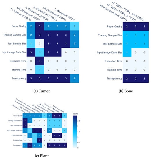
Figure 5. Comparison of machine learning image prediction models in three fields. Table (a) represents the evaluation of studies focusing on tumors, as cited in the following references [29,30,33,37,74,78,78]. Table (b) represents the evaluation of studies focusing on bone, as cited in the following references [43,66]. Table (c) represents the evaluation of studies focusing on plant, as cited in the following references [34,35,36,40,41,47,59].

We did not evaluate all 8 papers on blood vessels because these papers did not use ML technology. Criteria include whether the dataset size is specified, whether the image input size is specified, whether the algorithm details are specified, whether the execution time and training time are specified, etc., and the overall quality is determined in three levels. In the field of plants, seven papers were selected, and two of them were evaluated separately for each algorithm, for a total of nine data samples. S. Haung et al. [38] for a dataset consisting of 305 FIA plots, Landsat and LiDAR remote sensing data, and a combined auxiliary geospatial dataset; therefore, it is excluded from Figure 5c. Y. Wu and H. [31] were excluded from Figure 5a because they were predicted by 3D models from signal data. In several papers [33,37,74,76], leave-one-out cross-validation was used to improve learning efficiency on small datasets. Leave-one-out cross-validation involves extracting a single item from the dataset to be used as test data, while the remaining data is utilized as training data. The Ghosh et al. [53] paper is excluded from Figure 5b because it uses FE-based mechanoregulatory as input and outputs a prediction of major tissue growth on a macrotexture-optimized implant design after 120 days of healing time. Mandel et al. [32] use 695 samples from a dataset with 3D spine models to predict growth and therefore exclude them from Figure 5b.

Training sample size was evaluated as 1 for less than 1000, 2 for between 1000 and 2000, and 3 for greater than 2000. Test sample size was evaluated as 1 for less than 300, 2 for between 300 and 1000, and 3 for greater than 300. Input Image Data Size was evaluated in three levels depending on whether the resolution of the input image was greater than or equal to $256\times 256$. Although not a definite index, we set 1000 as a standard, which is a reasonable number of samples to be used empirically. The ratio of training data to training data is often set at 7:3, so 300, one-third of 1000, was used as the standard. Execution Time was evaluated based on the following criteria: 1 for less than 3 s, 2 for less than 7 s, and 3 for more than 7 s. Transparency was evaluated based on whether implementation details such as used software and framework, hardware stracture, and machine learning settings (the number of epochs, batch size, and layer size) were provided. We evaluated the Paper Quality by checking whether all the items related to the dataset were not blank, whether all the items related to time were not blank, and Transparency.

We have understood that growth prediction is feasible at various levels, such as the cellular level (Tumor cellularity), tissue and organismal level (Plant growth), tissue level (Vessel growth), and organismal level (Bone morphology) in Section 3.1 and Section 3.2. To predict changes in deer antler growth, such as the growth and replacement of antlers, we must consider which level of growth prediction would be most effective.

In the context of predicting changes in deer antler growth, particularly the growth and replacement of antlers, the organismal level (Bone morphology) appears to be the most relevant and effective level of growth prediction. This is because antler growth and replacement involve the development and remodeling of bone structures, which are directly related to the morphology of bones at the organismal level. Therefore, employing techniques used for predicting bone growth and development could potentially provide valuable insights into the changes in deer antler growth, including antler growth and replacement. These methods could be tailored to detect and quantify the changes in antler growth, taking into account the factors such as size, shape, and branching patterns. By integrating these approaches into a predictive model, it may be possible to accurately forecast changes in deer antler growth, thus enhancing our understanding of their growth patterns and contributing to better management and conservation strategies.

Through this SLR, we have deepened our consideration of the potential applicability of GANs for predicting changes in deer antler, such as antler growth and replacement. It should be noted here that this study is not based on cytology to predict growth but is rooted in the CV field, where analysis is performed from images captured by an RGB camera. The composition of deer antlers is divided into layers such as trabecular bone, cortical bone, and mesenchyme. While incorporating the growth characteristics of these compositions into a growth prediction model as physical equations is a possible future direction, it may be insufficient to account for the complex factors affecting bone growth in the wild, such as collisions, injuries, habitat, and food intake. In this regard, machine learning techniques that predict growth stages from images may be more effective in handling these hard cases, as they can learn to recognize and adapt to a wide range of real-world conditions and variations.

GANs, which learns from real-world hard data, has been successfully employed for growth prediction at the cellular level (Tumor cellularity) [33,37] and Tissue and organismal level (Plant growth) [47]. Given this success, it is worth considering the potential applicability of GANs for predicting changes in deer antler, such as antler growth and replacement. In the context of growth prediction, we conclude that GANs has potential to generate synthetic images representing different growth stages, making them a potential candidate for predicting changes in deer antler.

To assess the applicability of GANs for predicting changes in deer antler growth, several factors should be considered:

(a) Data availability: A large dataset of deer images at different growth stages, particularly focusing on antler development, is required for training the GANs. This dataset should include a diverse range of images that capture variations in antler size, shape, and branching patterns, as well as other relevant factors that may influence antler growth. Labeling the antler growth process in stages based on the number of branches and the date of antler growth makes it easy to adapt stage prediction combined with STN, as in the case of [35,59] et al. First, we will record the individual identification of deer by photographing deer kept in zoos and research facilities. Once the model is trained using these labeled images, we will then apply the learned knowledge to predict antler growth in wild deer populations.

(b) Model adaptation: The GANs architecture and training process should be adapted to the specific task of predicting changes in deer antler. This may involve fine-tuning the model architecture, loss functions, and optimization strategies to ensure that the generated images accurately represent the growth and replacement of antlers. We have not fully elaborated on the details of this process, and it will be the biggest challenge in future research.

(c) Evaluation metrics: Establishing appropriate evaluation metrics is crucial for assessing the performance of the GANs in predicting deer antler changes. These metrics should quantify the similarity between the generated images and the ground truth, taking into account factors such as antler shape, size, and branching patterns. In particular, it is important to comprehensively quantify the size and spacing of branches and the number of branches from size-normalized images, as described below for the pattern of bone branching. This is a reasonable idea since in some papers, the loss function is composed of a composite of indices. For example, in plants, the loss function for color and shape is defined and composited to obtain the final loss function [36]. It is easy to combine the loss functions based on the number of branches, size, color, and other indicators and define a new loss function; however, it is effective according to papers selected by this SLR.

In conclusion, while we conclude that GANs has potential in growth prediction tasks at the Cellular and Tissue and organismal levels, further research and experimentation are needed to determine their applicability for predicting changes in deer antler. By considering the factors mentioned above and adapting the GANs accordingly, it may be possible to develop a successful model for predicting changes in deer antler, including antler growth and replacement.

In addition to GAN-based methods, we also considered the prediction method extracting landmarks from bone images as in the paper by Mahsa Tajdari et al [66]. By specifying the corner points of each vertebra in the 2D frontal (AP) and lateral (LAT) X-ray images, Landmarks are detected with a semiautomatic method. The paper also extracts landmarks from the X-ray images to track non-uniform bone growth. Landmarks are selected for each vertebra, with four corners corresponding to the top and bottom of the growth plate, to obtain a good representation of the bone growth area. They constructed neural networks to predict the growth of cervical spine curvature, using landmark coordinates, global angles representing the overall spine curvature, and patient age as input data.

The above method cannot be directly applied to landmark extraction for deer antlers. However, it may be possible to establish a landmark representation of the mesenchyme and branches of deer antlers. In that case, we could use a similar neural network that takes landmarks, antler branches, their angles, their total angles, and age as inputs to predict antler shape. Because the method applied in [66] and our method share a similarity in that growth prediction which can be determined by landmarks and angles. Since the method [66] involves manually adjusting automatically generated landmarks at the final stage, manual landmark setting is worth considering in the early stages of research on antler growth prediction. However, antler growth prediction involves a large amount of image data, and it is not practical to manually set landmarks from all the image data. Therefore, we have to devise a (semi-)automatic landmark generation technique.

4.3. Implications for Future Research

As shown in Figure 4, there was a significant increase in DL in 2019 and 2020. We did not find many changes in the field of non-ML from 2017 to 2022. There were 26 publications related to non-ML studies, whereas only 21 were related to ML. This indicates that non-ML publications have dominated the ML publications in terms of growth prediction. There was no increment in ML publications between 2017 and 2018, where only a couple of publications were noted. However, we found a change in this trend after 2019 only. It was doubled in 2019 and sharply increased in 2020 and 2021, resulting in six publications in total in 2021.

Holes and scars on plants are either filled in or remain intact as the plant grows. Considering wounds as geometric features, it is reasonable to use STN, which can make predictions while preserving geometric features [35,59]. Although the examples of STN [35] are limited to datasets taken indoors from above, it is rather suitable for predicting environments where leaves are easily scratched, such as outdoors. Conversely, for the prediction of animal antlers, the entire image’s affine transformation is unsuitable for cases such as adult deer, whose physical characteristics do not change significantly except for the antlers. A possible application using partial STN would be to predict the growth of a specific part of the image (e.g., the growth of antlers at the end of a branch).

A study by Drees et al. [47] demonstrated the suitability of an unsupervised learning-based GAN technique for generating realistic images of future plant growth stages. In contrast, the STN study presented in this paper is classified as supervised machine learning, as it relies on pregrowth and actual postgrowth images. Since tracking the sequential growth of wild animals in images is challenging, especially considering our goal of individual animal identification, the paper’s findings on growth prediction by unsupervised learning pave the way for future research.

To improve the accuracy of plant growth prediction, Kim et al. [35] proposed a novel loss function for combining STN loss with RGB and shape loss. Meanwhile, other studies have introduced loss functions that minimize the geodesic distance between the sample and the regressed curve and metrics produced from simple distance spaces [32]. As complex geometry data become more prevalent, the adaptation of machine learning models to handle such data and the derivation of complex losses by combining existing ones will continue to evolve.

There are models that can make predictions based on data types other than images, such as signal or land data, and there are also models that can output 3D images as well as just 2D images [31,38]. Research on sensor fusion or image fusion, which involves obtaining images from various data sources, is increasing every year [90], and we can expect models that can make predictions using diverse data sources to continue developing.

5. Conclusions and Future Directions

In this study, we conducted a comprehensive SLR based on PRISMA guidelines for 47 articles related to growth predictions ranging from 2017 to 2022. Our objective of this study was to find out the research trend directly related to growth prediction techniques and algorithms. Our survey followed a systematic step prescribed by PRISMA guideline so that our conclusion is valid and reliable for future research. In this SLR, we extracted more than 526 articles in total from four electronic databases (i.e., IEEE Xplore, ACM Digital Library, Science Direct, and Web of Science) by using the search string introduced in Table 3. We found a few duplicates initially and thus excluded them from our SLR, while 438 articles were excluded based on title and abstract criteria. Articles having segmentation in their keywords and titles were also excluded, as we wanted to focus on growth prediction rather than segmentation. Additionally, articles that included the words: “crack”, “fatigue”, “urban”, “crystal”, and words related to metal were also removed. We set the inclusion and exclusion criteria to ensure that our conclusion is reliable. After these exclusions, the full texts of 88 studies were comprehensively analyzed and divided into machine-learning and non-machine learning models, with a focus on the machine learning models that appeared most frequently.

ML has made considerable progress in various fields, including zoology, agriculture, and medical science. We argue that while current growth prediction algorithms using image processing are primarily applied in the medical field. However, we noted that the challenge is still pertained to the field of individual animal recognition. The efficacy and reliability of ML-based individual recognition techniques can be improved by incorporating a variety of image types and employing MT. On the basis of this SLR, we concluded that it is possible to forecast growth not only by GAN but also by various other methods and to apply them to MT. This could lead to more reliable and effective results, especially considering changes in physical characteristics.

In conclusion, this SLR served as a showcase for scholars who wish to investigate the field of growth prediction using ML technologies. Our results highlighted the studies on the growth predictions particularly focusing on the organs of horns, tails, and other organs of wild animals. This study revealed a sizable vacuum in the literature on these particular characteristics and emphasized the potential of new research directions in this area. Researchers can better grasp these particular animal features’ genesis and evolution by digging deeper into their growth patterns. Furthermore, this study may shed light on the variables that affect the conservation efforts of wild animals, which could significantly impact conservation strategy.

We believe that this SLR makes a significant contribution to the field of growth prediction research, and we hope that it will encourage others to caliber their research in this emerging topic. Additionally, the results of this SLR serve as a significant starting point for the creation of novel growth prediction techniques and algorithms, opening the door to more precise and trustworthy forecasts in various fields, including but not limited to medicine, agriculture, and wildlife conservation. Overall, this SLR paves the way for growth prediction research, and we are forward to report additional findings in our following articles.

References

- Kumar, S.; Singh, S.K.; Singh, A.K. Muzzle point pattern based techniques for individual cattle identification. IET Image Process. 2017, 11, 805–814. [Google Scholar] [CrossRef]
- Awad, A.I.; Hassaballah, M. Bag-of-visual-words for cattle identification from muzzle print images. Appl. Sci. 2019, 9, 4914. [Google Scholar] [CrossRef]
- Kumar, S.; Pandey, A.; Satwik, K.S.R.; Kumar, S.; Singh, S.K.; Singh, A.K.; Mohan, A. Deep learning framework for recognition of cattle using muzzle point image pattern. Measurement 2018, 116, 1–17. [Google Scholar] [CrossRef]
- Bello, R.W.; Talib, A.Z.H.; Mohamed, A.S.A.B. Deep belief network approach for recognition of cow using cow nose image pattern. Walailak J. Sci. Technol. (WJST) 2021, 18, 8914–8984. [Google Scholar] [CrossRef]
- Mimura, S.; Itoh, K.; Kobayashi, T.; Takigawa, T.; Tajima, A.; Sawamura, A.; Otsu, N. The Cow Gait Recognition Using CHLAC. In Proceedings of the 2008 Bio-Inspired, Learning and Intelligent Systems for Security, Edinburgh, UK, 4–6 August 2008; pp. 56–57. [Google Scholar] [CrossRef]
- Okura, F.; Ikuma, S.; Makihara, Y.; Muramatsu, D.; Nakada, K.; Yagi, Y. RGB-D video-based individual identification of dairy cows using gait and texture analyses. Comput. Electron. Agric. 2019, 165, 104944. [Google Scholar] [CrossRef]
- Sharma, S.; Jhala, Y.; Sawarkar, V.B. Identification of individual tigers (Panthera tigris) from their pugmarks. J. Zool. 2005, 267, 9–18. [Google Scholar] [CrossRef]
- Roughan, J.V.; Sevenoaks, T. Welfare and scientific considerations of tattooing and ear tagging for mouse identification. J. Am. Assoc. Lab. Anim. Sci. 2019, 58, 142–153. [Google Scholar] [CrossRef]
- Zin, T.T.; Pwint, M.Z.; Seint, P.T.; Thant, S.; Misawa, S.; Sumi, K.; Yoshida, K. Automatic Cow Location Tracking System Using Ear Tag Visual Analysis. Sensors 2020, 20, 3564. [Google Scholar] [CrossRef]
- Pretto, A.; Savio, G.; Gottardo, F.; Uccheddu, F.; Concheri, G. A novel low-cost visual ear tag based identification system for precision beef cattle livestock farming. Inf. Process. Agric. 2022. [Google Scholar] [CrossRef]
- Harie, Y.; Neupane, S.B.; Gautam, B.P.; Norio, S. Augmented Triplet Network for Individual Organism and Unique Object Classification for Reliable Monitoring of Ezoshika Deer. In Proceedings of the IEEE 2021 Ninth International Symposium on Computing and Networking Workshops (CANDARW), Matsue, Japan, 23–26 November 2021; pp. 197–200. [Google Scholar]
- Clapham, M.; Miller, E.; Nguyen, M.; Darimont, C.T. Automated facial recognition for wildlife that lack unique markings: A deep learning approach for brown bears. Ecol. Evol. 2020, 10, 12883–12892. [Google Scholar] [CrossRef] [PubMed]
- Zhang, M.; Zhang, Y.; Zhang, L.; Liu, C.; Khurshid, S. DeepRoad: GAN-Based Metamorphic Testing and Input Validation Framework for Autonomous Driving Systems. In Proceedings of the 33rd ACM/IEEE International Conference on Automated Software Engineering, Montpellier, France, 3–7 September 2018; pp. 132–142. [Google Scholar] [CrossRef]
- Chen, T.Y.; Kuo, F.C.; Liu, H.; Poon, P.L.; Towey, D.; Tse, T.H.; Zhou, Z.Q. Metamorphic testing: A review of challenges and opportunities. ACM Comput. Surv. (CSUR) 2018, 51, 1–27. [Google Scholar] [CrossRef]
- Jing-jie, J.; Luo, X.U.; Ning, L.I. Method of Metamorphic Testing for Image Recognition System Based on GAN. Comput. Mod. 2021, 0, 24–29. [Google Scholar]
- Park, H.; Waseem, T.; Teo, W.Q.; Low, Y.H.; Lim, M.K.; Chong, C.Y. Robustness Evaluation of Stacked Generative Adversarial Networks using Metamorphic Testing. In Proceedings of the 2021 IEEE/ACM 6th International Workshop on Metamorphic Testing (MET), Madrid, Spain, 2 June 2021; pp. 1–8. [Google Scholar]
- Pan, Y.; Ao, H.; Fan, Y. Metamorphic Testing for Autonomous Driving Systems in Fog based on Quantitative Measurement. In Proceedings of the 2021 IEEE 21st International Conference on Software Quality, Reliability and Security Companion (QRS-C), Hainan, China, 6–10 December 2021; pp. 30–37. [Google Scholar] [CrossRef]
- Browning, E.; Bolton, M.; Owen, E.; Shoji, A.; Guilford, T.; Freeman, R. Predicting animal behaviour using deep learning: GPS data alone accurately predict diving in seabirds. Methods Ecol. Evol. 2018, 9, 681–692. [Google Scholar] [CrossRef]
- Hossain, M.E.; Kabir, M.A.; Zheng, L.; Swain, D.L.; McGrath, S.; Medway, J. A systematic review of machine learning techniques for cattle identification: Datasets, methods and future directions. Artif. Intell. Agric. 2022, 6, 138–155. [Google Scholar] [CrossRef]
- Kumar, S.; Singh, S.K. Cattle recognition: A new frontier in visual animal biometrics research. Proc. Natl. Acad. Sci. India Sect. A Phys. Sci. 2020, 90, 689–708. [Google Scholar] [CrossRef]
- Vidal, M.; Wolf, N.; Rosenberg, B.; Harris, B.P.; Mathis, A. Perspectives on individual animal identification from biology and computer vision. Integr. Comp. Biol. 2021, 61, 900–916. [Google Scholar] [CrossRef]
- Van Klompenburg, T.; Kassahun, A.; Catal, C. Crop yield prediction using machine learning: A systematic literature review. Comput. Electron. Agric. 2020, 177, 105709. [Google Scholar] [CrossRef]
- Tavse, S.; Varadarajan, V.; Bachute, M.; Gite, S.; Kotecha, K. A Systematic Literature Review on Applications of GAN-Synthesized Images for Brain MRI. Future Internet 2022, 14, 351. [Google Scholar] [CrossRef]
- Sargun, K.; Mohan, S. Modeling the crop growth—A review. Mausam 2020, 71, 103–114. [Google Scholar] [CrossRef]
- Muruganantham, P.; Wibowo, S.; Grandhi, S.; Samrat, N.H.; Islam, N. A Systematic Literature Review on Crop Yield Prediction with Deep Learning and Remote Sensing. Remote Sens. 2022, 14, 1990. [Google Scholar] [CrossRef]
- Page, M.J.; McKenzie, J.E.; Bossuyt, P.M.; Boutron, I.; Hoffmann, T.C.; Mulrow, C.D.; Shamseer, L.; Tetzlaff, J.M.; Akl, E.A.; Brennan, S.E.; et al. The PRISMA 2020 statement: An updated guideline for reporting systematic reviews. Int. J. Surg. 2021, 88, 105906. [Google Scholar] [CrossRef] [PubMed]
- Kahla, R.B.; Barkaoui, A. Chapter 5—Bone and bone remodeling finite element modeling. In Bone Remodeling Process; Kahla, R.B., Barkaoui, A., Eds.; Academic Press: Cambridge, MA, USA, 2021; pp. 165–206. [Google Scholar] [CrossRef]
- Uchiyama, H.; Sakurai, S.; Mishima, M.; Arita, D.; Okayasu, T.; Shimada, A.; Taniguchi, R.I. An Easy-to-Setup 3D Phenotyping Platform for KOMATSUNA Dataset. In Proceedings of the 2017 IEEE International Conference on Computer Vision Workshops (ICCVW), Venice, Italy, 22–29 October 2017; pp. 2038–2045. [Google Scholar] [CrossRef]
- Wang, H.; Xiao, N.; Zhang, J.; Yang, W.; Ma, Y.; Suo, Y.; Zhao, J.; Qiang, Y.; Lian, J.; Yang, Q. Static–Dynamic coordinated Transformer for Tumor Longitudinal Growth Prediction. Comput. Biol. Med. 2022, 148, 105922. [Google Scholar] [CrossRef] [PubMed]
- Zhang, L.; Lu, L.; Wang, X.; Zhu, R.; Bagheri, M.; Summers, R.; Yao, J. Spatio-Temporal Convolutional LSTMs for Tumor Growth Prediction by Learning 4D Longitudinal Patient Data. IEEE Trans. Med. Imaging 2020, 39, 1114–1126. [Google Scholar] [CrossRef]
- Wu, Y.; Zhu, H. Investigation of Long Short -Term Memory Based Ultrawide Band Microwave Breast Tumor Size Prediction. In Proceedings of the 2019 12th International Congress on Image and Signal Processing, BioMedical Engineering and Informatics (CISP-BMEI), Suzhou, China, 19–21 October 2019; pp. 1–6. [Google Scholar] [CrossRef]
- Mandel, W.; Oulbacha, R.; Roy-Beaudry, M.; Parent, S.; Kadoury, S. Image-Guided Tethering Spine Surgery With Outcome Prediction Using Spatio-Temporal Dynamic Networks. IEEE Trans. Med. Imaging 2021, 40, 491–502. [Google Scholar] [CrossRef] [PubMed]
- Elazab, A.; Wang, C.; Gardezi, S.J.S.; Bai, H.; Wang, T.; Lei, B.; Chang, C. Glioma Growth Prediction via Generative Adversarial Learning from Multi-Time Points Magnetic Resonance Images. In Proceedings of the 2020 42nd Annual International Conference of the IEEE Engineering in Medicine & Biology Society (EMBC), Montreal, QC, Canada, 20–24 July 2020; pp. 1750–1753. [Google Scholar] [CrossRef]
- Meng, Y.; Xu, M.; Yoon, S.; Jeong, Y.; Park, D. Flexible and high quality plant growth prediction with limited data. Front. Plant Sci. 2022, 13, 989304. [Google Scholar] [CrossRef]
- Kim, T.; Lee, S.H.; Kim, J.O. A Novel Shape Based Plant Growth Prediction Algorithm Using Deep Learning and Spatial Transformation. IEEE Access 2022, 10, 37731–37742. [Google Scholar] [CrossRef]
- Jung, J.; Lee, S.; Kim, T.; Oh, M.; Kim, J. Shape Based Deep Estimation of Future Plant Images. IEEE Access 2022, 10, 4763–4776. [Google Scholar] [CrossRef]
- Elazab, A.; Wang, C.; Gardezi, S.; Bai, H.; Hu, Q.; Wang, T.; Chang, C.; Lei, B. GP-GAN: Brain tumor growth prediction using stacked 3D generative adversarial networks from longitudinal MR Images. Neural Netw. 2020, 132, 321–332. [Google Scholar] [CrossRef]
- Huang, S.; Ramirez, C.; McElhaney, M.; Evans, K. F3: Simulating spatiotemporal forest change from field inventory, remote sensing, growth modeling, and management actions. For. Ecol. Manag. 2018, 415–416, 26–37. [Google Scholar] [CrossRef]
- Huang, C.J.; Lee, Y.J.; Wei, A.C. Cell Cycle Phase Classification from Deep Learning-Predicted Images of Cell Organelles. In Proceedings of the 2022 IEEE 22nd International Conference on Bioinformatics and Bioengineering (BIBE), Taichung, Taiwan, 7–9 November 2022; pp. 199–203. [Google Scholar] [CrossRef]
- Yi, W.; Dai, S.; Jiang, Y.; Yuan, C.; Yang, L. Computer-aided Visual Modeling of Rice Leaf Growth Based on Machine Learning. In Proceedings of the 2020 XXIII International Conference on Soft Computing and Measurements (SCM), Saint Petersburg, Russia, 27–29 May 2020; pp. 226–229. [Google Scholar] [CrossRef]
- Nesteruk, S.; Shadrin, D.; Kovalenko, V.; Rodríguez-Sánchez, A.; Somov, A. Plant Growth Prediction through Intelligent Embedded Sensing. In Proceedings of the 2020 IEEE 29th International Symposium on Industrial Electronics (ISIE), Delft, The Netherlands, 17–19 June 2020; pp. 411–416. [Google Scholar] [CrossRef]
- Chang, Y.H.; Abe, K.; Yokota, H.; Sudo, K.; Nakamura, Y.; Chu, S.L.; Hsu, C.Y.; Tsai, M.D. Human Induced Pluripotent Stem Cell Reprogramming Prediction in Microscopy Images using LSTM based RNN. In Proceedings of the 2019 41st Annual International Conference of the IEEE Engineering in Medicine and Biology Society (EMBC), Berlin, Germany, 23–27 July 2019; pp. 2416–2419. [Google Scholar] [CrossRef]
- Niño-Sandoval, T.C.; Pérez, S.V.G.; González, F.A.; Jaque, R.A.; Infante-Contreras, C. Use of automated learning techniques for predicting mandibular morphology in skeletal class I, II and III. Forensic Sci. Int. 2017, 281, 187.e1–187.e7. [Google Scholar] [CrossRef]
- Niño-Sandoval, T.C.; Perez, S.V.G.; Gonzalez, F.A.; Jaque, R.A.; Infante-Contreras, C. An automatic method for skeletal patterns classification using craniomaxillary variables on a Colombian population. Forensic Sci. Int. 2016, 261, 159.e1–159.e6. [Google Scholar] [CrossRef]
- Jarrett, A.; Hormuth, D.; Adhikarla, V.; Sahoo, P.; Abler, D.; Tumyan, L.; Schmolze, D.; Mortimer, J.; Rockne, R.; Yankeelov, T. Towards integration of Cu-64-DOTA-trastuzumab PET-CT and MRI with mathematical modeling to predict response to neoadjuvant therapy in HER2+breast cancer. Sci. Rep. 2020, 10, 20518. [Google Scholar] [CrossRef] [PubMed]
- Meng, Q.; Zuo, C.; Shi, F.; Zhu, W.; Xiang, D.; Chen, H.; Chen, X. Three-dimensional choroid neovascularization growth prediction from longitudinal retinal OCT images based on a hybrid model. Pattern Recognit. Lett. 2021, 146, 108–114. [Google Scholar] [CrossRef]
- Drees, L.; Junker-Frohn, L.V.; Kierdorf, J.; Roscher, R. Temporal prediction and evaluation of Brassica growth in the field using conditional generative adversarial networks. Comput. Electron. Agric. 2021, 190, 106415. [Google Scholar] [CrossRef]
- Isola, P.; Zhu, J.Y.; Zhou, T.; Efros, A.A. Image-to-image translation with conditional adversarial networks. In Proceedings of the IEEE Conference on Computer Vision and Pattern Recognition, Honolulu, HI, USA, 21–26 July 2017; pp. 1125–1134. [Google Scholar]
- Bernard, O.; Bosch, J.G.; Heyde, B.; Alessandrini, M.; Barbosa, D.; Camarasu-Pop, S.; Cervenansky, F.; Valette, S.; Mirea, O.; Bernier, M.; et al. Standardized evaluation system for left ventricular segmentation algorithms in 3D echocardiography. IEEE Trans. Med. Imaging 2015, 35, 967–977. [Google Scholar] [CrossRef]
- Khmag, A.; Al Haddad, S.A.R.; Ramlee, R.A.; Kamarudin, N.; Malallah, F.L. Natural image noise removal using nonlocal means and hidden Markov models in transform domain. Vis. Comput. 2018, 34, 1661–1675. [Google Scholar] [CrossRef]
- Jarrett, A.; Kazerouni, A.; Wu, C.; Virostko, J.; Sorace, A.; DiCarlo, J.; Hormuth, D.; Ekrut, D.; Patt, D.; Goodgame, B.; et al. Quantitative magnetic resonance imaging and tumor forecasting of breast cancer patients in the community setting. Nat. Protoc. 2021, 16, 5309–5338. [Google Scholar] [CrossRef]
- Chengyue, W. Available online: https://github.com/ChengyueWu/Quantitative-MRI-of-breast-cancer-patients-to-forecast-response-to-therapy (accessed on 22 February 2023).
- Ghosh, R.; Chanda, S.; Chakraborty, D. Qualitative predictions of bone growth over optimally designed macro-textured implant surfaces obtained using NN-GA based machine learning framework. Med. Eng. Phys. 2021, 95, 64–75. [Google Scholar] [CrossRef]
- Pleouras, D.S.; Sakellarios, A.I.; Loukas, V.S.; Kyriakidis, S.; Fotiadis, D.I. Prediction of the development of coronary atherosclerotic plaques using computational modeling in 3D reconstructed coronary arteries. In Proceedings of the 2020 42nd Annual International Conference of the IEEE Engineering in Medicine & Biology Society (EMBC), Montreal, QC, Canada, 20–24 July 2020; pp. 2808–2811. [Google Scholar] [CrossRef]
- Kigka, V.I.; Rigas, G.; Sakellarios, A.; Siogkas, P.; Andrikos, I.O.; Exarchos, T.P.; Loggitsi, D.; Anagnostopoulos, C.D.; Michalis, L.K.; Neglia, D.; et al. 3D reconstruction of coronary arteries and atherosclerotic plaques based on computed tomography angiography images. Biomed. Signal Process. Control 2018, 40, 286–294. [Google Scholar] [CrossRef]
- Kigka, V.I.; Sakellarios, A.; Kyriakidis, S.; Rigas, G.; Athanasiou, L.; Siogkas, P.; Tsompou, P.; Loggitsi, D.; Benz, D.C.; Buechel, R.; et al. A three-dimensional quantification of calcified and non-calcified plaques in coronary arteries based on computed tomography coronary angiography images: Comparison with expert’s annotations and virtual histology intravascular ultrasound. Comput. Biol. Med. 2019, 113, 103409. [Google Scholar] [CrossRef]
- Sakellarios, A.I.; Räber, L.; Bourantas, C.V.; Exarchos, T.P.; Athanasiou, L.S.; Pelosi, G.; Koskinas, K.C.; Parodi, O.; Naka, K.K.; Michalis, L.K.; et al. Prediction of Atherosclerotic Plaque Development in an In Vivo Coronary Arterial Segment Based on a Multilevel Modeling Approach. IEEE Trans. Biomed. Eng. 2017, 64, 1721–1730. [Google Scholar] [CrossRef] [PubMed]
- Do, H.N.; Ijaz, A.; Gharahi, H.; Zambrano, B.; Choi, J.; Lee, W.; Baek, S. Prediction of Abdominal Aortic Aneurysm Growth Using Dynamical Gaussian Process Implicit Surface. IEEE Trans. Biomed. Eng. 2019, 66, 609–622. [Google Scholar] [CrossRef] [PubMed]
- Kim, T.H.; Lee, S.H.; Oh, M.M.; Kim, J.O. Plant Growth Prediction Based on Hierarchical Auto-encoder. In Proceedings of the 2022 International Conference on Electronics, Information, and Communication (ICEIC), Jeju, Republic of Korea, 6–9 February 2022; pp. 1–3. [Google Scholar] [CrossRef]
- Zhang, L.; Jiang, Z.; Choi, J.; Lim, C.Y.; Maiti, T.; Baek, S. Patient-Specific Prediction of Abdominal Aortic Aneurysm Expansion Using Bayesian Calibration. IEEE J. Biomed. Health Inform. 2019, 23, 2537–2550. [Google Scholar] [CrossRef]
- Wong, K.; Summers, R.; Kebebew, E.; Yao, J. Pancreatic Tumor Growth Prediction With Elastic-Growth Decomposition, Image-Derived Motion, and FDM-FEM Coupling. IEEE Trans. Med. Imaging 2017, 36, 111–123. [Google Scholar] [CrossRef]
- Alonso, M.G.; Bertolino, G.; Yawny, A. Mechanobiological based long bone growth model for the design of limb deformities correction devices. J. Biomech. 2020, 109, 109905. [Google Scholar] [CrossRef] [PubMed]
- Jiang, Z.; Choi, J.; Baek, S. Machine learning approaches to surrogate multifidelity Growth and Remodeling models for efficient abdominal aortic aneurysmal applications. Comput. Biol. Med. 2021, 133, 104394. [Google Scholar] [CrossRef]
- Rekik, I.; Li, G.; Yap, P.T.; Chen, G.; Lin, W.; Shen, D. Joint prediction of longitudinal development of cortical surfaces and white matter fibers from neonatal MRI. NeuroImage 2017, 152, 411–424. [Google Scholar] [CrossRef]
- Fouad, H.; Hassanein, A.S.; Soliman, A.M.; Al-Feel, H. Internet of Medical Things (IoMT) Assisted Vertebral Tumor Prediction Using Heuristic Hock Transformation Based Gautschi Model–A Numerical Approach. IEEE Access 2020, 8, 17299–17309. [Google Scholar] [CrossRef]
- Tajdari, M.; Pawar, A.; Li, H.; Tajdari, F.; Maqsood, A.; Cleary, E.; Saha, S.; Zhang, Y.J.; Sarwark, J.F.; Liu, W.K. Image-based modelling for Adolescent Idiopathic Scoliosis: Mechanistic machine learning analysis and prediction. Comput. Methods Appl. Mech. Eng. 2021, 374, 113590. [Google Scholar] [CrossRef]
- Scheufele, K.; Subramanian, S.; Biros, G. Fully Automatic Calibration of Tumor-Growth Models Using a Single mpMRI Scan. IEEE Trans. Med. Imaging 2021, 40, 193–204. [Google Scholar] [CrossRef]
- Moon, J.; Kim, M.; Hwang, H.; Cho, S.; Donatelli, R.; Lee, S. Evaluation of an individualized facial growth prediction model based on the multivariate partial least squares method. Angle Orthod. 2022, 92, 705–713. [Google Scholar] [CrossRef]
- Matthews, H.; Penington, A.; Clement, J.; Kilpatrick, N.; Fan, Y.; Claes, P. Estimating age and synthesising growth in children and adolescents using 3D facial prototypes. Forensic Sci. Int. 2018, 286, 61–69. [Google Scholar] [CrossRef] [PubMed]
- Kainz, H.; Killen, B.A.; Campenhout, A.V.; Desloovere, K.; Aznar, J.M.G.; Shefelbine, S.; Jonkers, I. ESB Clinical Biomechanics Award 2020: Pelvis and hip movement strategies discriminate typical and pathological femoral growth – Insights gained from a multi-scale mechanobiological modelling framework. Clin. Biomech. 2021, 87, 105405. [Google Scholar] [CrossRef] [PubMed]
- Subramanian, S.; Ghafouri, A.; Scheufele, K.; Himthani, N.; Davatzikos, C.; Biros, G. Ensemble inversion for brain tumor growth models with mass effect. IEEE Trans. Med. Imaging 2022, 42, 982–995. [Google Scholar] [CrossRef] [PubMed]
- Subramanian, S. Available online: https://github.com/ShashankSubramanian/GLIA (accessed on 22 February 2023).
- Scheufele, K.; Mang, A.; Gholami, A.; Davatzikos, C.; Biros, G.; Mehl, M. Coupling brain-tumor biophysical models and diffeomorphic image registration. Comput. Methods Appl. Mech. Eng. 2019, 347, 533–567. [Google Scholar] [CrossRef] [PubMed]
- Zhang, L.; Lu, L.; Summers, R.; Kebebew, E.; Yao, J. Convolutional Invasion and Expansion Networks for Tumor Growth Prediction. IEEE Trans. Med. Imaging 2018, 37, 638–648. [Google Scholar] [CrossRef] [PubMed]
- Moult, E.M.; Shi, E.A. Comparing Accuracies of Length-Type Geographic Atrophy Growth Rate Metrics Using Atrophy-Front Growth Modeling. Ophthalmol. Sci. 2022, 2, 100156. [Google Scholar] [CrossRef]
- Elazab, A.; Anter, A.M.; Bai, H.; Hu, Q.; Hussain, Z.; Ni, D.; Wang, T.; Lei, B. An optimized generic cerebral tumor growth modeling framework by coupling biomechanical and diffusive models with treatment effects. Appl. Soft Comput. 2019, 80, 617–627. [Google Scholar] [CrossRef]
- Zhang, Y.; Zhang, X.; Ji, Z.; Niu, S.; Leng, T.; Rubin, D.L.; Yuan, S.; Chen, Q. An integrated time adaptive geographic atrophy prediction model for SD-OCT images. Med. Image Anal. 2021, 68, 101893. [Google Scholar] [CrossRef]
- Wang, L.; Wang, S.; Yu, H.; Zhu, Y.; Li, W.; Tian, J. A Quarter-split Domain-adaptive Network for EGFR Gene Mutation Prediction in Lung Cancer by Standardizing Heterogeneous CT image. In Proceedings of the 2021 43rd Annual International Conference of the IEEE Engineering in Medicine & Biology Society (EMBC), Online, 1–5 November 2021; pp. 3646–3649. [Google Scholar] [CrossRef]
- Bell, J.; Dee, H.M. Aberystwyth Leaf Evaluation Dataset; Zenodo: Honolulu, HI, USA, 2016. [Google Scholar] [CrossRef]
- Meyerowitz, E.M. Arabidopsis thaliana. Annu. Rev. Genet. 1987, 21, 93–111. [Google Scholar] [CrossRef]
- Malavazos, K.; Papadogiorgaki, M.; Malakonakis, P.; Papaefstathiou, I. A novel FPGA-based system for Tumor Growth Prediction. In Proceedings of the 2020 Design, Automation & Test in Europe Conference & Exhibition (DATE), Grenoble, France, 9–13 March 2020; pp. 252–257. [Google Scholar] [CrossRef]
- RIDER NEURO MRI—The Cancer Imaging Archive (TCIA) Public Access—Cancer Imaging Archive Wiki. Available online: https://wiki.cancerimagingarchive.net/display/Public/RIDER+NEURO+MRI (accessed on 22 February 2023).
- Dong, H.; Liu, M.; Qin, T.; Liang, L.; Ziganshin, B.; Ellauzi, H.; Zafar, M.; Jang, S.; Elefteriades, J.; Sun, W.; et al. A novel computational growth framework for biological tissues: Application to growth of aortic root aneurysm repaired by the V-shape surgery. J. Mech. Behav. Biomed. Mater. 2022, 127, 105081. [Google Scholar] [CrossRef] [PubMed]
- Rahman, M.; Feng, Y.; Yankeelov, T.; Oden, J. A fully coupled space-time multiscale modeling framework for predicting tumor growth. Comput. Methods Appl. Mech. Eng. 2017, 320, 261–286. [Google Scholar] [CrossRef] [PubMed]
- Roque, T.; Risser, L.; Kersemans, V.; Smart, S.; Allen, D.; Kinchesh, P.; Gilchrist, S.; Gomes, A.L.; Schnabel, J.A.; Chappell, M.A. A DCE-MRI Driven 3-D Reaction-Diffusion Model of Solid Tumor Growth. IEEE Trans. Med. Imaging 2018, 37, 724–732. [Google Scholar] [CrossRef] [PubMed]
- Pleouras, D.; Sakellarios, A.I.; Kyriakidis, S.; Kigka, V.; Siogkas, P.; Tsompou, P.; Tachos, N.; Georga, E.; Andrikos, I.; Rocchiccioli, S.; et al. A computational multi-level atherosclerotic plaque growth model for coronary arteries. In Proceedings of the 2019 41st Annual International Conference of the IEEE Engineering in Medicine and Biology Society (EMBC), Berlin, Germany, 23–27 July 2019; pp. 5010–5013. [Google Scholar] [CrossRef]
- Sudhakar, K.; Smail, B.; Reddy, T.S.; Shitharth, S.; Tripathi, D.R.; Fahlevi, M. Web User Profile Generation and Discovery Analysis using LSTM Architecture. In Proceedings of the 2022 2nd International Conference on Technological Advancements in Computational Sciences (ICTACS), Tashkent, Uzbekistan, 10–12 October 2022; pp. 371–375. [Google Scholar] [CrossRef]
- Banik, S.; Sharma, N.; Mangla, M.; Mohanty, S.N.; Shitharth, S. LSTM based decision support system for swing trading in stock market. Knowl. Based Syst. 2022, 239, 107994. [Google Scholar] [CrossRef]
- Ayub, S.; Kannan, R.J.; Shitharth, S.; Alsini, R.; Hasanin, T.; Sasidhar, C. LSTM-Based RNN Framework to Remove Motion Artifacts in Dynamic Multicontrast MR Images with Registration Model. Wirel. Commun. Mob. Comput. 2022, 2022, 5906877. [Google Scholar] [CrossRef]
- Liu, Y.; Wang, L.; Cheng, J.; Li, C.; Chen, X. Multi-focus image fusion: A survey of the state of the art. Inf. Fusion 2020, 64, 71–91. [Google Scholar] [CrossRef]
Disclaimer/Publisher’s Note: The statements, opinions and data contained in all publications are solely those of the individual author(s) and contributor(s) and not of MDPI and/or the editor(s). MDPI and/or the editor(s) disclaim responsibility for any injury to people or property resulting from any ideas, methods, instructions or products referred to in the content. |
© 2023 by the authors. Licensee MDPI, Basel, Switzerland. This article is an open access article distributed under the terms and conditions of the Creative Commons Attribution (CC BY) license (https://creativecommons.org/licenses/by/4.0/).