Fine-Tuning of Pre-Trained Deep Face Sketch Models Using Smart Switching Slime Mold Algorithm

Abstract

There are many pre-trained deep learning-based face recognition models developed in the literature, such as FaceNet, ArcFace, VGG-Face, and DeepFace. However, performing transfer learning of these models for handling face sketch recognition is not applicable due to the challenge of limited sketch datasets (single sketch per subject). One promising solution to mitigate this issue is by using optimization algorithms, which will perform a fine-tuning and fitting of these models for the face sketch problem. Specifically, this research introduces an enhanced optimizer that will evolve these models by performing automatic weightage/fine-tuning of the generated feature vector guided by the recognition accuracy of the training data. The following are the key contributions to this work: (i) this paper introduces a novel Smart Switching Slime Mold Algorithm (S²SMA), which has been improved by embedding several search operations and control rules; (ii) the proposed S²SMA aims to fine-tune the pre-trained deep learning models in order to improve the accuracy of the face sketch recognition problem; and (iii) the proposed S²SMA makes simultaneous fine-tuning of multiple pre-trained deep learning models toward further improving the recognition accuracy of the face sketch problem. The performance of the S²SMA has been evaluated on two face sketch databases, which are XM2VTS and CUFSF, and on CEC’s 2010 large-scale benchmark. In addition, the outcomes were compared to several variations of the SMA and related optimization techniques. The numerical results demonstrated that the improved optimizer obtained a higher level of fitness value as well as better face sketch recognition accuracy. The statistical data demonstrate that S²SMA significantly outperforms other optimization techniques with a rapid convergence curve.

1. Introduction

Face sketch recognition involves matching two face images from different modalities; one is a face drawing created by a professional artist based on a witness statement, and the other is the corresponding image from the agency’s department database. Some facial sketches are depicted for illustrative purposes, as given in Figure 1. Due to the partial and approximate nature of the eyewitness’s description, face sketches are less detailed than their corresponding photos. Due to the modality disparities between face photos and sketch images, classic homogeneous face recognition algorithms perform badly in face sketch recognition [1]. To overcome this challenge, soft computing models have been utilized. Existing methods for face sketch recognition are resolved in three ways, which are synthesis-based, projection-based, and optimization-based. In the first category, synthesis-based methods, also known as generative methods, are used to transform one of the modalities into the other (photo to sketch or vice versa) prior to matching [2,3,4,5,6,7,8,9,10,11]. Projection-based techniques utilize soft computing approaches [12,13,14,15,16,17] to reduce the differences between sketch and photo features projected in a different space. The final category, which is optimization-based, focuses on fine-tuning the parameters using optimization methods. In other words, the objective is to maximize the similarity between the sketch and its photo, maximizing the weights of their extracted features [1,18,19,20].

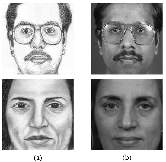
Figure 1. Sample of sketches (a) and corresponding photos (b).

Apart from that, deep learning approaches such as FaceNet [21], ArcFace [22], VGG-Face [23], and DeepFace [24] have recently achieved major advances in face recognition by learning latent embeddings from large amounts of face data. However, it is more difficult to use deep learning for face sketch recognition due to the lack of face sketch–photo data. This is due to the challenge of obtaining face sketch pictures where existing public datasets contain only a handful of face sketch–photo combinations, with one sketch per individual in most cases. Over-fitting and local minima arise from these limitations, making it hard for deep networks to learn adequate feature representations for face sketch recognition during training [25]. This study suggests adopting a recent optimization approach to solve this problem by performing fine-tuning of those pre-trained deep-face recognition models such as FaceNet, ArcFace, VGG-Face, and DeepFace.

Recently, several optimizers have been presented in the literature, such as Fitness Dependent Optimizer (FDO) [26], Donkey and Smuggler Optimizer (DSO) [27], Slime Mold Algorithm (SMA) [28], Black Widow Optimization Algorithm (BWO) [29], The Red Fox Optimization Algorithm (RFO) [30], Q-Learning Embedded Sine Cosine Algorithm (QLESCA) [31], and Reptile Search Algorithm (RSA) [32]. Among them, SMA received a lot of attention due to its smooth structure, few parameters, robustness, and implementation flexibility. However, when dealing with complicated and high-dimensional situations, SMA still has some limitations, such as its slow convergence and potential to slip into the local optima trap [33,34,35]. Additionally, the optimization algorithm for slime molds utilizes the best leader and two randomly pooled slime molds from the population, resulting in poor exploitation and exploration [36,37]. Thus, in order to fully optimize the performance of SMA and make it perfect for the face sketch recognition problem, we propose an enhanced variant named S²SMA. Accordingly, S²SMA will be applied to tackle the face sketch recognition problem.

In summary, this work presents S²SMA with embedded rules and search operations, namely the Arithmetic Optimization Algorithm (AOA) and the Levy Flight (LF). Moreover, S²SMA has been applied to tune the weights of deep-face models to make it work for the problem of face sketch recognition. Specifically, a total of four deep-face models were combined, and the proposed algorithm gives weights to each model to obtain the highest accuracy for face sketch recognition. The principal contributions to this paper are as follows:

• To propose an improved method for solving large-scale problems, which is called S²SMA. This work presents S²SMA with embedded rules and operations, namely AOA and LF. The AOA operation aims to solve the problem of SMA’s limited exploitation. Moreover, the LF mechanism has been integrated to improve SMA’s exploratory capability and aid in maintaining an appropriate balance between exploration and exploitation [38]. Furthermore, the proposed embedded smart switching rules allow for adaptive switching between search operations during execution.
• To formulate an optimized deep-face sketch recognition problem by fine-tuning the weights of deep features using S²SMA. As such, S²SMA tunes the weights of the outputs of the deep-face models to maximize the similarity between sketch–photo pairs. Here, S²SMA adjusts the weights of these models’ outputs to fit the face sketch recognition problem.
• To further enhance the deep-face sketch recognition by fine-tuning multiple deep models, four deep-face models specialized in facial recognition are used in this study: FaceNet [21], ArcFace [22], VGG-Face [23], and DeepFace [24]. These models are combined, and the proposed S²SMA gives weight to each model to obtain the highest accuracy for the face sketch recognition problem.

The remainder of this article is structured as follows. The following section presents a quick overview of the relevant research on face sketch recognition and SMA. Section 3 describes the SMA’s’ specifications and the details of the proposed work. The numerical experiment and statistical analysis are presented in Section 4. Finally, this paper is concluded in Section 5.

2. Related Work

As previously mentioned, face sketch recognition methods can be categorized into synthesis-based, projection-based, and optimization-based. This section highlights the studies that have followed the optimization methods. Many optimization approaches are used in the literature for face recognition, e.g., PSO-based [39,40,41,42,43], Firefly Optimization Algorithm-based [44], Harris Hawks Optimization-based [45], and Bald Eagle Search Optimization-based [46], which have been effectively applied to the problem of face recognition. However, only these studies focused on optimization-based methods for handling the problem of face sketch recognition. For example, the earliest study mentioned in this literature review is by Bhatt et al. [18], who proposed a weight optimization technique based on the Genetic Algorithm (GA) to determine the optimal weights for every facial patch. Their model was evaluated on sketch–digital picture pairs from the CUHK and IIIT-D databases. The results indicated that their approach could offer superior identification performance compared to existing algorithms. Later, Bhatt et al. (2012) combined the Genetic Algorithm (GA) and Simulated Annealing (SA) to address the issue of face sketch recognition [19]. GA-SA adjusted the weights of extracted features via a Local Binary Pattern (LBP). The experiments showed that the GA-SA method was better than other face recognition algorithms and two commercial systems. Moving to recent studies, Samma et al. (2019) introduced a hybrid optimization model that combined PSO and a local search strategy to perform localization and weighting of the facial sketch region [1]. They employed three distinct extraction strategies for texture features: Histogram of Gradient (HOG), Local Binary Pattern (LBP), and Gabor wavelet. Several datasets were used to assess their proposed hybrid model, such as LFW, AR, and CUHK. The results demonstrated that the hybrid model achieved 96% on AR, 87.68% on CUHK, and 50% on LFW. Statistically, the suggested approach outperforms PSO-based models and state-of-the-art optimization methods. In the most recent study, Samma et al. (2022) introduced a hybrid deep learning model for face sketch recognition that combined Particle Swarm Optimization (PSO) with the VGG-face deep learning network [20]. Their work incorporated PSO to determine the necessary VGG-facial filters and fine-tuned the weights of these selected filters for face sketch recognition. The outcomes showed PSO’s ability to improve model accuracy and reduce complexity.

Recent studies explored non-optimization-based methods for handling face sketch recognition. Ren et al. [47] presented an unsupervised CycleGAN-based model that converted face sketches into high-quality photos by incorporating a multi-scale feature extraction module and a CBAM module to improve feature extraction and reduce background interference. Rizkinia et al. [48] proposed a GAN-based method for generating color face photos from hand-drawn sketches with improved accuracy and reduced artifacts. The proposed method by Zhong et al. [49], called Unsupervised Self-Attention Lightweight photo-to-sketch synthesis with Feature Maps (USAL), added a self-attention module to a generative adversarial network and reduced the layers of the discriminator to improve efficiency and performance. Furthermore, C. Peng et al. [50] proposed an Intra-Domain Enhancement (IDE) method for face photo–sketch synthesis. The MLA-GAN model was designed to refine and extract features and enhance the resolution of the synthesized image, which outperformed the state-of-the-art face sketch synthesis methods on multiple public face sketch databases. In addition, Y. Peng et al. [51] introduced a Sketch-Guided Latent Diffusion Model (SGLDM) that used a Multi-Auto-Encoder (AE) to encode input sketches for denoising. The paper also proposed Stochastic Region Abstraction (SRA) as a data augmentation strategy to improve the model’s robustness in managing sketches with varying levels of abstraction. The SGLDM outperformed state-of-the-art methods and could synthesize high-quality face images with different expressions, facial accessories, and hairstyles. Earlier, Singh et al. [52] provided more information about digital image denoising based on a comprehensive overview of the backpropagation algorithm. However, these recent studies well demonstrated significant progress in the development of effective and efficient methods for handling face sketch recognition.

In the literature, the SMA has been applied to solve a wide variety of real-world problems, such as economic emission dispatch [53], image segmentation [54], and the estimation of solar photovoltaic cell parameters [55]. Researchers proposed several variations of the SMA to further enhance its performance in specific domains. Naik et al. [36] proposed a unique NSD-based multilevel thresholding strategy that employed the Leader Slime Mold Algorithm (LSMA). The LSMA outperformed the traditional SMA by using the three best candidates as a leader to guide the search. The study also applied the NSD-LSMA method for multilevel thresholding of Landsat images and showed that it outperformed state-of-the-art methods. In another study, Naik et al. [37] introduced an Adaptive Opposition Slime Mold Algorithm (AOSMA) for function optimization that adaptively decided whether to use opposition-based learning to enhance exploration and replaced one random search agent with the best one to maximize exploitation. The AOSMA outperformed other state-of-the-art optimization algorithms in qualitative and quantitative analyses. The algorithm was suggested to be useful for function optimization to solve real-world engineering problems. Concurrently, another study by Naik et al. [56] showed the development of a new Equilibrium Slime Mold Algorithm (ESMA) for multilevel thresholding of breast thermogram images based on minimizing the entropic dependencies among different classes in the image. The ESMA was evaluated and compared to other optimization algorithms and found to perform better. The study claimed that the proposed method might be useful for assisting medical practitioners in breast thermogram analysis. Chauhan et al. [57] proposed HAOASMA, a hybrid algorithm that combined AOA and SMA to address the limitations of SMA’s exploration and exploitation capabilities. They integrated lens opposition-based learning to increase population diversity and accelerate convergence. HAOASMA outperformed traditional SMA algorithms and is better for finding optimal global solutions. Recently, Altay [58] proposed the Chaotic SMA (CSMA) to improve the SMA method by applying ten different chaotic maps to generate chaotic values instead of random values. It was intended to speed up SMA’s global convergence and keep it from becoming trapped in its local solutions using chaotic maps. CSMA performed better in 62 benchmark functions and real-world engineering design challenges than other methods and standard SMA. Although very few studies have attempted to use different optimization techniques to solve the face sketch recognition problem, none have used SMA and its variants. Therefore, the current study aims to conduct further investigation on the effectiveness of the optimization algorithms to solve the face sketch recognition problem and to develop a new algorithm to deal with large-scale problems, including the face sketch recognition problem. In addition, the use of multiple pre-trained deep learning models and their simultaneous fine-tuning using S²SMA can be considered a novel approach to improve the accuracy of face sketch recognition.

3. Proposed SMA-Based Method

3.1. The Original Slime Mold Algorithm (SMA)

The SMA is a novel swarm intelligence optimization algorithm recently proposed by Li et al. [28], which simulates the foraging behavior of slime molds. The SMA consists of three phases: approaching, wrapping, and grabbing food.

3.1.1. Approaching Food

For a slime mold to approach food, the concentration of odor in the air is crucial. This contraction pattern while approaching food is defined by Equation (1):

$$\overrightarrow{X\left(t+1\right)}=\left\{\begin{array}{c}\overrightarrow{X_b\left(t\right)}+\overrightarrow{vb}·\left(\overrightarrow{W}·\overrightarrow{X_A\left(t\right)}-\overrightarrow{X_B\left(t\right)}\right), r_2<p\\ \overrightarrow{vc}·\overrightarrow{X\left(t\right)},r_2\ge p\end{array}\right.$$

(1)

where $\overrightarrow{vb}$ is a parameter with the interval [−a, a] and $\overrightarrow{vc}$ decreases from one to zero linearly. $\overrightarrow{X_b}$ indicates the individual position with the highest odor concentration currently discovered, $\overrightarrow{X}$ represents the current location of a slime mold, $\overrightarrow{X_A}$ and $\overrightarrow{X_B}$ represent two chosen randomly individuals from the $\mathrm{n}$ population, $t$ and $r_2$ represent the current number of iterations and a random value within [0, 1], respectively, and $\overrightarrow{W}$ denotes the weight of the slime mold. The parameter p is calculated as in Equation (2):

$$p=\mathit{tanh}\left|S\left(i\right)-DF\right|$$

(2)

where $\mathrm{i}\in 1,2,\dots ,\mathrm{n}$, $S\left(i\right)$ indicates the fitness of $\overrightarrow{\mathrm{X}}$ and $\mathrm{DF}$ represents the best fitness obtained throughout all iterations. The formula of $\overrightarrow{\mathrm{vb}}$ is shown in Equation (2), where $a$ is given in Equation (4):

$$\overrightarrow{vb}=\left[-a, a\right]$$

(3)

$$a=arctanh(-\left(\frac{t}{max\text{\_}t}\right)+1)$$

(4)

Here, $max\text{\_}t$ is the maximum number of iterations, the formula of $\overrightarrow{W}$ is listed in Equation (5), and it’s $SmellIndex$ is defined in Equation (6):

$$\overrightarrow{W\left(SmellIndex\left(i\right)\right)}=\left\{\begin{array}{c}1+r_3·\mathit{log}\left(\frac{bF-S\left(i\right)}{bF-wF}+1\right),condition \\ 1-r_3·\mathit{log}\left(\frac{bF-S\left(i\right)}{bF-wF}+1\right), others\end{array}\right.$$

(5)

$$SmellIndex=sort\left(S\right)$$

(6)

where $condition$ indicates that $S\left(i\right)$ ranks in the top fifty percent of the overall population, ${\mathrm{r}}_3$ represents a random value within [0, 1], the best fitness value obtained in the current iterative process is denoted by $bF$, the worst fitness value is denoted by $wF$, and $\mathrm{SmellIndex}$ represents the series of fitness values arranged in ascending order of fitness (ascends in the minimum value problem).

3.1.2. Wrapping Food

The mathematical formula for updating the location of the slime mold is given in Equation (7):

$$\overrightarrow{X^{\text{*}}\left(t+1\right)}=\left\{\begin{array}{cc}\hfill r_4·\left(UB-LB\right)+LB,r_1<z& \\ \hfill \overrightarrow{X_b\left(t\right)}+\overrightarrow{vb}·\left(W·\overrightarrow{X_A\left(t\right)}-\overrightarrow{X_B\left(t\right)}\right),r_2<p& and r_1\ge z \hfill \\ \hfill \overrightarrow{vc}·\overrightarrow{X\left(t\right)},r_2\ge p& and r_1\ge z \hfill \end{array}\right.$$

(7)

$r_1,{ \mathrm{r}}_2$, and ${\mathrm{r}}_4$ are random values in the interval [0, 1], where $LB$ and $UB$ represent the lower and upper search range bounds, respectively. The $p$ value represents the probability of a slime mold and $z$ is a parameter with a fixed value of 0.03.

Equation (7) has two switching parameters. $z$ is the first parameter that increases local exploration when individuals find less information near a targeted meal. This value may be an SMA characteristic; if slimes receive less knowledge for the global optimal, the algorithm chooses some slimes to abandon the current exploration and start over. On the other hand, $p$ is the second parameter that guides slimes to explore or exploit in each iteration. This value balances exploration and exploitation during iterations. The proper value could decrease the rate of slimes trapped in local optima.

3.1.3. Grabbling Food

$\overrightarrow{W}$, $\overrightarrow{vb}$, and $\overrightarrow{vc}$ are applied to represent the changes in slime mold venous width. $\overrightarrow{W}$ replicates the oscillating frequency of slime molds by analyzing the food’s quality to update the food’s speed, thus assisting slime molds in selecting the ideal food source. The values of $\overrightarrow{vb}$ and $\overrightarrow{vc}$ are oscillated randomly within a certain range. $\overrightarrow{vb}$ is within $\left[-a, a\right]$, while $\overrightarrow{vc}$ within [−1, 1]; additionally, as a result of the iterative process, they all converge on zero. In addition, the variation process of $\overrightarrow{vb}$ replicates whether the slime mold approaches or seeks out alternative food sources when a new food source is identified. The slime mold will always separate some organic matter to search for higher-quality food sources in other places, even if a superior food source has been discovered. This conduct increases the slime mold’s chances of locating higher-quality food and improves the optimal local problem. Additional information on the SMA can be found in the study of Li et al. [28].

3.2. Smart Switching Slime Mold Algorithm (S²SMA)

As explained in Equation (7), the SMA relies on this equation to update slime positions during the exploration and exploitation phases. Moreover, the SMA depends on z and p parameters to switch from exploration to exploitation and vice versa. However, the SMA still suffers from poor exploitative behavior, thus from slow convergence, and lacks potentially better solutions, which eventually require improvement. To overcome these shortcomings of the SMA, three modifications have been made to the original algorithm, which are summarized as follows:

• The first improvement, the SMA exploration phase, has been improved by incorporating LF into the original equation that updates the slime’s position in the wrap food phase in Equation (7).
• The second improvement, an embedded operation, was added from the AOA algorithm [59] to improve the exploitation phase further.
• The final improvement, a total of four embedded switching rules have been added to control switching between AOA, LF, and other SMA search operations.

3.2.1. The Proposed Embedded Levy Flight

The first part of the modification was to the original SMA by adding the Levy Flight to the SMA in Equation (7). LF is used to update the positions of the search agents and increase the search space [60], as well as to ensure the effective exploration position and avoid local convergence [61]. Moreover, LF maintains an appropriate balance between exploration and exploitation [62]. The expression is added to the SMA, and the following is how the embedded Levy Flight operation is added to the SMA equations, as given in Equation (8):

$$\overrightarrow{X}\left(t+1\right)=\overrightarrow{vc}\ast \overrightarrow{X}\left(t\right)+\overrightarrow{R}\times \overrightarrow{Lev{y}_{walk}}\left(dim\right)\times \left(\overrightarrow{X}\left(t\right)-\overrightarrow{X_b\left(t\right)}\right)$$

(8)

where $dim$ is the problem’s dimension, $\overrightarrow{R}$ is a random vector of size 1 × dim, and $Lev{y}_{walk}$ is the Levy Flight function, which is computed in Equation (9):

$$Lev{y}_{walk}\left(x\right)=0.01\times \frac{s\times \sigma }{{\left|p\right|}^{\frac{1}{\beta }}},\sigma ={\left(\frac{\Gamma \left(1+\beta \right)\times \sin \left(\frac{\pi \beta }{2}\right)}{\Gamma \left(\frac{1+\beta }{2}\right)\times \beta \times 2^{\left(\frac{\beta -1}{2}\right)}}\right)}^{\frac{1}{\beta }}$$

(9)

where $s$ and $p$ refer to the standard normal distribution, $\Gamma$ represents the standard gamma function, and $\beta$ = 1.5 as suggested in [63].

3.2.2. Embedded Arithmetic Operation (EAO)

The second part of modifying the original SMA was formulated by adding EAO, adapted from AOA [59], to improve the exploitation of S²SMA. Hence, EAO is the specialist portion of exploitation in AOA. The AOA’s exploitation part is straightforward, using only the subtractive and additive operators. The small step sizes generated by these operators provide a dense population of potential solutions [59]. Consequently, EAO is considered simple in terms of computation where it performs either subtract or add operations as given in Equation (10). As a result, incorporating EAO will not require a significant amount of time when executing code. These reasons encouraged us to include EAO in our current work and to further investigate its effectiveness in solving the aforementioned problems. EAO can be expressed mathematically to update slime positions as given in Equation (10):

$$\overrightarrow{X\left(t+1\right)}=\left\{\begin{array}{c}\overrightarrow{X_b}\left(t\right)-MOP\ast \left(\left(UB-LB\right)\ast \mu +LB\right),r_5<0.5 \\ \overrightarrow{ X_b}\left(t\right)+MOP\ast \left(\left(UB-LB\right)\ast \mu +LB\right),otherwise \end{array}\right.$$

(10)

where $\overrightarrow{X\left(t+1\right)}$ indicates the solution in the next iteration, $\overrightarrow{X_b}$ is the individual position of the best-obtained solution so far, t is the current iteration, Abualigah et al. [59] suggested that $\mu$ is a search process control parameter with a fixed value of 0.5, and $r_5$ is a random number within [0, 1]. In addition, the upper bound value and lower bound value of the $j$th position are described by $UB$ and $LB$, respectively. It should be noted that the parameter $MOP$ is computed in Equation (11):

$$MOP\left(t\right)=1-{\left(\frac{t}{max\text{\_}t}\right)}^{\frac{1}{\alpha }}$$

(11)

where math optimizer probability $MOP$ is a coefficient, $MOP\left(t\right)$ is the value of the function at the $t$th iteration, $max\text{\_}t$ is the maximum number of iterations, $\mathrm{t}$ is the current iteration, and $\alpha$ is a sensitive parameter and defines the exploitation accuracy over the iterations, which is fixed at five as suggested by Abualigah et al. [59].

3.2.3. The Proposed Embedded Smart Switching Rules

The last modification was formulated by adding four embedded switching rules. The main objective of these rules was to control the recall ratio switching between AOA, LF, and other SMA search operations when updating slime positions. Embedded switching rules are triggered according to the occurrence of some events. Four events are used to control the trigger of rules: the $SM{A}_{CALLED}$ parameter, $AO{A}_{CALLED}$ parameter, $SUCCES{S}_{LEADER}$ parameter, and $PROP\text{\_}AOA\text{\_}CALL$. $SM{A}_{CALLED}$ is a factor with a range of [0, 1]. This parameter computes the percentage of SMA search operations with LF called to update slime positions from the total update rate. The second parameter is $AO{A}_{CALLED}$, a value with a range of [0, 1]. This parameter computes the percentage of EAO called to update slime positions from the total update rate. The third parameter is the $SUCCES{S}_{LEADER}$. It will take on a value of either zero or one. If the best population location has not changed, it will be zero; otherwise, it will be one. The fourth parameter is $PROP\text{\_}AOA\text{\_}CALL$, which will take a value of 0.1 or 0.9. Its value depends on the rule that will be applied.

S²SMA prioritizes LF and other SMA search operations (LS) for initially updating positions. If it has succeeded in finding a new leader, RULE1 will be applied. RULE1 is given in Figure 2. In other words, if LS is called most of the time during the update of slime positions and finds a new leader, LS will be given a high opportunity to update the slime’s positions in the next iteration.

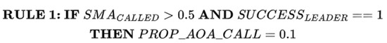
Figure 2. RULE 1 for switching between EAO and LS.

The second rule is formulated to verify whether LS has failed to find a new leader. Consequently, the second rule will be implemented, as shown in Figure 3. In other words, if LS is called most of the time during the update of slime positions and fails to find a new leader, then EAO will be given a high opportunity to update the slime positions in the next iteration.

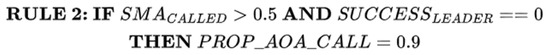
Figure 3. RULE 2 for switching between EAO and LS.

The third rule is designed to verify whether EAO is often called during the update of slime positions and succeeds in finding a new leader. Then, EAO will be given a high chance to continue updating the slime positions in the next iteration. In that case, the third rule will be applied as given in Figure 4.

Figure 4. RULE 3 for switching between EAO and LS.

The fourth rule is developed to verify whether EAO is often called during the update of slime positions and fails to find a new leader. Consequently, LS will have a high probability of updating the slime positions in the next iteration. In this instance, the fourth rule shown in Figure 5 will be applied.

Figure 5. RULE 4 for switching between EAO and LS.

The complete steps of the proposed S²SMA algorithm are given in Algorithm 1 and Figure 6.

Algorithm 1: Pseudo-code of proposed method

Input$: UB, LB,$$max\text{\_}t$$, popsize$ and $\mathrm{n}$. $\mathrm{Initialize} \mathrm{the} \mathrm{parameters} popsize$$, max\text{\_}t$; $\mathrm{Initialize} \mathrm{the} \mathrm{positions} \mathrm{of} \mathrm{slime} \mathrm{molds} X_{\mathrm{i}}\left(\mathrm{i}=1,2,\dots ,\mathrm{n}\right)$; While $(t\le max\text{\_}t)$ Calculate the fitness of all slime molds; $\mathrm{Update} \mathrm{bestFitness},X_b, SUCCES{S}_{LEADER}$; Calculate the $W$ by Equation (5); For $\mathrm{each} \mathrm{slime}$ do If$(r_1<z$) then $\mathrm{Update} \mathrm{the} \mathrm{position} \mathrm{vector} \overrightarrow{X\left(t+1\right)}\mathrm{by} \mathrm{Equation} \left(7\right)$; Else $\mathrm{Update} p,vb, vc$; $\mathrm{Update} \mathrm{prob}\text{\_}\mathrm{AOA}\text{\_}\mathrm{call} \mathrm{using} \mathrm{Apply} \mathrm{embedded} \mathrm{rules}$; For each dimension do If ($rand$$< PROP\text{\_}AOA\text{\_}CALL$) then $\mathrm{Update} \mathrm{the} \mathrm{position} \mathrm{vector} \overrightarrow{X\left(t+1\right)} \mathrm{by} \mathrm{Equation} \left(10\right)$; Else$\mathbf{if} (r_2<p$) then $\mathrm{Update} \mathrm{the} \mathrm{position} \mathrm{vector} \overrightarrow{X\left(t+1\right)} \mathrm{by} \mathrm{Equation} \left(7\right)$; Else $\mathrm{Update} \mathrm{the} \mathrm{position} \mathrm{vector} \overrightarrow{X\left(t+1\right)} \mathrm{by} \mathrm{Equation} \left(8\right)$; End If End $For$ End If End $For$ $t=t+1$; End While Output: $\mathrm{bestFitness},$ $X_{best}$;

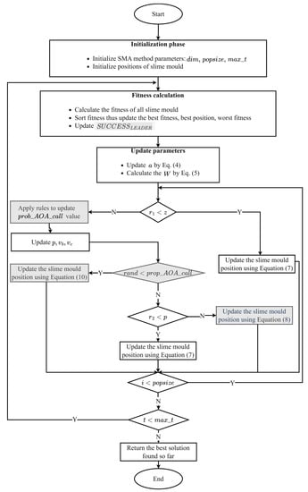
Figure 6. Flow chart of the proposed method.

3.3. Fine-Tuning of Pre-Trained Deep-Face Sketch Using S²SMA

The proposed S²SMA optimization algorithm was integrated with several deep-face models to perform the task of face sketch recognition. This work is divided into two sections: the first section uses a single deep-face model to address face sketch recognition problems and the second combines four deep models to further enhance the recognition performance.

3.3.1. Fine-Tuning of Single Pre-Trained Deep Models

Figure 7 shows the main procedures of fine-tuning a single deep-face model. As indicated, there are three stages, which are feature extraction, feature tuning, and fitness evaluation. In the first stage, all training sketches and the corresponding photos have their features extracted and converted into output vectors. The size of the output vector depends on the model used. In this study, four models were used: FaceNet [21], ArcFace [22], VGG-Face [23], and DeepFace [24]. It is important to note that the output vector size for each deep-face model is different: 128, 512, 2622, and 4096, respectively, as can be seen in Figure 7; note that the feature array has two dimensions, $M$ and $N$, where $M$ represents the number of training images and $N$ represents the number of features in each image (e.g., if we have 10 training images, then the feature array will contain 20 vectors: 10 pairs of sketches and their corresponding photos).

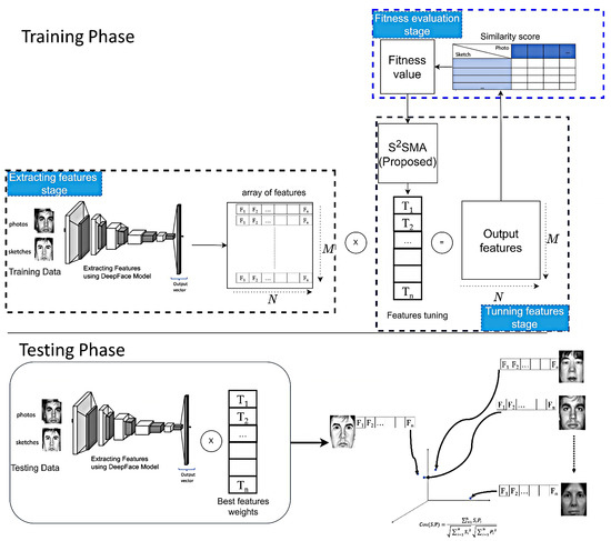
Figure 7. The illustration shows the suggested technique for face sketch recognition using a single deep-face model. The upper portion represents the training phase, while the lower portion represents the testing phase.

In the second stage, S²SMA will generate a “features tuning” vector with random values between 1 and 2. The size of the features tuning vector and the output vector are similar. The output vector and the features tuning vector will be multiplied (element by element), and the result will be saved in the output features array. In other words, there are a lot of features in each image, but there are some features that have a greater impact during the face sketch recognition process for each model. S²SMA attempts to discover the effectiveness of all features and their impact on performance during face sketch recognition. Thus, the optimizer has tuned the features based on how much they are affected. It is worth noting that all deep-face models mentioned above are dedicated only to face recognition [25]. As a result, the suggested algorithm tuned the deep-face models to make them suitable for face sketch recognition.

Finally, based on the features tuned in the previous step, the final step calculates the similarities between each sketch and all photos. This study computes the similarity task using the cosine distance measure, which is defined in Equation (12):

$$\mathrm{Cos}\left(\mathrm{S},\mathrm{P}\right)=\frac{{{\displaystyle \sum }}_{\mathrm{i}=1}^{\mathrm{N}}{\mathrm{S}}_{\mathrm{i}}{\mathrm{P}}_{\mathrm{i}}}{\sqrt{{{\displaystyle \sum }}_{\mathrm{i}=1}^{\mathrm{N}}{\mathrm{S}}_{\mathrm{i}}{}^2}\sqrt{{{\displaystyle \sum }}_{\mathrm{i}=1}^{\mathrm{N}}{\mathrm{P}}_{\mathrm{i}}{}^2}}$$

(12)

where $\mathrm{Cos}$ is the cosine similarity measure. Variables $\mathrm{S}$ and $\mathrm{P}$ represent the input feature vector from the input sketched image and the photo, respectively. Subsequently, the $\mathrm{fitness}$ is calculated based on separation using Equation (13):

$$\mathrm{fitness}=-1\ast \left(\mathrm{mean}\text{\_}\mathrm{seperation}\right)$$

(13)

where $\mathrm{mean}\text{\_}\mathrm{seperation}$ denotes the distance between the input sketch and the nearest incorrect photo, as depicted in Figure 8, where S²SMA aims to maximize this distance. Moreover, every agent will repeat the second and third steps.

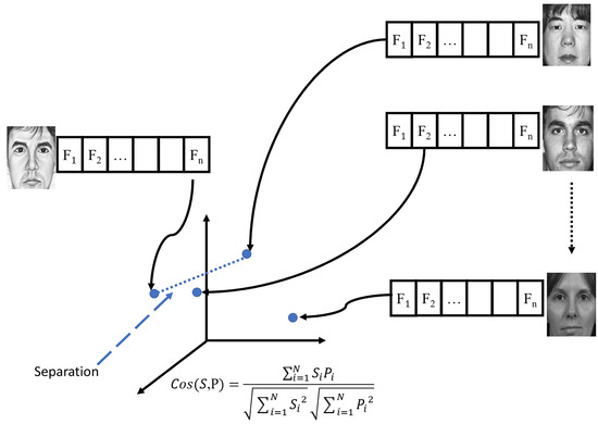
Figure 8. Description of separation measures.

3.3.2. Fine-Tuning of Multiple Pre-Trained Deep Models

As can be seen from Figure 9, which shows the main procedures of the second section, there are four stages in this section: feature extraction, feature tuning, similarity tuning, and fitness evaluation. Overall, this section has four main differences that distinguish it from the previous section. The first difference is that all features are extracted from four different deep-face models simultaneously, each working separately. The models are FaceNet [21], ArcFace [22], VGG-Face [23], and DeepFace [24], and their respective abbreviations are M1, M2, M3, and M4. The second difference, as shown in Figure 9, is that S²SMA will generate a “features tuning” vector divided into four parts; each model has its part (e.g., if M1 has a vector length of 128, then its part is the same length). Next, S²SMA tunes each model’s output vectors, as explained in the previous section. This process is done for each model separately. Then, the results of each model will be saved to the output feature array for that model. The third difference shows that S²SMA also generates a ‘similarity weight’ vector for tuning the model similarities. The vector of similarity weight has four values, W1, W2, W3, and W4, and the values range between [0.1, 1]. These weights are dynamically adjusted using S²SMA, which finds the optimal weights. In other words, S²SMA attempts to find the effectiveness of each model in terms of its accuracy in face sketch recognition. As a result, S²SMA tunes the similarities for each model. The last difference demonstrates how to calculate the average similarity for all four models after tuning similarity, which is calculated based on Equation (14):

$$\begin{array}{c}\mathrm{Cos}\left(\mathrm{S},\mathrm{P}\right)=\mathrm{Average}({\mathrm{W}}_1.\frac{{{\displaystyle \sum }}_{\mathrm{i}=1}^{\mathrm{N}}\mathrm{S}\text{\_}{\mathrm{F}}_{\mathrm{i}}\mathrm{P}\text{\_}{\mathrm{F}}_{\mathrm{i}}}{\sqrt{{{\displaystyle \sum }}_{\mathrm{i}=1}^{\mathrm{N}}\mathrm{S}\text{\_}{\mathrm{F}}_{\mathrm{i}}{}^2}\sqrt{{{\displaystyle \sum }}_{\mathrm{i}=1}^{\mathrm{N}}\mathrm{P}\text{\_}{\mathrm{F}}_{\mathrm{i}}{}^2}}+{\mathrm{W}}_2. \frac{{{\displaystyle \sum }}_{\mathrm{i}=1}^{\mathrm{N}}\mathrm{S}\text{\_}{\mathrm{A}}_{\mathrm{i}}\mathrm{P}\text{\_}{\mathrm{A}}_{\mathrm{i}}}{\sqrt{{{\displaystyle \sum }}_{\mathrm{i}=1}^{\mathrm{N}}\mathrm{S}\text{\_}{\mathrm{A}}_{\mathrm{i}}{}^2}\sqrt{{{\displaystyle \sum }}_{\mathrm{i}=1}^{\mathrm{N}}\mathrm{P}\text{\_}{\mathrm{A}}_{\mathrm{i}}{}^2}}+{\mathrm{W}}_3.\frac{{{\displaystyle \sum }}_{\mathrm{i}=1}^{\mathrm{N}}\mathrm{S}\text{\_}{\mathrm{V}}_{\mathrm{i}}\mathrm{P}\text{\_}{\mathrm{V}}_{\mathrm{i}}}{\sqrt{{{\displaystyle \sum }}_{\mathrm{i}=1}^{\mathrm{N}}\mathrm{S}\text{\_}{\mathrm{V}}_{\mathrm{i}}{}^2}\sqrt{{{\displaystyle \sum }}_{\mathrm{i}=1}^{\mathrm{N}}\mathrm{P}\text{\_}{\mathrm{V}}_{\mathrm{i}}{}^2}}+\\ {\mathrm{W}}_4.\frac{{{\displaystyle \sum }}_{\mathrm{i}=1}^{\mathrm{N}}\mathrm{S}\text{\_}{\mathrm{D}}_{\mathrm{i}}\mathrm{P}\text{\_}{\mathrm{D}}_{\mathrm{i}}}{\sqrt{{{\displaystyle \sum }}_{\mathrm{i}=1}^{\mathrm{N}}\mathrm{S}\text{\_}{\mathrm{D}}_{\mathrm{i}}{}^2}\sqrt{{{\displaystyle \sum }}_{\mathrm{i}=1}^{\mathrm{N}}\mathrm{P}\text{\_}{\mathrm{D}}_{\mathrm{i}}{}^2}})\end{array}$$

(14)

where $\mathrm{Cos}$ is the cosine similarity measure. Variables $\mathrm{S}\text{\_}\mathrm{F}$ and $\mathrm{P}\text{\_}\mathrm{F}$ represent the FaceNet input feature vectors from the input sketched image and the photo, respectively. $\mathrm{S}\text{\_}\mathrm{A}$ and $\mathrm{P}\text{\_}\mathrm{A}$ are ArcFace features, $\mathrm{S}\text{\_}\mathrm{V}$ and $\mathrm{P}\text{\_}\mathrm{V}$ are VGG-Face features, and $\mathrm{S}\text{\_}\mathrm{D}$ and $\mathrm{P}\text{\_}\mathrm{D}$ are DeepFace features.

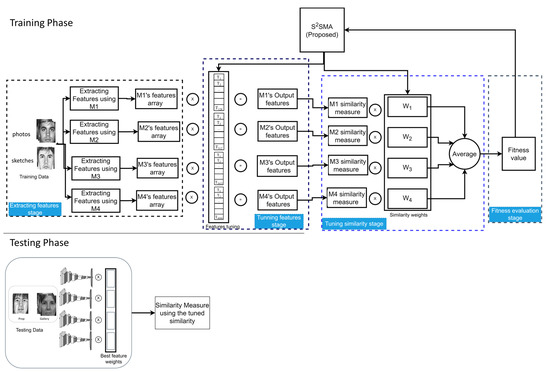
Figure 9. The illustration shows the suggested technique for face sketch recognition using multiple models. The upper portion represents the training phase, while the lower portion represents the testing phase.

4. Experimental Results and Analysis

In this section of the analysis, a series of experiments were performed to verify the efficiency of S²SMA. A total of three case studies were investigated, including large-scale benchmark problems, CEC’2010 benchmark [64], and two public sketch databases, XM2VTS [65] and CUFSF [66].

4.1. Evaluation on Large-Scale Benchmark Problems (CEC’2010)

The usefulness of embedding rules and operations to strengthen the SMA (i.e., the proposed method) on large-scale benchmark issues is investigated in this experimental part. Twenty large-scale functions from the CEC’2010 benchmark functions [64] have specifically been utilized. Table 1 presents details about these functions, namely, separable functions, single-group $m$–non-separable functions, $\frac{\mathrm{D}}{2\mathrm{m}}$ group $m$–non-separable functions, $\frac{\mathrm{D}}{\mathrm{m}}$ group $m$–non-separable functions, and fully separable functions are the five sets of functions that make up the CEC’2010 benchmark.

Table 1. Description of 1000-D CEC’2010 large-scale benchmark functions.

Type	Function	Description	Dim	$\mathbf{Range} [{\mathit{X}}_{\mathit{m}\mathit{i}\mathit{n}}$$, {\mathit{X}}_{\mathit{m}\mathit{a}\mathit{x}}$	${\mathit{f}}_{\mathit{m}\mathit{i}\mathit{n}}\left(\mathit{F}\left(\mathit{X}\right)\right)$
Separable functions	${\mathrm{F}}_1\left(\mathrm{X}\right)={\displaystyle {\displaystyle \sum }_{\mathrm{i}=1}^{\mathrm{D}}}{\left({10}^6\right)}^{\frac{\mathrm{i}-1}{\mathrm{D}-1}}{ \mathrm{Z}}_{\mathrm{i}}^2$	Shifted Elliptic Function	1000	[−100, 100]	0
	${\mathrm{F}}_2\left(\mathrm{X}\right)={\displaystyle {\displaystyle \sum }_{\mathrm{i}=1}^{\mathrm{D}}}\left[{\mathrm{Z}}_{\mathrm{i}}^2-10\cos \left(2{\mathsf{\pi }\mathrm{Z}}_{\mathrm{i}}\right)+10\right]$	Shifted Rastrigin’s Function	1000	[−5, 5]	0
	${\mathrm{F}}_3\left(\mathrm{X}\right)=-20\exp \left(-0.2\sqrt{\frac{1}{\mathrm{D}}{\displaystyle {\displaystyle \sum }_{\mathrm{i}=1}^{\mathrm{D}}}{\mathrm{Z}}_{\mathrm{i}}^2}\right)-\exp \left(\frac{1}{\mathrm{D}}{\displaystyle {\displaystyle \sum }_{\mathrm{i}=1}^{\mathrm{D}}}\cos \left(2{\mathsf{\pi }\mathrm{Z}}_{\mathrm{i}}\right)\right)+20+\mathrm{e}$	Shifted Ackley’s Function	1000	[−32, 32]	0
Single-group m–non-separable functions	${\mathrm{F}}_4\left(\mathrm{X}\right)={\mathrm{F}}_{\mathrm{rot}\text{\_}\mathrm{elliptic}}\left[\mathrm{Z}\left({\mathrm{P}}_1:{\mathrm{P}}_{\mathrm{m}}\right)\right]\ast {10}^6+{\mathrm{F}}_{\mathrm{elliptic}}\left[\mathrm{Z}\left({\mathrm{P}}_{\mathrm{m}+1}:{\mathrm{P}}_{\mathrm{D}}\right)\right]$	Single-group Shifted and m-rotated Elliptic Function	1000	[−100, 100]	0
	${\mathrm{F}}_5\left(\mathrm{X}\right)={\mathrm{F}}_{\mathrm{rot}\text{\_}\mathrm{rastrigin}}\left[\mathrm{Z}\left({\mathrm{P}}_1:{\mathrm{P}}_{\mathrm{m}}\right)\right]\ast {10}^6+{\mathrm{F}}_{\mathrm{rastrigin}}\left[\mathrm{Z}\left({\mathrm{P}}_{\mathrm{m}+1}:{\mathrm{P}}_{\mathrm{D}}\right)\right]$	Single-group Shifted and m-rotated Rastrigin’s Function	1000	[−5, 5]	0
	${\mathrm{F}}_6\left(\mathrm{X}\right)={\mathrm{F}}_{\mathrm{rot}\text{\_}\mathrm{ackley}}\left[\mathrm{Z}\left({\mathrm{P}}_1:{\mathrm{P}}_{\mathrm{m}}\right)\right]\ast {10}^6+{\mathrm{F}}_{\mathrm{ackley}}\left[\mathrm{Z}\left({\mathrm{P}}_{\mathrm{m}+1}:{\mathrm{P}}_{\mathrm{D}}\right)\right]$	Single-group Shifted and m-rotated Ackley’s Function	1000	[−32, 32]	0
	${\mathrm{F}}_7\left(\mathrm{X}\right)={\mathrm{F}}_{\mathrm{schwefel}}\left[\mathrm{Z}\left({\mathrm{P}}_1:{\mathrm{P}}_{\mathrm{m}}\right)\right]\ast {10}^6+{\mathrm{F}}_{\mathrm{sphere}}\left[\mathrm{Z}\left({\mathrm{P}}_{\mathrm{m}+1}:{\mathrm{P}}_{\mathrm{D}}\right)\right]$	Single-group Shifted m-dimensional Schwefel’s	1000	[−100, 100]	0
	${\mathrm{F}}_8\left(\mathrm{X}\right)={\mathrm{F}}_{\mathrm{rosenbrock}}\left[\mathrm{Z}\left({\mathrm{P}}_1:{\mathrm{P}}_{\mathrm{m}}\right)\right]\ast {10}^6+{\mathrm{F}}_{\mathrm{sphere}}\left[\mathrm{Z}\left({\mathrm{P}}_{\mathrm{m}+1}:{\mathrm{P}}_{\mathrm{D}}\right)\right]$	Single-group Shifted m-dimensional Rosenbrock’s Function	1000	[−100, 100]	0
$\frac{\mathrm{D}}{2\mathrm{m}}$ group m–non-separable functions	${\mathrm{F}}_9\left(\mathrm{X}\right)={\displaystyle \sum }_{\mathrm{k}=1}^{\frac{\mathrm{D}}{2\mathrm{m}}}{\mathrm{F}}_{\mathrm{rot}\text{\_}\mathrm{elliptic}}\left[\mathrm{z}\left({\mathrm{P}}_{\left(\mathrm{k}-1\right)\ast \mathrm{m}+1}:{\mathrm{P}}_{\mathrm{k}\ast \mathrm{m}}\right)\right]+{\mathrm{F}}_{\mathrm{elliptic}}\left[\mathrm{z}\left({\mathrm{P}}_{\frac{\mathrm{D}}{2}+1}:{\mathrm{P}}_{\mathrm{D}}\right)\right]$	$\frac{\mathrm{D}}{2\mathrm{m}}$ group Shifted and m-rotated Elliptic Function	1000	[−100, 100]	0
	${\mathrm{F}}_{10}\left(\mathrm{X}\right)={\displaystyle {\displaystyle \sum }_{\mathrm{k}=1}^{\frac{\mathrm{D}}{2\mathrm{m}}}}{\mathrm{F}}_{\mathrm{rot}\text{\_}\mathrm{rastrigin}}\left[\mathrm{z}\left({\mathrm{P}}_{\left(\mathrm{k}-1\right)\ast \mathrm{m}+1}:{\mathrm{P}}_{\mathrm{k}\ast \mathrm{m}}\right)\right]+{\mathrm{F}}_{\mathrm{rastrigin}}\left[\mathrm{z}\left({\mathrm{P}}_{\frac{\mathrm{D}}{2}+1}:{\mathrm{P}}_{\mathrm{D}}\right)\right]$	$\frac{\mathrm{D}}{2\mathrm{m}}$ group Shifted and m-rotated Rastrigin’s Function	1000	[−5, 5]	0
	${\mathrm{F}}_{11}\left(\mathrm{X}\right)={\displaystyle {\displaystyle \sum }_{\mathrm{k}=1}^{\frac{\mathrm{D}}{2\mathrm{m}}}}{\mathrm{F}}_{\mathrm{rot}\text{\_}\mathrm{ackley}}\left[\mathrm{z}\left({\mathrm{P}}_{\left(\mathrm{k}-1\right)\ast \mathrm{m}+1}:{\mathrm{P}}_{\mathrm{k}\ast \mathrm{m}}\right)\right]+{\mathrm{F}}_{\mathrm{ackley}}\left[\mathrm{z}\left({\mathrm{P}}_{\frac{\mathrm{D}}{2}+1}:{\mathrm{P}}_{\mathrm{D}}\right)\right]$	$\frac{\mathrm{D}}{2\mathrm{m}}$ group Shifted and m-rotated Ackley’s Function	1000	[−32, 32]	0
	${\mathrm{F}}_{12}\left(\mathrm{X}\right)={\displaystyle {\displaystyle \sum }_{\mathrm{k}=1}^{\frac{\mathrm{D}}{2\mathrm{m}}}}{\mathrm{F}}_{\mathrm{schwefel}}\left[\mathrm{z}\left({\mathrm{P}}_{\left(\mathrm{k}-1\right)\ast \mathrm{m}+1}:{\mathrm{P}}_{\mathrm{k}\ast \mathrm{m}}\right)\right]+{\mathrm{F}}_{\mathrm{sphere}}\left[\mathrm{z}\left({\mathrm{P}}_{\frac{\mathrm{D}}{2}+1}:{\mathrm{P}}_{\mathrm{D}}\right)\right]$	$\frac{\mathrm{D}}{2\mathrm{m}}$ group Shifted m-rotated Schwefel’s	1000	[−100, 100]	0
	${\mathrm{F}}_{13}\left(\mathrm{X}\right)={\displaystyle {\displaystyle \sum }_{\mathrm{k}=1}^{\frac{\mathrm{D}}{2\mathrm{m}}}}{\mathrm{F}}_{\mathrm{rosenbrock}}\left[\mathrm{z}\left({\mathrm{P}}_{\left(\mathrm{k}-1\right)\ast \mathrm{m}+1}:{\mathrm{P}}_{\mathrm{k}\ast \mathrm{m}}\right)\right]+{\mathrm{F}}_{\mathrm{sphere}}\left[\mathrm{z}\left({\mathrm{P}}_{\frac{\mathrm{D}}{2}+1}:{\mathrm{P}}_{\mathrm{D}}\right)\right]$	$\frac{\mathrm{D}}{2\mathrm{m}}$ group Shifted m-rotated Rosenbrock’s Function	1000	[−100, 100]	0
$\frac{D}{m}$ group m–non-separable functions	${\mathrm{F}}_{14}\left(\mathrm{X}\right)={\displaystyle {\displaystyle \sum }_{\mathrm{k}=1}^{\frac{\mathrm{D}}{\mathrm{m}}}}{\mathrm{F}}_{\mathrm{rot}\text{\_}\mathrm{elliptic}}\left[\mathrm{z}\left({\mathrm{P}}_{\left(\mathrm{k}-1\right)\ast \mathrm{m}+1}:{\mathrm{P}}_{\mathrm{k}\ast \mathrm{m}}\right)\right]$	$\frac{\mathrm{D}}{\mathrm{m}}$ group Shifted and m-rotated Elliptic Function	1000	[−100, 100]	0
	${\mathrm{F}}_{15}\left(\mathrm{X}\right)={\displaystyle {\displaystyle \sum }_{\mathrm{k}=1}^{\frac{\mathrm{D}}{\mathrm{m}}}}{\mathrm{F}}_{\mathrm{rot}\text{\_}\mathrm{rastrigin}}\left[\mathrm{z}\left({\mathrm{P}}_{\left(\mathrm{k}-1\right)\ast \mathrm{m}+1}:{\mathrm{P}}_{\mathrm{k}\ast \mathrm{m}}\right)\right]$	$\frac{\mathrm{D}}{\mathrm{m}}$ group Shifted and m-rotated Rastrigin’s Function	1000	[−5, 5]	0
	${\mathrm{F}}_{16}\left(\mathrm{X}\right)={\displaystyle {\displaystyle \sum }_{\mathrm{k}=1}^{\frac{\mathrm{D}}{\mathrm{m}}}}{\mathrm{F}}_{\mathrm{rot}\text{\_}\mathrm{ackley}}\left[\mathrm{z}\left({\mathrm{P}}_{\left(\mathrm{k}-1\right)\ast \mathrm{m}+1}:{\mathrm{P}}_{\mathrm{k}\ast \mathrm{m}}\right)\right]$	$\frac{\mathrm{D}}{\mathrm{m}}$ group Shifted and m-rotated Ackley’s Function	1000	[−32, 32]	0
	${\mathrm{F}}_{17}\left(\mathrm{X}\right)={\displaystyle {\displaystyle \sum }_{\mathrm{k}=1}^{\frac{\mathrm{D}}{\mathrm{m}}}}{\mathrm{F}}_{\mathrm{schwefel}}\left[\mathrm{z}\left({\mathrm{P}}_{\left(\mathrm{k}-1\right)\ast \mathrm{m}+1}:{\mathrm{P}}_{\mathrm{k}\ast \mathrm{m}}\right)\right]$	$\frac{\mathrm{D}}{\mathrm{m}}$ group Shifted m-rotated Schwefel	1000	[−100, 100]	0
	${\mathrm{F}}_{18}\left(\mathrm{X}\right)={\displaystyle {\displaystyle \sum }_{\mathrm{k}=1}^{\frac{\mathrm{D}}{\mathrm{m}}}}{\mathrm{F}}_{\mathrm{rosenbrock}}\left[\mathrm{z}\left({\mathrm{P}}_{\left(\mathrm{k}-1\right)\ast \mathrm{m}+1}:{\mathrm{P}}_{\mathrm{k}\ast \mathrm{m}}\right)\right]$	$\frac{\mathrm{D}}{\mathrm{m}}$ group Shifted m-rotated Rosenbrock’s Function	1000	[−100, 100]	0
Fully separable functions	${\mathrm{F}}_{19}\left(\mathrm{X}\right)={\displaystyle {\displaystyle \sum }_{\mathrm{i}=1}^{\mathrm{n}}}{\left({\displaystyle {\displaystyle \sum }_{\mathrm{j}=1}^{\mathrm{i}}}{\mathrm{x}}_{\mathrm{i}}\right)}^2$	Shifted Schwefel’s	1000	[−100, 100]	0
	${\mathrm{F}}_{20}\left(\mathrm{X}\right)={\displaystyle {\displaystyle \sum }_{\mathrm{i}=1}^{\mathrm{D}-1}}\left[100{\left({\mathrm{z}}_{\mathrm{i}}^2-{\mathrm{z}}_{\mathrm{i}+1}\right)}^2+{\left({\mathrm{z}}_{\mathrm{i}}-1\right)}^2\right]$	Shifted Rosenbrock’s Function	1000	[−100, 100]	0

4.1.1. The Influence of Population Size

This section examines the impact of population size on S²SMA’s performance. In total, 2 experiments with populations of 10 and 30 were conducted for comparison and analysis. As shown in Table 2, the search accuracy of S²SMA tends to decrease when a small population is used, i.e., ten agents. This result is because a greater number gives the potential to discover more regions than a smaller number, thus finding the best solution. Based on this finding, 30 agents have been utilized in the remaining experiments.

Table 2. Comparison of S²SMA (proposed) with 10 and 30 search agents.

Function	Algorithm
	Proposed_30	Proposed_10	Proposed_30	Proposed_10
	Mean	Mean	Std.	Std.
F1	8.8 × 109	2.26 × 1010	6.57 × 108	1.58 × 109
F2	12,129.97	13,175.47	198.788	219.3744
F3	20.97428	20.98415	0.014797	0.016608
F4	3.82 × 1013	6.92 × 1013	1.32 × 1013	1.93 × 1013
F5	2.71 × 108	3.45 × 108	55,552,821	91,773,918
F6	5,113,851	11,026,896	4,929,368	6,083,478
F7	5.69 × 109	2.32 × 1010	1.51 × 109	4.59 × 109
F8	1.37 × 109	1.04 × 1010	2.59 × 109	1.18 × 1010
F9	1.14 × 1010	2.47 × 1010	5.67 × 108	1.99 × 109
F10	12,130.43	13,041.73	178.6562	185.0105
F11	227.1399	228.2753	0.659421	0.635519
F12	3,809,917	4,223,945	189,280.9	230,020.6
F13	3.76 × 109	5.52 × 1010	6.97 × 108	8.12 × 109
F14	1.28 × 1010	2.6 × 1010	1.25 × 109	2.09 × 109
F15	12,230.97	13,068.63	189.9647	222.8522
F16	412.4328	414.7671	0.712702	0.882251
F17	4,775,455	5,446,786	316,617.3	457,231.5
F18	1.25 × 1011	4.27 × 1011	1.46 × 1010	2.98 × 1010
F19	13,908,503	19,032,212	1,323,228	1,332,130
F20	1.52 × 1011	5.05 × 1011	1.26 × 1010	3.31 × 1010

4.1.2. Performance Analysis

This section aims to compare the performance of S²SMA against SMA [28], AOA [59], and recently developed SMA variants. Specifically, LSMA [36], AOSMA [37], and ESMA [56] are executed based on the settings indicated in Table 3. Table 4 presents the results of comparisons between all algorithms for the best, median, worst, mean, and standard deviation. An average of 30 runs were used to determine the ranking. The outcomes show that S²SMA surpassed all other algorithms in most functions. This is because S²SMA can converge quickly and switch to exploitation mode faster. However, the results in single-group m–non-separable functions were not satisfactory. Nevertheless, F8 in this group demonstrates S²SMA ‘s superiority over other algorithms, and F4’s algorithm results in the same group were comparable to those of the other algorithms.

Table 3. Parameter settings for the studied algorithms.

Algorithm	Population	Maximum No. of Iterations	Parameter Settings
S2SMA (proposed)	30	${10}^3$	$z$ = 0.03, $\mathsf{\alpha }$ = 5, $\mu$ = 0.5, and $\beta$ = 3/2
SMA [28]	30	${10}^3$	$z$ = 0.03
ESMA [56]	30	${10}^3$	$z$ = 0.03
LSMA [36]	30	${10}^3$	$z$ = 0.03
AOSMA [37]	30	${10}^3$	$z$ = 0.03
AOA [59]	30	${10}^3$	$\alpha$= 5 and $\mu$ = 0.5

Table 4. Results of 1000-D CEC’2010 large-scale functions.

Function	Fitness	Algorithm
		S2SMA (Proposed)	SMA	ESMA	LSMA	AOSMA	AOA
F1	Best	1.76 × 109	7.81 × 109	5.14 × 109	1.11 × 1010	1.57 × 1010	1.77 × 1011
	Median	2.06 × 109	9.14 × 109	6.03 × 109	1.4 × 1010	1.88 × 1010	1.88 × 1011
	Worst	2.61 × 109	1.05 × 1010	6.89 × 109	1.54 × 1010	2.27 × 1010	1.98 × 1011
	Mean	2.07 × 109	9.17 × 109	5.95 × 109	1.37 × 1010	1.87 × 1010	1.88 × 1011
	Std	1.98 × 108	7.18 × 108	4.63 × 108	1 × 109	1.85 × 109	4.99 × 109
F2	Best	7420.003	11,622.23	11,122.65	11,563.58	12,220.17	16,814.9
	Median	7913.024	12,123.91	11,553.64	12,078.19	12,808.79	16,879.47
	Worst	8543.541	12,562.58	11,909.94	12,525.94	13,488.04	16,928.68
	Mean	7914.655	12,094.01	11,540.2	12,044.08	12,862.12	16,880.43
	Std	223.0079	233.6023	177.2629	227.6748	289.5164	25.38681
F3	Best	20.45723	20.94333	20.94137	20.82354	20.74332	20.96937
	Median	20.53913	20.97172	20.97353	20.87073	20.88426	20.97909
	Worst	20.62014	20.99172	20.99089	20.90363	20.94046	20.98651
	Mean	20.5377	20.97023	20.97294	20.8696	20.87993	20.97899
	Std	0.034483	0.011155	0.010779	0.019869	0.045559	0.004683
F4	Best	1.98 × 1013	2.3 × 1013	1.96 × 1013	1.62 × 1013	2.63 × 1013	6.05 × 1014
	Median	4.46 × 1013	4.24 × 1013	3.76 × 1013	3.83 × 1013	5.7 × 1013	1.72 × 1015
	Worst	7.16 × 1013	6.28 × 1013	5.32 × 1013	6.36 × 1013	1 × 1014	3.26 × 1015
	Mean	4.38 × 1013	4.2 × 1013	3.76 × 1013	3.92 × 1013	5.67 × 1013	1.81 × 1015
	Std	1.39 × 1013	1.1 × 1013	8.79 × 1012	1.09 × 1013	1.97 × 1013	6.56 × 1014
F5	Best	3.87 × 108	1.45 × 108	1.35 × 108	1.3 × 108	2.32 × 108	6.56 × 108
	Median	4.63 × 108	2.68 × 108	2.39 × 108	2.35 × 108	3.53 × 108	7.37 × 108
	Worst	6.57 × 108	4.66 × 108	4.53 × 108	4.66 × 108	4.67 × 108	8.18 × 108
	Mean	4.93 × 108	2.75 × 108	2.59 × 108	2.47 × 108	3.53 × 108	7.31 × 108
	Std	78,930,465	70,779,121	72,072,794	76,161,679	66,866,994	42,197,174
F6	Best	19,092,882	2,667,085	2,211,587	3,267,670	7,694,194	19,871,195
	Median	19,283,502	3,444,805	3,135,796	4,676,409	17,075,574	20,205,266
	Worst	19,623,059	19,549,466	19,242,111	8,729,924	19,638,217	20,456,178
	Mean	19,303,738	4,156,635	3,825,783	4,731,126	16,199,990	20,209,715
	Std	126,238.1	2,994,700	2,983,575	1,109,918	3,183,234	137,216.6
F7	Best	1.75 × 1010	2.33 × 109	2.18 × 109	5.69 × 109	1.25 × 1010	2.45 × 1011
	Median	2.96 × 1010	5.38 × 109	4.86 × 109	1.1 × 1010	2.44 × 1010	1.52 × 1012
	Worst	4.51 × 1010	9.66 × 109	8.37 × 109	1.69 × 1010	3.44 × 1010	4.28 × 1012
	Mean	2.91 × 1010	5.64 × 109	4.74 × 109	1.07 × 1010	2.41 × 1010	1.65 × 1012
	Std	6.34 × 109	1.77 × 109	1.5 × 109	2.53 × 109	5.9 × 109	9.14 × 1011
F8	Best	44,622,771	1.85 × 108	1.01 × 108	74,068,916	3.83 × 108	3.06 × 1016
	Median	1.87 × 108	3.65 × 108	4.48 × 108	7.17 × 108	1.69 × 109	4.83 × 1016
	Worst	8.21 × 109	9.81 × 109	1.05 × 1010	1.04 × 1010	9.92 × 109	6.05 × 1016
	Mean	8.02 × 108	1.92 × 109	2.08 × 109	2.37 × 109	2.85 × 109	4.88 × 1016
	Std	1.61 × 109	2.92 × 109	3.12 × 109	3.17 × 109	2.79 × 109	7.63 × 1015
F9	Best	4.07 × 109	9.71 × 109	7.34 × 109	1.37 × 1010	1.63 × 1010	2.1 × 1011
	Median	4.62 × 109	1.12 × 1010	8.6 × 109	1.6 × 1010	2.05 × 1010	2.22 × 1011
	Worst	5.47 × 109	1.36 × 1010	9.8 × 109	1.86 × 1010	2.55 × 1010	2.35 × 1011
	Mean	4.62 × 109	1.13 × 1010	8.62 × 109	1.6 × 1010	2.05 × 1010	2.23 × 1011
	Std	2.81 × 108	8.49 × 108	6.85 × 108	1.01 × 109	2.17 × 109	7.27 × 109
F10	Best	9874.878	11,724.88	11,405.84	11,488.99	11,704.62	16,819.37
	Median	10,182.29	12,223.82	11,845.07	11,925.26	12,586.2	17,079.4
	Worst	10,664.76	12,635.02	12,259.19	12,260.33	13,429.73	17,306.07
	Mean	10,201.98	12,226.61	11,853.7	11,917.62	12,551.05	17,081.76
	Std	189.7485	226.7152	211.632	197.3043	422.7365	118.8733
F11	Best	219.4078	225.7075	225.7055	223.557	222.9627	229.0635
	Median	221.713	228.3196	226.8211	225.1769	225.684	229.757
	Worst	224.0152	229.8544	229.3891	226.6153	227.2091	230.1152
	Mean	221.6478	228.1962	227.105	225.1461	225.4392	229.725
	Std	1.239087	1.205704	0.982233	0.735506	1.106646	0.26831
F12	Best	2,276,120	3,368,692	3,030,133	3,851,178	3,849,260	12,102,047
	Median	2,621,306	3,728,335	3,327,312	4,225,549	4,752,430	15,370,248
	Worst	2,882,778	4,160,006	3,906,673	4,682,711	5,508,701	21,048,071
	Mean	2,620,532	3,730,252	3,412,245	4,254,445	4,686,477	15,602,565
	Std	130,216.5	175,431.2	238,544.8	206,243.5	404,333	2,239,131
F13	Best	2.02 × 108	2.71 × 109	1 × 109	9.99 × 109	2.3 × 1010	6.7 × 1011
	Median	2.9 × 108	3.83 × 109	1.48 × 109	1.45 × 1010	3.08 × 1010	6.84 × 1011
	Worst	5.68 × 108	5.67 × 109	1.94 × 109	1.79 × 1010	4.67 × 1010	6.96 × 1011
	Mean	3.18 × 108	3.87 × 109	1.48 × 109	1.45 × 1010	3.14 × 1010	6.83 × 1011
	Std	86,911,529	6.78 × 108	2.76 × 108	2.11 × 109	5.13 × 109	7.06 × 109
F14	Best	5.74 × 109	1.12 × 1010	8.94 × 109	1.47 × 1010	1.85 × 1010	2.19 × 1011
	Median	7.16 × 109	1.28 × 1010	1.06 × 1010	1.63 × 1010	2.19 × 1010	2.45 × 1011
	Worst	9.41 × 109	1.47 × 1010	1.22 × 1010	1.94 × 1010	2.37 × 1010	2.6 × 1011
	Mean	7.26 × 109	1.28 × 1010	1.06 × 1010	1.63 × 1010	2.14 × 1010	2.45 × 1011
	Std	8.9 × 108	9.49 × 108	9.58 × 108	1.04 × 109	1.54 × 109	9.83 × 109
F15	Best	10,441.07	11,715.81	11,521.83	11,414.74	11,608.27	16,581.15
	Median	10,943.73	12,247.13	11,915.48	11,756.24	12,400.18	16,868.84
	Worst	11,704.28	12,656.63	12,463.85	12,280.87	12,949.81	17,125.66
	Mean	10,960.73	12,246.81	11,898.22	11,767.4	12,358.15	16,884.21
	Std	254.8337	262.1877	233.1186	215.1636	381.2675	137.7109
F16	Best	404.6271	410.8071	411.5858	408.5032	409.4019	417.1974
	Median	408.1271	413.8228	413.8984	409.986	413.1222	417.7382
	Worst	410.3292	416.0813	415.0011	413.5427	414.788	418.3869
	Mean	407.8513	413.7724	413.679	410.2303	412.7576	417.7455
	Std	1.285974	1.20194	0.926444	1.286516	1.445627	0.267426
F17	Best	2,466,681	3,951,118	3,821,661	4,715,783	4,548,857	33,001,378
	Median	3,731,849	4,476,318	4,312,100	5,214,502	5,499,177	43,564,464
	Worst	4,662,725	5,232,786	4,966,740	5,797,767	6,587,557	51,734,401
	Mean	3,533,019	4,512,265	4,311,666	5,217,711	5,541,469	43,619,099
	Std	541,249.5	291,273.4	276,255	290,986.3	545,820.7	5,020,599
F18	Best	2.95 × 1010	9.7 × 1010	5.49 × 1010	1.69 × 1011	2.63 × 1011	1.44 × 1012
	Median	3.62 × 1010	1.17 × 1011	7.61 × 1010	2.05 × 1011	3.07 × 1011	1.46 × 1012
	Worst	4.19 × 1010	1.4 × 1011	8.61 × 1010	2.43 × 1011	3.52 × 1011	1.47 × 1012
	Mean	3.63 × 1010	1.17 × 1011	7.5 × 1010	2.07 × 1011	3.07 × 1011	1.46 × 1012
	Std	3.28 × 109	1.09 × 1010	7.55 × 109	1.83 × 1010	2.33 × 1010	6.02 × 109
F19	Best	9,885,192	11,537,452	11,829,648	11,496,363	13,366,719	45,969,764
	Median	11,948,149	13,796,444	13,120,993	15,140,891	19,832,030	75,940,439
	Worst	16,032,746	16,494,867	17,101,180	17,142,757	24,729,783	1.15 × 108
	Mean	12,263,206	13,961,159	13,262,631	14,884,574	19,471,422	75,902,843
	Std	1,588,291	1,332,594	1,048,934	1,322,939	2,358,851	18,375,810
F20	Best	3.69 × 1010	1.2 × 1011	7.77 × 1010	2.29 × 1011	3.29 × 1011	1.62 × 1012
	Median	4.58 × 1010	1.47 × 1011	9.26 × 1010	2.59 × 1011	3.8 × 1011	1.64 × 1012
	Worst	6.45 × 1010	1.84 × 1011	1.08 × 1011	2.95 × 1011	4.3 × 1011	1.65 × 1012
	Mean	4.76 × 1010	1.48 × 1011	9.31 × 1010	2.62 × 1011	3.81 × 1011	1.64 × 1012
	Std	6.68 × 109	1.42 × 1010	8.43 × 109	1.61 × 1010	2.59 × 1010	7.39 × 109

4.1.3. Convergence Evaluation

In this section, Figure 10 depicts the convergence graphs between S²SMA and the original SMA [28], AOA [59], and SMA variants (LSMA [36], AOSMA [37], and ESMA [56]), which are compared in Table 4. The convergence curves in Figure 10 are based on the mean value of the best objective function obtained after 30 runs. The horizontal axis represents the number of iterations, ${10}^3$, while the vertical axis represents the highest score obtained. As seen in all functions, the convergence is far better in S²SMA than in other algorithms in most functions. It can be seen in Figure 10 that S²SMA has a much faster convergence speed than the original SMA and others. This is due to the ability of S²SMA to switch to exploitation mode early in the search process and LF’s ability to avoid falling into the local optima.

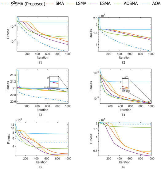
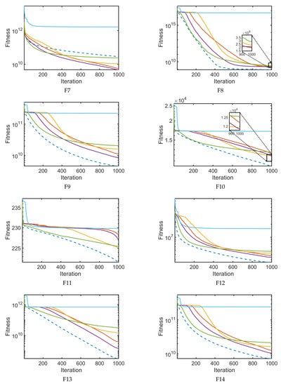
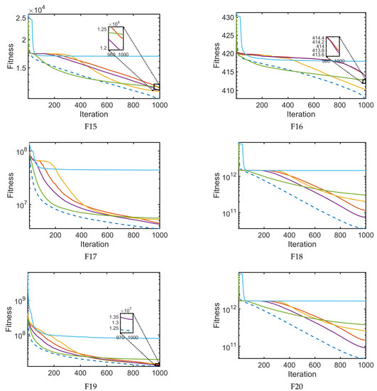
Figure 10. The convergence curves for large-scale functions F1–F20.

4.1.4. Statistical Analysis

To statistically evaluate the performance of S²SMA compared to the original SMA, AOA, and SMA variants (LSMA, AOSMA, and ESMA), the p-value of the Wilcoxon signed-rank test [67] is computed. Each value above 0.05 is displayed in bold to indicate that the difference is not statistically significant. As shown in Table 5, S²SMA is significantly better than other algorithms on the majority of test problems. This shows that the original SMA’s capability for exploration and exploitation has been significantly enhanced by the addition of embedded rules and operations. However, F4, F5, F6, and F7 yielded no satisfactory results, showing that the difference compared to the proposed approach is not statistically significant. In contrast, S²SMA outperformed every other algorithm in the remaining functions.

Table 5. p-values for S²SMA versus other competitors on a large scale.

Function No.	SMA	ESMA	LSMA	AOSMA	AOA
1	3.02 × 10−11	3.02 × 10−11	3.02 × 10−11	3.02 × 10−11	3.02 × 10−11
2	3.02 × 10−11	3.02 × 10−11	3.02 × 10−11	3.02 × 10−11	3.02 × 10−11
3	3.02 × 10−11	3.02 × 10−11	3.02 × 10−11	3.02 × 10−11	3.02 × 10−11
4	0.630876	0.082357	0.17145	0.011711	3.02 × 10−11
5	1	1	1	1	1
6	1	1	1	0.999999	1
7	1	1	1	0.992383	1
8	0.001857	0.009883	0.000377	2.88 × 10−6	3.02 × 10−11
9	3.02 × 10−11	3.02 × 10−11	3.02 × 10−11	3.02 × 10−11	3.02 × 10−11
10	3.02 × 10−11	3.02 × 10−11	3.02 × 10−11	3.02 × 10−11	3.02 × 10−11
11	3.02 × 10−11	3.02 × 10−11	3.02 × 10−11	3.02 × 10−11	3.02 × 10−11
12	3.02 × 10−11	3.02 × 10−11	3.02 × 10−11	3.02 × 10−11	3.02 × 10−11
13	3.02 × 10−11	3.02 × 10−11	3.02 × 10−11	3.02 × 10−11	3.02 × 10−11
14	3.02 × 10−11	3.02 × 10−11	3.02 × 10−11	3.02 × 10−11	3.02 × 10−11
15	3.02 × 10−11	3.02 × 10−11	3.02 × 10−11	3.02 × 10−11	3.02 × 10−11
16	3.02 × 10−11	3.02 × 10−11	1.85 × 10−08	3.02 × 10−11	3.02 × 10−11
17	3.82 × 10−10	7.77 × 10−09	3.02 × 10−11	3.02 × 10−11	3.02 × 10−11
18	3.02 × 10−11	3.02 × 10−11	3.02 × 10−11	3.02 × 10−11	3.02 × 10−11
19	9.79 × 10−5	0.005084	3.26 × 10−7	3.02 × 10−11	3.02 × 10−11
20	3.02 × 10−11	3.02 × 10−11	3.02 × 10−11	3.02 × 10−11	3.02 × 10−11

4.1.5. Execution Time Analysis

The software and hardware specifications of the computer used for conducting the experiments in this study are listed in Table 6. This section compares the computational time of S²SMA with that of SMA for large-scale problems. This investigation was performed to determine the overhead related to the embedded rules and operations, shown in Table 7. The average computation time for 30 iterations of the F1 function is provided in Table 7. Clearly, S²SMA required more time due to the calculations of population status and agent location required to execute the embedded rules and operations. However, the computational time required by these rules and operations is reasonable, at less than one second. This value accounts for approximately 7% of the overall time required by SMA. It should be noted that the CPU time consumed by each method is affected by several factors, such as programming language, programming skill, and hardware configuration.

Table 6. The details of hardware and software settings.

Item	Component	Setting
Hardware	CPU	Intel(R) Core (TM) i7-10700
	Frequency	2.9 GHz
	RAM	16GB
	GPU	Nvidia GeForce GTX 1660 Super
	SSD	256 GB
	Hard Drive	2 TB
Software	Operating System	Windows 10
	Language	MATLAB R2021a

Table 7. Computational time analysis.

	SMA	S2SMA (Proposed)
Time (second)	13.51	12.54

4.2. Evaluation on Face Sketch Recognition

This section evaluates the effectiveness of S²SMA for fine-tuning several pre-trained deep models in handling the face sketch recognition problem. A total of two public datasets were used to evaluate the performances, including XM2VTS [65] and CUFSF [66]. It should be noted that these datasets have been utilized frequently in the literature [25], [68,69]. Partition settings of images contained in each database are shown in Table 8. As in earlier research [1,25], each database was separated into training and testing, as indicated in Table 8. Some example images from XM2VTS and CUFSF are displayed in Figure 11. It is worth mentioning that the datasets were taken without any image enhancements or pre-processing. S²SMA was run 10 times for each dataset with a population size set to 30, and the maximum number of iterations is ${10}^3$.

Table 8. The studied database sketches.

Database	Number of Sketch–Photo Pairs	Training Pairs	Testing Pairs
XM2VTS	295	100	195
CUFSF	1194	955	239

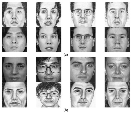
Figure 11. Sample images from (a) XM2VTS database, and (b) CUFSF database.

4.2.1. Case Study I: XM2VTS Dataset

XM2VTS [65] database was used to evaluate the efficiency of S²SMA in fine-tuning pre-trained deep models. The features were extracted in two ways: using single deep-face models and a multiple deep-face model, as shown previously in the methodology section. In this study, a total of four deep models were used, which are FaceNet [21], ArcFace [22], VGG-Face [23], and DeepFace [24].

The Mean Recognition Rates

This experiment evaluates the performance of S²SMA compared to the original SMA [28], AOA [59], and SMA variants (LSMA [36], AOSMA [37], and ESMA [56]) on face sketch recognition. Table 9 summarizes the mean recognition rate from rank 1 to 10 for XM2VTS. The results were compared using single-model and multiple-model approaches. The proposed model achieved the highest recognition rate at rank 1 among other algorithms and was non-optimized in all experiments. For example, it outperforms rank 1 with 98.81% in multiple-model tests, while the single-model tests closest to it, FaceNet and ArcFace, scored 85.28%. Table 9 also shows that S²SMA reported a 100% accurate recognition rate at rank 2 in multiple-model tests, exceeding other results obtained. The results can be attributed to the efficiency of S²SMA in tuning multiple-model features based on their importance and giving weight to each model based on its efficiency.

Table 9. A comparison of the effectiveness of several optimization algorithms and a non-optimized model on XMTVTS.

Deep-Face Model	Algorithm	Accuracy (%)
		Rank 1	Rank 2	Rank 3	Rank 4	Rank 5	Rank 6	Rank 7	Rank 8	Rank 9	Rank 10
Facenet	S2SMA (proposed)	85.28	91.28	94.56	96.15	97.08	97.49	98.21	98.72	98.92	99.13
	SMA [28]	83.79	91.13	94.26	95.85	96.82	97.69	97.95	98.26	98.46	98.67
	ESMA [56]	84.67	90.67	94.00	95.74	96.92	97.38	97.95	98.15	98.36	98.46
	LSMA [36]	84.46	91.08	94.82	96.36	97.38	98.00	98.46	98.82	99.03	99.23
	AOSMA [37]	83.79	90.77	94.26	95.79	96.87	97.49	97.85	98.10	98.51	98.77
	AOA [59]	83.38	91.33	94.00	95.49	96.56	97.18	97.44	97.95	98.10	98.56
	Non-optimized	84.62	90.77	93.85	95.90	96.92	97.95	98.46	98.46	98.46	98.46
ArcFace	S2SMA (proposed)	85.28	93.13	97.03	97.95	98.67	99.13	99.33	99.49	99.49	99.59
	SMA	84.72	93.18	96.36	96.92	98.00	98.36	98.67	98.87	99.28	99.38
	ESMA	84.87	93.18	96.51	97.28	98.10	98.51	98.82	99.03	99.33	99.44
	LSMA	84.36	92.31	96.26	97.54	98.26	98.46	99.03	99.13	99.18	99.23
	AOSMA	84.15	92.10	96.05	97.54	97.95	98.51	99.03	99.18	99.18	99.44
	AOA	83.28	92.92	95.74	97.33	98.10	98.67	98.82	98.97	99.13	99.18
	Non-optimized	84.10	93.33	97.44	97.44	98.46	98.46	98.46	98.97	99.49	99.49
VGG-Face	S2SMA (proposed)	72.82	84.51	90.26	92.51	94.26	94.72	95.33	96.92	97.49	97.95
	SMA	71.44	82.77	89.03	91.38	93.49	94.26	94.97	96.05	96.87	97.74
	ESMA	71.79	82.87	88.82	91.69	93.54	94.26	94.82	95.95	96.92	97.79
	LSMA	71.59	82.97	88.41	91.38	93.38	94.15	94.87	96.15	96.77	97.74
	AOSMA	71.28	83.44	88.92	91.49	93.28	94.31	94.92	96.21	97.03	97.90
	AOA	72.10	83.59	89.28	91.90	93.59	94.26	95.08	96.36	97.08	97.74
	Non-optimized	71.28	82.05	89.74	91.28	93.33	93.85	94.36	96.41	96.92	97.95
DeepFace	S2SMA (proposed)	41.85	54.36	59.38	64.41	68.62	71.85	74.87	76.51	77.85	79.03
	SMA	40.62	52.26	57.18	62.51	67.08	71.08	74.05	76.05	77.38	78.36
	ESMA	41.13	52.31	56.92	61.44	66.77	70.72	73.18	75.54	77.18	78.36
	LSMA	40.92	52.41	57.33	62.56	67.38	71.13	73.79	76.15	77.64	78.87
	AOSMA	41.13	52.05	57.44	63.08	67.49	70.46	73.85	75.69	77.18	78.36
	AOA	41.28	52.77	58.67	63.74	67.49	70.67	73.38	75.79	77.49	78.77
	Non-optimized	41.03	51.79	56.92	62.05	67.18	70.77	75.38	76.92	78.97	79.49
Multiple-model	S2SMA (proposed)	98.92	100.00	100.00	100.00	100.00	100.00	100.00	100.00	100.00	100.00
	SMA	97.85	99.85	99.95	100.00	100.00	100.00	100.00	100.00	100.00	100.00
	ESMA	97.74	99.79	99.90	99.95	100.00	100.00	100.00	100.00	100.00	100.00
	LSMA	98.41	99.85	99.95	100.00	100.00	100.00	100.00	100.00	100.00	100.00
	AOSMA	98.62	100.00	100.00	100.00	100.00	100.00	100.00	100.00	100.00	100.00
	AOA	97.85	99.85	100.00	100.00	100.00	100.00	100.00	100.00	100.00	100.00
	Non-optimized	97.95	100.00	100.00	100.00	100.00	100.00	100.00	100.00	100.00	100.00

The Cumulative Matching Characteristic

Further study was performed by calculating the cumulative matching characteristic (CMC) generated by S²SMA vs. the non-optimized model for FaceNet, ArcFace, VGG-Face, DeepFace, and multiple-model, as given in Figure 12. CMC evaluates face sketch recognition performance along an x-axis ranging from 1 to $k$. The y-axis displays the recognition rate for each rank value. As demonstrated in Figure 12, S²SMA had a better recognition curve for most ranks between 1 and 10 in all models. Furthermore, as shown in Figure 12, S²SMA achieved 100% precision in multiple-model at rank 2. Moreover, at the level of single-model, S²SMA at rank 1 outperformed the non-optimized in all models.

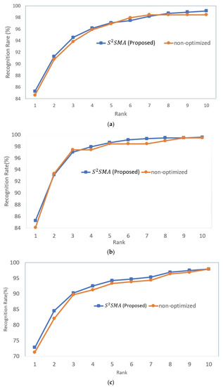
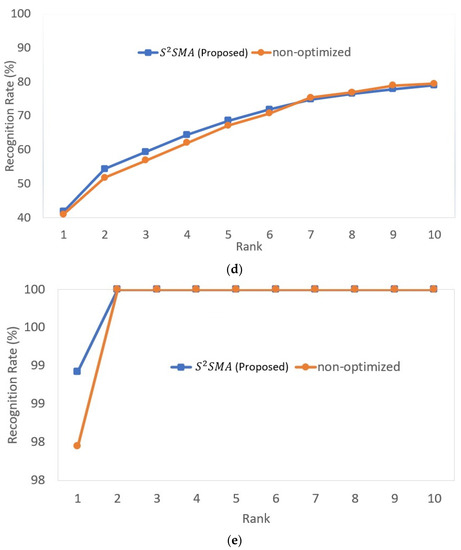
Figure 12. The CMC results of S²SMA as compared with non-optimized for (a) FaceNet, (b) ArcFace, (c) VGG-Face, (d) DeepFace, and (e) multiple-model.

Fitness Value Analysis

This section aims to compare the performance of S²SMA compared to the original SMA [28], AOA [59], and SMA variants (LSMA [36], AOSMA [37], and ESMA [56]). Table 10 includes the results of the single-model and multiple-model approaches. Table 10 shows the best, worst, average, and mean of all algorithms, as well as the standard deviation. S²SMA received the highest mean value for both single-model and multiple-model approaches out of all the other algorithms. For example, the best mean value for a multiple-model is S²SMA, with a value of −2.34 × 10⁻¹. On the other hand, the worst mean value for the multiple-model approach is ESMA, with a value of −1.77 × 10⁻¹, the lowest among all algorithms.

Table 10. The fitness outcomes of several single-model and multiple-model approaches on XMTVTS.

Deep-Face Model	Fitness	Algorithm
		S2SMA (Proposed)	SMA	ESMA	LSMA	AOSMA	AOA
FaceNet	Best	−9.53 × 10−2	−5.94 × 10−2	−5.91 × 10−2	−8.28 × 10−2	−8.17 × 10−2	−7.02 × 10−2
	Median	−9.42 × 10−2	−5.72 × 10−2	−5.79 × 10−2	−7.95 × 10−2	−7.92 × 10−2	−6.51 × 10−2
	Worst	−9.16 × 10−2	−5.61 × 10−2	−5.59 × 10−2	−7.63 × 10−2	−7.77 × 10−2	−6.37 × 10−2
	Mean	−9.41 × 10−2	−5.74 × 10−2	−5.77 × 10−2	−7.92 × 10−2	−7.95 × 10−2	−6.61 × 10−2
	Std	1.04 × 10−3	1.03 × 10−3	1.16 × 10−3	2.24 × 10−3	1.25 × 10−3	2.23 × 10−3
ArcFace	Best	−7.95 × 10−2	−5.16 × 10−2	−5.27 × 10−2	−5.92 × 10−2	−6.08 × 10−2	−5.62 × 10−2
	Median	−7.79 × 10−2	−5.09 × 10−2	−5.14 × 10−2	−5.60 × 10−2	−5.77 × 10−2	−5.38 × 10−2
	Worst	−7.69 × 10−2	−5.05 × 10−2	−5.10 × 10−2	−5.34 × 10−2	−5.58 × 10−2	−5.23 × 10−2
	Mean	−7.80 × 10−2	−5.10 × 10−2	−5.17 × 10−2	−5.60 × 10−2	−5.78 × 10−2	−5.41 × 10−2
	Std	8.60 × 10−4	4.02 × 10−4	6.74 × 10−4	2.04 × 10−3	1.56 × 10−3	1.14 × 10−3
VGG-Face	Best	−2.57 × 10−2	−1.65 × 10−2	−1.64 × 10−2	−1.72 × 10−2	−1.75 × 10−2	−1.73 × 10−2
	Median	−2.54 × 10−2	−1.60 × 10−2	−1.61 × 10−2	−1.67 × 10−2	−1.69 × 10−2	−1.70 × 10−2
	Worst	−2.51 × 10−2	−1.58 × 10−2	−1.59 × 10−2	−1.62 × 10−2	−1.65 × 10−2	−1.67 × 10−2
	Mean	−2.54 × 10−2	−1.61 × 10−2	−1.61 × 10−2	−1.67 × 10−2	−1.69 × 10−2	−1.70 × 10−2
	Std	2.25 × 10−4	2.29 × 10−4	1.88 × 10−4	2.86 × 10−4	3.34 × 10−4	2.05 × 10−4
DeepFace	Best	−1.34 × 10−2	−6.82 × 10−3	−6.84 × 10−3	−7.65 × 10−3	−7.69 × 10−3	−7.93 × 10−3
	Median	−1.31 × 10−2	−6.46 × 10−3	−6.54 × 10−3	−7.01 × 10−3	−7.20 × 10−3	−7.46 × 10−3
	Worst	−1.28 × 10−2	−6.21 × 10−3	−6.30 × 10−3	−6.50 × 10−3	−6.79 × 10−3	−7.33 × 10−3
	Mean	−1.31 × 10−2	−6.47 × 10−3	−6.54 × 10−3	−7.01 × 10−3	−7.19 × 10−3	−7.53 × 10−3
	Std	1.63 × 10−4	1.72 × 10−4	1.67 × 10−4	4.01 × 10−4	3.10 × 10−4	1.77 × 10−4
Multiple-model	Best	−2.37 × 10−1	−1.85 × 10−1	−1.84 × 10−1	−2.20 × 10−1	−2.26 × 10−1	−1.87 × 10−1
	Median	−2.33 × 10−1	−1.78 × 10−1	−1.75 × 10−1	−2.14 × 10−1	−2.17 × 10−1	−1.86 × 10−1
	Worst	−2.31 × 10−1	−1.76 × 10−1	−1.74 × 10−1	−2.06 × 10−1	−2.12 × 10−1	−1.82 × 10−1
	Mean	−2.34 × 10−1	−1.79 × 10−1	−1.77 × 10−1	−2.14 × 10−1	−2.18 × 10−1	−1.85 × 10−1
	Std	1.86 × 10−3	3.02 × 10−3	3.44 × 10−3	4.89 × 10−3	3.93 × 10−3	1.68 × 10−3

Convergence Evaluation

Further investigation was done by analysing the convergence graphs between S²SMA and other algorithms used in Table 10 and plotted in Figure 13. As shown in Figure 13, S²SMA has the fastest and most effective convergence speed, outperforming all other optimizers for single-model and multiple-model face sketch recognition. This demonstrates that S²SMA is capable of addressing large-scale problems. In other words, the ability of all single-model and multiple-model approaches to converge has been greatly improved by tuning features and similarity and by combining all deep-face models.

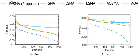
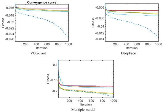
Figure 13. The convergence curves for several single-model and multiple-model approaches.

Statistical Analysis

To statistically evaluate the performance of S²SMA compared to other algorithms, the p-value of the Wilcoxon signed-rank test [67] is computed. As shown in Table 11, S²SMA is significantly better than other algorithms on all test problems. This shows that the original SMA’s capability for exploration and exploitation has been significantly enhanced by the addition of embedded rules and operations.

Table 11. p-values for S²SMA versus other competitors on XM2VTS.

Algorithm	FaceNet	ArcFace	VGG-Face	DeepFace	Multiple-Model
SMA	1.83 × 10-4	1.83 × 10-4	1.83 × 10-4	1.83 × 10-4	1.83 × 10-4
ESMA	1.83 × 10-4	1.83 × 10-4	1.83 × 10-4	1.83 × 10-4	1.83 × 10-4
LSMA	1.83 × 10-4	1.83 × 10-4	1.83 × 10-4	1.83 × 10-4	1.83 × 10-4
AOSMA	1.83 × 10-4	1.83 × 10-4	1.83 × 10-4	1.83 × 10-4	1.83 × 10-4
AOA	1.83 × 10-4	1.83 × 10-4	1.83 × 10-4	1.83 × 10-4	1.83 × 10-4

4.2.2. Case Study II: CUFSF Dataset

In this section, the CUFSF database was used to evaluate the efficiency of S²SMA. The features were extracted from multiple deep-face models, as explained previously in the methodology section.

The Mean Recognition Rates

This experiment compares the face sketch recognition performance of S²SMA with that of the original SMA [28], AOA [59], and SMA variants (LSMA [36], AOSMA [37], and ESMA [56]). Table 12 summarizes the average recognition rate from rank 1 to 10 for CUFSF. The findings were compared using multiple model approaches, as demonstrated in Table 12. Moreover, the fine-tuned model was compared with the non-optimized model (non-fine-tuned). The results clearly showed that S²SMA achieved the highest recognition rate at rank 1 with 75.82%. This is owing to the benefits of the embedded rules and operations explained in Section 4.1. On the other hand, ESMA [56] had the lowest rank 1 performance in this experiment, with a percentage of 74.35%.

Table 12. Comparison of the effectiveness of several optimization model algorithms and the non-optimized model on CUFSF.

Algorithm	Accuracy (%)
	Rank 1	Rank 2	Rank 3	Rank 4	Rank 5	Rank 6	Rank 7	Rank 8	Rank 9	Rank 10
S2SMA (Proposed)	75.82	84.10	86.40	88.08	88.79	89.29	89.54	89.79	90.04	90.50
SMA	74.52	83.77	86.07	87.74	88.49	88.91	89.12	89.83	89.92	90.08
ESMA	74.35	83.85	86.15	87.91	88.62	89.00	89.21	90.00	90.04	90.13
LSMA	75.31	84.35	86.40	87.78	88.58	88.95	89.33	89.83	90.13	90.54
AOSMA	75.27	83.97	86.07	87.53	88.37	89.21	89.46	89.87	90.29	90.63
AOA	75.31	83.51	85.61	87.32	88.37	89.00	89.50	89.75	90.04	90.50
non-optimized	74.90	84.94	86.61	88.28	88.70	89.12	89.12	89.96	89.96	89.96

The Cumulative Matching Characteristic

Further research was conducted by calculating the cumulative matching characteristic (CMC) obtained by the suggested model in comparison to the non-optimized model for the multiple-model approach. As indicated in Figure 14, along an x-axis ranging from 1 to $k$, CMC measures face sketch recognition performance. The y-axis represents the recognition rate for every rank value. Figure 14 demonstrates that the proposed model has a better recognition curve for the majority of rankings between 1 and 10 in the multiple-model approach.

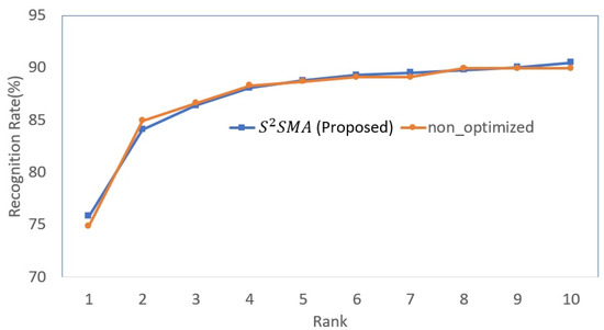
Figure 14. The CMC results of the proposed method as compared with the non-optimized multiple-model approach.

Fitness Value Analysis

This section compares the fitness of S²SMA with the original SMA, AOA, and SMA variations (LSMA, AOSMA, and ESMA) when it is applied for fine-tuning of multiple deep-face models. Table 13 contains the multiple-model results, showing each algorithm’s best, worst, average, mean, and standard deviation. Table 13 summarizes the obtained mean value from 30 independent runs. As can be seen, S²SMA obtained the greatest mean value among all other algorithms. For instance, the optimal mean value for S²SMA is −1.94 × 10⁻¹. Conversely, the worst mean value for the multiple-model technique is −1.55 × 10⁻¹ for ESMA, which is the lowest among all algorithms.

Table 13. Multiple-model fitness results on CUFSF.

Fitness	Algorithm
	S2SMA (Proposed)	SMA	ESMA	LSMA	AOSMA	AOA
Best	−1.98 × 10−1	−1.60 × 10−1	−1.59 × 10−1	−1.83 × 10−1	−1.85 × 10−1	−1.66 × 10−1
Median	−1.94 × 10−1	−1.55 × 10−1	−1.54 × 10−1	−1.78 × 10−1	−1.82 × 10−1	−1.61 × 10−1
Worst	−1.89 × 10−1	−1.54 × 10−1	−1.54 × 10−1	−1.75 × 10−1	−1.75 × 10−1	−1.59 × 10−1
Mean	−1.94 × 10−1	−1.56 × 10−1	−1.55 × 10−1	−1.79 × 10−1	−1.81 × 10−1	−1.62 × 10−1
Std	2.65 × 10−3	1.92 × 10−3	1.42 × 10−3	2.86 × 10−3	3.24 × 10−3	2.14 × 10−3

Comparison with the Reported Results

The proposed face sketch recognition model is compared with previously reported results by other related methods on the CUFUS dataset. Table 14 compares the recognition results’ rank 1 accuracies. As can be seen, the suggested method achieves a rank 1 recognition accuracy value of 75.82, exceeding all competing methods. This is due the advantage of combining the features of several deep models and tuning them using S²SMA.

Table 14. Accuracy (%) comparisons by different methods on CUFUS.

	HOG [70]	SIFT [71]	DCP [72]	[25]	S2SMA (Proposed)
Rank 1	46.03	41.84	50.21	72.38	75.82

5. Future Perspective of the Research

In this research, S²SMA has been introduced as an enhanced optimization algorithm for deep-face sketch recognition models. The experimental findings show that S²SMA outperforms related algorithms regarding convergence rate and recognition accuracy. Beyond face sketch recognition, there are several potential future applications for S²SMA, including decision-making, finance, feature selection, and image processing. In addition, S²SMA can be expanded to solve additional face recognition problems, and its scalability and efficacy can be studied further by testing it on larger datasets and more complex models. In terms of applications and utility, the proposed S²SMA algorithm has the potential to significantly improve the accuracy of face sketch recognition, which has important implementations in law enforcement, security, and surveillance systems. The ability to recognize faces from sketches can aid in solving crimes and identifying suspects, especially in cases where photographic evidence is unavailable or unreliable. In addition, a hybrid method can be investigated by combining S²SMA with other optimization algorithms to improve its performance.

6. Conclusions

This work introduces an enhanced optimization algorithm named S²SMA, which has been applied for fine-tuning deep-face sketch recognition models. Many techniques were used to enhance the conducted optimizer, including incorporating embedded control and adding new search operations, namely AOA and LF operations. The experimental analysis performed on CEC’s 2010 large-scale benchmark showed that S²SMA significantly outperformed other related algorithms and had a faster convergence rate. Moreover, for the assessment of S²SMA‘s efficiency in face sketch recognition, two databases were used: XM2VTS and CUFSF. In addition, S²SMA has been applied to fine-tune the features of four deep-face models, namely FaceNet, ArcFace, VGG-Face, and DeepFace. The results of the finely tuned deep models were compared with several other models, such as the non-fine-tuned model, as well as with reported results in the literature. The results showed the superiority of S²SMA in all experiments in rank 1. XM2VTS had a 98.81% recognition rate in the multiple-model, while the single-model results closest to it, FaceNet and ArcFace, scored an 85.28% recognition rate. CUFSF achieves a recognition rate of 75.82% in the multiple-model approach. This considerable result is attributable to the better image quality of XM2VTS compared to CUFSF, which is susceptible to various distortions, shape exaggerations, and illumination problems. Finally, the statistical data analysis for all experiments, including the t-test, demonstrated that S²SMA significantly outperformed other algorithms with a confidence level of 95%.

References

- Samma, H.; Suandi, S.A.; Mohamad-Saleh, J. Face sketch recognition using a hybrid optimization model. Neural Comput. Appl. 2019, 31, 6493–6508. [Google Scholar] [CrossRef]
- Radman, A.; Suandi, S.A. A Superpixel-Wise Approach for Face Sketch Synthesis. IEEE Access 2019, 7, 108838–108849. [Google Scholar] [CrossRef]
- Radman, A.; Suandi, S.A. BiLSTM regression model for face sketch synthesis using sequential patterns. Neural Comput. Appl. 2021, 33, 12689–12702. [Google Scholar] [CrossRef]
- Radman, A.; Suandi, S.A. Robust face pseudo-sketch synthesis and recognition using morphological-arithmetic operations and HOG-PCA. Multimed. Tools Appl. 2018, 77, 25311–25332. [Google Scholar] [CrossRef]
- Radman, A.; Sallam, A.; Suandi, S.A. Deep residual network for face sketch synthesis. Expert Syst. Appl. 2022, 190, 115980. [Google Scholar] [CrossRef]
- Galea, C.; Farrugia, R.A. Matching Software-Generated Sketches to Face Photographs with a Very Deep CNN, Morphed Faces, and Transfer Learning. IEEE Trans. Inf. Forensics Secur. 2018, 13, 1421–1431. [Google Scholar] [CrossRef]
- Liu, D.; Gao, X.; Wang, N.; Peng, C.; Li, J. Iterative local re-ranking with attribute guided synthesis for face sketch recognition. Pattern Recognit. 2021, 109, 107579. [Google Scholar] [CrossRef]
- Qi, X.; Sun, M.; Wang, W.; Dong, X.; Li, Q.; Shan, C. Face Sketch Synthesis via Semantic-Driven Generative Adversarial Network. In Proceedings of the International Joint Conference on Biometrics (IJCB), Shenzhen, China, 4–7 August 2021; pp. 1–8. [Google Scholar]
- Bae, S.; Din, N.U.; Park, H.; Yi, J. Face Photo-Sketch Recognition Using Bidirectional Collaborative Synthesis Network. In Proceedings of the 16th International Conference on Ubiquitous Information Management and Communication (IMCOM), Seoul, Republic of Korea, 3–5 January 2022; pp. 1–8. [Google Scholar]
- Wan, W.; Lee, H.J. Generative adversarial multi-task learning for face sketch synthesis and recognition. In Proceedings of the International Conference on Image Processing, Taipei, Taiwan, 22–25 September 2019; pp. 4065–4069. [Google Scholar]
- Tu, C.-T.; Chan, Y.-H.; Chen, Y.-C. Facial Sketch Synthesis Using 2D Direct Combined Model-Based Face-Specific Markov Network. IEEE Trans. Image Process. 2016, 25, 3546–3561. [Google Scholar] [CrossRef]
- Kan, M.; Shan, S.; Zhang, H.; Lao, S.; Chen, X. Multi-view discriminant analysis. IEEE Trans. Pattern Anal. Mach. Intell. 2015, 38, 188–194. [Google Scholar] [CrossRef] [PubMed]
- Huo, J.; Gao, Y.; Shi, Y.; Yin, H. Cross-Modal Metric Learning for AUC Optimization. IEEE Trans. Neural Netw. Learn. Syst. 2018, 29, 4844–4856. [Google Scholar] [CrossRef]
- Han, H.; Klare, B.F.; Bonnen, K.; Jain, A.K. Matching Composite Sketches to Face Photos: A Component-Based Approach. IEEE Trans. Inf. Forensics Secur. 2012, 8, 191–204. [Google Scholar] [CrossRef]
- Klare, B.; Li, Z.; Jain, A.K. Matching Forensic Sketches to Mug Shot Photos. IEEE Trans. Pattern Anal. Mach. Intell. 2010, 33, 639–646. [Google Scholar] [CrossRef] [PubMed]
- Huo, J.; Gao, Y.; Shi, Y.; Yang, W.; Yin, H. Heterogeneous Face Recognition by Margin-Based Cross-Modality Metric Learning. IEEE Trans. Cybern. 2017, 48, 1814–1826. [Google Scholar] [CrossRef] [PubMed]
- Xu, J.; Xue, X.; Wu, Y.; Mao, X. Matching a composite sketch to a photographed face using fused HOG and deep feature models. Vis. Comput. 2021, 37, 765–776. [Google Scholar] [CrossRef]
- Bhatt, H.S.; Bharadwaj, S.; Singh, R.; Vatsa, M. Memetically Optimized MCWLD for Matching Sketches with Digital Face Images. IEEE Trans. Inf. Forensics Secur. 2012, 7, 1522–1535. [Google Scholar] [CrossRef]
- Bhatt, H.S.; Bharadwaj, S.; Singh, R.; Vatsa, M. On matching sketches with digital face images. In Proceedings of the 4th IEEE International Conference on Biometrics: Theory, Applications and Systems (BTAS), Washington, DC, USA, 27–29 September 2010. [Google Scholar]
- Samma, H.; Suandi, S.A.; Mohamad-saleh, J. A Hybrid Deep Learning Model for Face Sketch Recognition. In Proceedings of the 11th International Conference on Robotics, Vision, Signal Processing and Power Applications, Penang, Malaysia, 2022; pp. 545–551. [Google Scholar]
- Champandard, A.J. FaceNet: A Unified Embedding for Face Recognition and Clustering. In Proceedings of the Conference on Computer Vision and Pattern Recognition, Boston, MA, USA, 7–12 June 2015; pp. 815–823. [Google Scholar]
- Deng, J.; Guo, J.; Xue, N.; Zafeiriou, S. Arcface: Additive angular margin loss for deep face recognition. In Proceedings of the IEEE/CVF Conference on Computer Vision and Pattern Recognition, Long Beach, CA, USA, 15–20 June 2019; pp. 4690–4699. [Google Scholar]
- Parkhi, O.M.; Vedaldi, A.; Zisserman, A. Deep Face Recognition; University of Oxford: Oxford, UK, 2015. [Google Scholar]
- Taigman, Y.; Yang, M.; Ranzato, M.; Wolf, L. Deepface: Closing the gap to human-level performance in face verification. In Proceedings of the Conference on Computer Vision and Pattern Recognition, Columbus, OH, USA, 23–28 June 2014; pp. 1701–1708. [Google Scholar]
- Wan, W.; Gao, Y.; Lee, H.J. Transfer deep feature learning for face sketch recognition. Neural Comput. Appl. 2019, 31, 9175–9184. [Google Scholar] [CrossRef]
- Abdullah, J.M.; Ahmed, T. Fitness Dependent Optimizer: Inspired by the Bee Swarming Reproductive Process. IEEE Access 2019, 7, 43473–43486. [Google Scholar] [CrossRef]
- Shamsaldin, A.S.; Rashid, T.A.; Agha, R.A.A.-R.; Al-Salihi, N.K.; Mohammadi, M. Donkey and smuggler optimization algorithm: A collaborative working approach to path finding. J. Comput. Des. Eng. 2019, 6, 562–583. [Google Scholar] [CrossRef]
- Li, S.; Chen, H.; Wang, M.; Heidari, A.A.; Mirjalili, S. Slime mould algorithm: A new method for stochastic optimization. Future Gener. Comput. Syst. 2020, 111, 300–323. [Google Scholar] [CrossRef]
- Hayyolalam, V.; Kazem, A.A.P. Black Widow Optimization Algorithm: A novel meta-heuristic approach for solving engineering optimization problems. Eng. Appl. Artif. Intell. 2020, 87, 103249. [Google Scholar] [CrossRef]
- Połap, D.; Woźniak, M. Red fox optimization algorithm. Expert Syst. Appl. 2021, 166, 114107. [Google Scholar] [CrossRef]
- Hamad, Q.S.; Samma, H.; Suandi, S.A.; Mohamad-Saleh, J. Q-learning embedded sine cosine algorithm (QLESCA). Expert Syst. Appl. 2022, 193, 116417. [Google Scholar] [CrossRef]
- Abualigah, L.; Abd Elaziz, M.; Sumari, P.; Geem, Z.W.; Gandomi, A.H. Reptile Search Algorithm (RSA): A nature-inspired meta-heuristic optimizer. Expert Syst. Appl. 2022, 191, 116158. [Google Scholar] [CrossRef]
- Zhao, S.; Wang, P.; Heidari, A.A.; Chen, H.; Turabieh, H.; Mafarja, M.; Li, C. Multilevel threshold image segmentation with diffusion association slime mould algorithm and Renyi’s entropy for chronic obstructive pulmonary disease. Comput. Biol. Med. 2021, 134, 104427. [Google Scholar] [CrossRef]
- Nguyen, T.-T.; Wang, H.-J.; Dao, T.-K.; Pan, J.-S.; Liu, J.-H.; Weng, S. An Improved Slime Mold Algorithm and its Application for Optimal Operation of Cascade Hydropower Stations. IEEE Access 2020, 8, 226754–226772. [Google Scholar] [CrossRef]
- Abualigah, L.; Diabat, A.; Elaziz, M.A. Improved slime mould algorithm by opposition-based learning and Levy flight distribution for global optimization and advances in real-world engineering problems. J. Ambient. Intell. Humaniz. Comput. 2021, 14, 1163–1202. [Google Scholar] [CrossRef]
- Naik, M.K.; Panda, R.; Abraham, A. Normalized square difference based multilevel thresholding technique for multispectral images using leader slime mould algorithm. J. King Saud Univ. Comput. Inf. Sci. 2020, 34, 4524–4536. [Google Scholar] [CrossRef]
- Naik, M.K.; Panda, R.; Abraham, A. Adaptive opposition slime mould algorithm. Soft Comput. 2021, 25, 14297–14313. [Google Scholar] [CrossRef]
- Kundu, T.; Garg, H. LSMA-TLBO: A hybrid SMA-TLBO algorithm with lévy flight based mutation for numerical optimization and engineering design problems. Adv. Eng. Softw. 2022, 172, 103185. [Google Scholar] [CrossRef]
- Hermosilla, G.; Rojas, M.; Mendoza, J.; Farias, G.; Pizarro, F.T.; Martin, C.S.; Vera, E. Particle Swarm Optimization for the Fusion of Thermal and Visible Descriptors in Face Recognition Systems. IEEE Access 2018, 6, 42800–42811. [Google Scholar] [CrossRef]
- Khan, S.A.; Ishtiaq, M.; Nazir, M.; Shaheen, M. Face recognition under varying expressions and illumination using particle swarm optimization. J. Comput. Sci. 2018, 28, 94–100. [Google Scholar] [CrossRef]
- Subramanian, R.R.; Mohan, H.; Jenny, A.M.; Sreshta, D.; Prasanna, M.L.; Mohan, P. PSO Based Fuzzy-Genetic Optimization Technique for Face Recognition. In Proceedings of the 11th International Conference on Cloud Computing, Data Science & Engineering (Confluence), Noida, India, 28–29 January 2021; pp. 374–379. [Google Scholar]
- Ahmed, S.; Frikha, M.; Hussein, T.D.H.; Rahebi, J. Optimum Feature Selection with Particle Swarm Optimization to Face Recognition System Using Gabor Wavelet Transform and Deep Learning. BioMed Res. Int. 2021, 2021, 6621540. [Google Scholar] [CrossRef]
- Chalabi, N.E.; Attia, A.; Bouziane, A.; Akhtar, Z. Particle swarm optimization based block feature selection in face recognition system. Multimed. Tools Appl. 2021, 80, 33257–33273. [Google Scholar] [CrossRef]
- Annamalai, P. Automatic Face Recognition Using Enhanced Firefly Optimization Algorithm and Deep Belief Network. Int. J. Intell. Eng. Syst. 2020, 13, 19–28. [Google Scholar] [CrossRef]
- Ahmed, S.; Frikha, M.; Hussein, T.D.H.; Rahebi, J. Harris Hawks Optimization Method based on Convolutional Neural Network for Face Recognition Systems. In Proceedings of the International Congress on Human-Computer Interaction, Optimization and Robotic Applications (HORA), Ankara, Turkey, 9–11 June 2022; pp. 1–6. [Google Scholar]
- Alsubai, S.; Hamdi, M.; Abdel-Khalek, S.; Alqahtani, A.; Binbusayyis, A.; Mansour, R.F. Bald eagle search optimization with deep transfer learning enabled age-invariant face recognition model. Image Vis. Comput. 2022, 126, 104545. [Google Scholar] [CrossRef]
- Ren, D.; Yang, J.; Wei, Z. Multi-Level Cycle-Consistent Adversarial Networks with Attention Mechanism for Face Sketch-Photo Synthesis. Sensors 2022, 22, 6725. [Google Scholar] [CrossRef] [PubMed]
- Rizkinia, M.; Faustine, N.; Okuda, M. Conditional Generative Adversarial Networks with Total Variation and Color Correction for Generating Indonesian Face Photo from Sketch. Appl. Sci. 2022, 12, 10006. [Google Scholar] [CrossRef]
- Zhong, K.; Chen, Z.; Liu, C.; Wu, Q.M.J.; Duan, S. Unsupervised self-attention lightweight photo-to-sketch synthesis with feature maps. J. Vis. Commun. Image Represent. 2023, 90, 103747. [Google Scholar] [CrossRef]
- Peng, C.; Zhang, C.; Liu, D.; Wang, N.; Gao, X. Face photo-sketch synthesis via intra-domain enhancement. Knowl.-Based Syst. 2023, 259, 110026. [Google Scholar] [CrossRef]
- Peng, Y.; Zhao, C.; Xie, H.; Fukusato, T.; Miyata, K. DiffFaceSketch: High-Fidelity Face Image Synthesis with Sketch-Guided Latent Diffusion Model. arXiv 2023, arXiv:2302.06908. [Google Scholar]
- Singh, A.; Kushwaha, S.; Alarfaj, M.; Singh, M. Comprehensive Overview of Backpropagation Algorithm for Digital Image Denoising. Electronics 2022, 11, 1590. [Google Scholar] [CrossRef]
- Hassan, M.H.; Kamel, S.; Abualigah, L.; Eid, A. Development and application of slime mould algorithm for optimal economic emission dispatch. Expert Syst. Appl. 2021, 182, 115205. [Google Scholar] [CrossRef]
- Liu, L.; Zhao, D.; Yu, F.; Heidari, A.A.; Ru, J.; Chen, H.; Mafarja, M.; Turabieh, H.; Pan, Z. Performance optimization of differential evolution with slime mould algorithm for multilevel breast cancer image segmentation. Comput. Biol. Med. 2021, 138, 104910. [Google Scholar] [CrossRef] [PubMed]
- Lin, H.; Ahmadianfar, I.; Golilarz, N.A.; Jamei, M.; Heidari, A.A.; Kuang, F.; Zhang, S.; Chen, H. Adaptive slime mould algorithm for optimal design of photovoltaic models. Energy Sci. Eng. 2022, 10, 2035–2064. [Google Scholar] [CrossRef]
- Naik, M.K.; Panda, R.; Abraham, A. An entropy minimization based multilevel colour thresholding technique for analysis of breast thermograms using equilibrium slime mould algorithm. Appl. Soft Comput. 2021, 113, 107955. [Google Scholar] [CrossRef]
- Chauhan, S.; Vashishtha, G.; Kumar, A. A symbiosis of arithmetic optimizer with slime mould algorithm for improving global optimization and conventional design problem. J. Supercomput. 2022, 78, 6234–6274. [Google Scholar] [CrossRef]
- Altay, O. Chaotic slime mould optimization algorithm for global optimization. Artif. Intell. Rev. 2022, 55, 3979–4040. [Google Scholar] [CrossRef]
- Abualigah, L.; Diabat, A.; Mirjalili, S.; Abd Elaziz, M.; Gandomi, A.H. The Arithmetic Optimization Algorithm. Comput. Methods Appl. Mech. Eng. 2021, 376, 113609. [Google Scholar] [CrossRef]
- Cui, Z.; Hou, X.; Zhou, H.; Lian, W.; Wu, J. Modified Slime Mould Algorithm via Levy Flight. In Proceedings of the 13th International Congress on Image and Signal Processing, BioMedical Engineering and Informatics (CISP-BMEI 2020), Chengdu, China, 17–19 October 2020; pp. 1109–1113. [Google Scholar]
- Deepa, R.; Venkataraman, R. Enhancing Whale Optimization Algorithm with Levy Flight for coverage optimization in wireless sensor networks. Comput. Electr. Eng. 2021, 94, 107359. [Google Scholar] [CrossRef]
- Iacca, G.; dos Santos Junior, V.C.; Veloso de Melo, V. An improved Jaya optimization algorithm with Lévy flight. Expert Syst. Appl. 2021, 165, 113902. [Google Scholar] [CrossRef]
- Heidari, A.A.; Mirjalili, S.; Faris, H.; Aljarah, I.; Mafarja, M.; Chen, H. Harris hawks optimization: Algorithm and applications. Futur. Gener. Comput. Syst. 2019, 97, 849–872. [Google Scholar] [CrossRef]
- Ke, T.; Li, X.; Omidvar, M.N.; Yang, Z.; Thomas, W. Benchmark Functions for the CEC’2013 Special Session and Competition on Large-Scale Global Optimization; University of Science and Technology of China: Hefei, China, 2010; pp. 1–21. [Google Scholar]
- Messer, K.; Matas, J.; Kittler, J.; Luettin, J.; Maitre, G. XM2VTSDB: The extended M2VTS database. In Proceedings of the 2nd International Conference on Audio and Video-Based Biometric Person Authentication, Washington, DC, USA, 22–24 March 1999; Volume 964, pp. 965–966. [Google Scholar]
- Zhang, W.; Wang, X.; Tang, X. Coupled information-theoretic encoding for face photo-sketch recognition. In Proceedings of the CVPR 2011, Colorado Springs, CO, USA, 20–25 June 2011; pp. 513–520. [Google Scholar]
- García, S.; Fernández, A.; Luengo, J.; Herrera, F. Advanced nonparametric tests for multiple comparisons in the design of experiments in computational intelligence and data mining: Experimental analysis of power. Inf. Sci. 2010, 180, 2044–2064. [Google Scholar] [CrossRef]
- Li, P.; Sheng, B.; Chen, C.L.P. Face Sketch Synthesis Using Regularized Broad Learning System. In IEEE Transactions on Neural Networks and Learning Systems; IEEE: New York, NY, USA, 2021; pp. 5346–5360. [Google Scholar]
- Wang, N.; Gao, X.; Sun, L.; Li, J. Bayesian Face Sketch Synthesis. IEEE Trans. Image Process. 2017, 26, 1264–1274. [Google Scholar] [CrossRef] [PubMed]
- Galoogahi, H.K.; Sim, T. Inter-modality face sketch recognition. In Proceedings of the International Conference on Multimedia and Expo, Melbourne, VIC, Australia, 9–13 July 2012; pp. 224–229. [Google Scholar]
- Lenc, L.; Král, P. Automatic face recognition system based on the SIFT features. Comput. Electr. Eng. 2015, 46, 256–272. [Google Scholar] [CrossRef]
- Ding, C.; Choi, J.; Tao, D.; Davis, L.S. Multi-Directional Multi-Level Dual-Cross Patterns for Robust Face Recognition. IEEE Trans. Pattern Anal. Mach. Intell. 2015, 38, 518–531. [Google Scholar] [CrossRef] [PubMed]
Disclaimer/Publisher’s Note: The statements, opinions and data contained in all publications are solely those of the individual author(s) and contributor(s) and not of MDPI and/or the editor(s). MDPI and/or the editor(s) disclaim responsibility for any injury to people or property resulting from any ideas, methods, instructions or products referred to in the content. |
© 2023 by the authors. Licensee MDPI, Basel, Switzerland. This article is an open access article distributed under the terms and conditions of the Creative Commons Attribution (CC BY) license (https://creativecommons.org/licenses/by/4.0/).