Longitudinal Control Strategy for Connected Electric Vehicle with Regenerative Braking in Eco-Approach and Departure

Abstract

The development of more sustainable urban transportation is prompting the need for better energy management techniques. Connected electric vehicles can take advantage of environmental information regarding the status of traffic lights. In this context, eco-approach and departure methods have been proposed in the literature. Integrating these methods with regenerative braking allows for safe, power-efficient navigation through intersections and crossroad layouts. This paper proposes rule- and fuzzy inference system-based strategies for a coupled eco-approach and departure regenerative braking system. This analysis is carried out through a numerical simulator based on a three-degree-of-freedom connected electric vehicle model. The powertrain is represented by a realistic power loss map in motoring and regenerative quadrants. The simulations aim to compare both longitudinal navigation strategies by means of relevant metrics: power, efficiency, comfort, and usage duty cycle in motor and generator modes. Numerical results show that the vehicle is able to yield safe navigation while focusing on energy regeneration through different navigation conditions.

1. Introduction

Currently, climate change and pollution are problems that are being addressed by the United Nations Sustainable Development Goals. These global issues directly affect transportation systems [1]. The goal of achieving net-zero emissions has led to the implementation of stricter government policies for vehicle manufacturers and has paved the way for vehicles powered through alternative energy sources. The automotive sector has invested more money than any other sector in research and development (R&D) in the clean energy innovation sector [2]. Longitudinal control has seen the development of various state-of-the-art algorithms, such as physics-informed deep learning [3] and causal discovery [4,5], with a greater focus on energy efficiency in light of the growing use of EVs. Electric vehicles (EVs) are currently the subject of new designs, battery research, and energy-efficient automated navigation strategies [6]. Longitudinal energy-efficient navigation strategies that extend the driving range for EVs with partial or incomplete information from its environment are currently open research opportunities.

Automated vehicles (AVs) have been introduced to the navigation environment during the past two decades [7]. Sensors provide internal data of the vehicle and the environment. They can be classified into internal (proprioceptive) and external (exteroceptive) state sensors [8]. Internal sensors measure values of the dynamic system such as linear and angular speeds and accelerations, forces, and wheel loads. Inertial measurement units (IMU), encoders, and global navigation satellite system (GNSS) are the most common proprioceptive devices. External sensors retrieve data from the environment, such as distance to the surrounding elements, or light intensity, e.g., cameras, radars, LiDARs, and ultrasonic sensors [9]. Sensor data are then processed to compute the internal states of the vehicle and to perceive its surroundings. Such perception data require filtration to ensure a reliable performance for low- and high-level systems [10]. Kalman filtering and its variations are the most common techniques used for data fusion to estimate ego states and the behavior of external elements [11]. The motion of AVs is controlled by a navigation system that should select suitable lateral and longitudinal actions. High dynamic environments represent a challenge for this technology [12].

Connected vehicles (CVs) are considered as a key element for the constantly evolving autonomous driving and cooperative driving automation fields [13]. They can potentially increase safety and traffic efficiency by sharing information with surrounding vehicles and infrastructure [14] with the goal of implementing a collaborative strategy to optimize traffic. Centralized and decentralized architectures have been proposed to test their performance in terms of communication, intersection control, and vehicle speed management [15]. An enhanced traffic strategy would limit the use of throttle and braking. Consequently, fuel usage, reduced emissions, and energy regeneration can be exploited during navigation [16]. However, state estimation and macroscopic vehicle control is an open research area to ensure safe ego navigation that does not completely rely on communication data.

Eco-approach and departure (EAD) is a longitudinal guidance strategy for CVs navigating an urban signalized or unsignalized [17] intersection environment [18]. The main goal of EAD is to optimize energy, travel time, and comfort by controlling the speed profile of AVs. EAD strategies can face four scenarios in signalized intersections. The cruise control (CC) scenario traverses the intersection at a constant speed. Speed-up denotes when the vehicle increases its speed to cross the road junction. Coast-down with a full stop decreases the AV speed until it halts at the intersection during a red light. Then, it continues moving. Lastly, glide gradually slows down and crosses the intersection without completely stopping [19]. EAD has been tested on internal combustion engine vehicles (ICEV), leading to savings that can range from $5\%$ to $10\%$ for high entry speed and $7\%$ to $26\%$ for low entry speed [20]. EAD on CVs relies on signal phase and timing (SPaT) information. SPaT is a series of messages based on vehicle-to-everything (V2X) communication systems as established by SAE International J2735 standard [21]. It is intended to be a guideline for transportation authorities and the automotive industry to control and communicate within traffic systems [22]. SPaT provides details on the states of the traffic lights, timing data, intersection location, and road layout. Data are transmitted at a 10 $\mathrm{Hz}$ rate. SPaT can provide information to driver assistance systems to prevent accidents and to avoid nonessential throttle or braking [23]. Most EAD approaches rely on communications between vehicles and their surrounding environment: pedestrians, vehicles, infrastructure, network, and devices [24]. However, in realistic urban scenarios, not all the information may be available during navigation [25]. Developments of EAD for EVs assume full connectivity and access to SPaT information and consider vehicle queues and battery discharge prediction.

The vehicle models used to validate EAD strategies are typically kinematic or simplified longitudinal dynamic models of ICEVs [26]. However, a powertrain model of the vehicle provides deeper insight on how power consumption and regeneration relate to vehicle dynamics, road characteristics [27], battery charging, discharging, and aging [28], and vehicle motion [29]. Power-efficient longitudinal control for AVs in urban traffic can be achieved when an EAD system merges SPaT data with a valid model of the vehicle, facilitating its migration into a physical platform [30]. Through electric drives, EVs are capable of restoring electrical power to their battery by means of regenerative braking systems (RBS) [31]. These systems retrieve mechanical power from the vehicle and convert it into electricity while reducing the speed of the vehicle during navigation [32]. Power savings and regeneration depend on speed, traveled distance, vehicle [33], and motor features [34].

Algorithms developed to generate target velocity profiles for EAD are known as green light optimal speed advisory (GLOSA) systems [35]. They determine ideal longitudinal speed setpoints to optimize power, travel time, and comfort [36]. Implementations of these systems are based on several approaches. For instance, discontinuous functions are employed to follow recommended speed profiles that would reduce fuel consumption and travel time [19]. Other approaches use rule-based systems. They have been deployed on physical platforms using separate strategies for green, yellow, and red lights [20]. This approach has also been extended to other scenarios where a vehicle can have access to V2X, and whether it finds other vehicles in the environment [24]. On the other hand, fuzzy control systems have been coupled with sliding control to manage energy in EVs and use an RBS [31]. Correspondingly, a dynamic programming approach considers passenger preferences regarding time efficiency, comfort, and fuel usage based on a dataset. It is then deployed in a simulator to validate its performance [37]. Another example is the use of evolutionary methods, where a genetic algorithm is employed to optimize the braking energy recovery efficiency. The study demonstrates its better performance compared with inexperienced and expert drivers [34]. The use of human-like reasoning has led into the use of neural networks. Fuel economy and reduced emissions were achieved by a neural network that uses SPaT data, inter-vehicle communications, and onboard sensing [25]. In hybrid approaches, dynamic programming is used to optimize the longitudinal speed of the vehicle considering energy efficiency. Model predictive control is used to compute the short horizon reactive behavior [26]. Finally, reinforcement learning has also been employed to reduce energy consumption while having a explainable decision process. This approach was validated using microscopic simulators [38]. Table 1 presents a summary of related works.

Artificial intelligence (AI) has been widely used for AVs, where the main goal is to recreate human behavior and reasoning for decision-making by being able to handle large amounts of incomplete or inaccurate data [39]. AI approaches can be classified into logic, heuristic, approximate reasoning, and human-like methods. We will focus on logic-based and approximate reasoning approaches. Logic-based approaches are expert systems that solve specific tasks based on a knowledge base. Their low-computational-cost architecture makes them attractive for predictive and reactive planning. Rule-based systems relate observations with actions. Specific rules aim to capture all the potential states in which the vehicle can be found. Rule explosion is a potential drawback. Therefore, the cause–effect relationships should be carefully considered. They can be considered as one of the most simple forms of AI [40]. Their usage has spread for critical safety applications [41]. Approximate reasoning AI techniques aim to mimic human reasoning. This approach differs from the logic-based ones in their non-Boolean knowledge base representation. Fuzzy logic can express knowledge as a set of Boolean rules that linguistically model a system with vagueness. These types of systems are robust in the case of nonlinear, imprecise, and uncertain data. One of their advantages is that they can be verified by human experts due to their design nature [42]. However, their design methodology is still an area in need of improvement. Fuzzy control systems have been actively used as regenerative braking systems (RBS) in EAD scenarios due to their performance in power recovery and safety [43]. Both approaches use low computational resources, which makes them suitable candidates to implement in physical platforms due to real-time limitations.

Table 1. Longitudinal navigation performance comparison.

Navigation Algorithm	Vehicle Type	Metric
Consensus motion control algorithm [17]	ICEV	MOVES [44] $20\%$ time reduction, $23.7\%$ fuel consumption reduction
Longitudinal speed guidance [18]	ICEV	MOVES 3–5% energy reduction
GlidePath [19]	ICEV	CMEM [45] $17\%$ fuel consumption reduction, up to $64\%$ time reduction
Rule-based [20]	ICEV	Physical platform $6\%$ energy savings
GLOSA [22]	ICEV	$21\%$ emission reduction, $121\%$ time increment
Mixed-integer linear programming [23]	Electric bus	Up to $40\%$ energy reduction
Cooperative eco-driving system [24]	ICEV	MOVES $7\%$ energy reduction, $59\%$ emissions reduction
Prediction-Based EAD [25]	ICEV	$4.0\%$ energy savings, 4.0–41.7% emissions reduction
Dynamic programming with MPC [26]	Four-wheel-drive EV	15–20% energy reduction
EAD along signalized corridors [27]	ICEV	12–28% fuel savings
Sequential quadratic programming with MPC [28]	EV	$10.33\%$ extended battery life
FIS-based EAD/RBS (this work)	EV	$101.96\%$ power regenerated than rule-based approach

Table 1. Longitudinal navigation performance comparison.

Navigation Algorithm	Vehicle Type	Metric
Consensus motion control algorithm [17]	ICEV	MOVES [44] $20\%$ time reduction, $23.7\%$ fuel consumption reduction
Longitudinal speed guidance [18]	ICEV	MOVES 3–5% energy reduction
GlidePath [19]	ICEV	CMEM [45] $17\%$ fuel consumption reduction, up to $64\%$ time reduction
Rule-based [20]	ICEV	Physical platform $6\%$ energy savings
GLOSA [22]	ICEV	$21\%$ emission reduction, $121\%$ time increment
Mixed-integer linear programming [23]	Electric bus	Up to $40\%$ energy reduction
Cooperative eco-driving system [24]	ICEV	MOVES $7\%$ energy reduction, $59\%$ emissions reduction
Prediction-Based EAD [25]	ICEV	$4.0\%$ energy savings, 4.0–41.7% emissions reduction
Dynamic programming with MPC [26]	Four-wheel-drive EV	15–20% energy reduction
EAD along signalized corridors [27]	ICEV	12–28% fuel savings
Sequential quadratic programming with MPC [28]	EV	$10.33\%$ extended battery life
FIS-based EAD/RBS (this work)	EV	$101.96\%$ power regenerated than rule-based approach

EAD systems have been used as part of low- and high-level navigation strategies for fuel consumption and optimal trajectory planning [46]. Their impact extends to traffic and surrounding elements (passenger vehicles, trucks, and micromobility actors) to reduce emissions [47]. Typical test scenarios are signalized intersections with one crossroad. The vehicles used to test the developed systems are ICEV and, recently, hybrid architectures [48].

1.1. Modeling Framework

The approach presented in this work is illustrated in the block diagram of Figure 1. It depicts a connected EV (CEV) that acquires information s from the environment and performs longitudinal and lateral actions. The parallel closed-loop scheme implements a lateral pure pursuit controller [49] and one of two longitudinal control options: rule-based or fuzzy inference system (FIS) control systems. The presented approach aims to solve the EAD problem by implementing a coupled GLOSA–RBS system. The simulations and numerical analysis of this work demonstrate that power consumption during navigation is reduced. It also seeks to show that both longitudinal approaches have high motoring and regenerative efficiency during navigation.

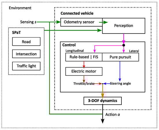
Figure 1. AV navigation block diagram. Sensor and SPaT data is represented by a green arrow, processed perception information in pink, longitudinal control in red, lateral control in blue, navigation inputs in orange and actions in black.

The proposed model uses a hierarchical approach (Figure 1). First, odometry data are retrieved by the internal sensors of the vehicle. It is assumed that the internal states of the vehicles are calculated through sensor fusion techniques and that proprioceptive data are always available and noise-free. Simultaneously, surrounding infrastructure provides SPaT data, which are assumed to be noise-free. Noisy measurements, data loss, and partial observations will be covered in future research. Then, perception module fuses the data to obtain pose information of the vehicle. Next, the pose is fed to the control module, which contains a rule-based or a FIS control systems for longitudinal actions and a pure pursuit controller for lateral actions. Finally, the control signals are sent to the three-degree-of-freedom (3-DOF) dynamics module of the CEV.

1.2. Contributions of This Paper

The major contributions of this paper are listed as follows:

1.

We demonstrate the feasibility of implementing rule- and a fuzzy inference system-based longitudinal navigation control systems on a pure electric platform. In both cases, power can be regenerated in the battery with appropriate design considerations. Previous efforts are mostly based on an internal combustion engine and hybrid vehicles, with little or no focus on electric power consumption and regeneration. These techniques are implemented for a B-class electric vehicle. The fuzzy inference system outperforms the rule-based strategy by a magnitude of two in terms of power regeneration. A benchmark experiment is performed in a crossroad intersection environment with a traffic light. Both strategies implement an eco-approach and departure strategy based on a coupled green light optimal speed advisory/regenerative braking system.

2.

Lateral, longitudinal, and rolling resistance forces are considered in the dynamic model. They directly impact on the navigation performance and power consumption and regeneration. Works on vehicle navigation usually rely on simplified kinematic models where no forces are considered. Longitudinal and lateral vehicle dynamics provide realistic behavior in terms of powertrain effort and vehicle motion. This differs from most state-of-the-art efforts, where dynamics are partially or totally neglected.

3.

A fully characterized electric machine that matches the vehicle powertrain is often neglected in the literature. Ideal actuators are a common choice. Efficiencies are assumed to be ideal or constant. From an energy standpoint, the vehicle propulsion electric motor is represented by its loss map. This allows computing a realistic bidirectional power demand and conversion efficiency.

In summary, the SPaT data usage, sensor fusion, longitudinal and lateral controllers, electric motor, and dynamic vehicle models add realism to the connected automated vehicle control system.

The paper is organized as follows: Section 2 presents the theoretical framework. The rule set and fuzzy inference system used for longitudinal control can be found in Section 3. Section 4 explains the rationale for the experiment design. It also contains the results of the experiment. Finally, Section 5 concludes this work and proposes future research directions. For notation clarity, a nomenclature list is provided at the end of this paper.

2. Powertrain Modeling

2.1. Vehicle Dynamic Model

The CEV is modeled as a 3-DOF bicycle model, as illustrated in Figure 2. Right and left wheels on the same axle are lumped into one element, both for the front and rear. The resulting rear wheel is fixed, whereas the front one can steer at an angle $\delta$. This angle is input for the vehicle dynamic model. The center of gravity C, mass m, polar moment of inertia $I_{zz}$ with respect to the z axis, and wheelbase L of the vehicle are constant parameters. The wheelbase is the distance between axles, thus $L=l_f+l_r$.

Figure 2. The 3-DOF bicycle CEV model.

The dynamic model of the vehicle is governed by the following equations:   

$$\begin{array}{cc}\hfill m\ddot{y}& =-m\dot{x}\dot{\psi }+F_{yf}+F_{yr}\hfill \end{array}$$

(1)

$$\begin{array}{cc}\hfill I_{zz}\ddot{\psi }& =l_f{F}_{yf}-l_r{F}_{yr}\hfill \end{array}$$

(2)

$$\begin{array}{cc}\hfill m\ddot{x}& =m\dot{y}\dot{\psi }+F_{xf}+F_{xr}\hfill \end{array}$$

(3)

These expressions show the coupled dynamic behavior between the longitudinal (x), lateral (y), and yaw ($\psi$) DOFs. The motion of the vehicle is mainly affected by the longitudinal force on the front (motoring) axle ($F_{xf}$). Moreover, external lateral forces on the front ($F_{yf}$) and rear ($F_{yr}$) axles are further contributions to vehicle dynamics. Roll, pitch, and vertical dynamics are assumed to be uncoupled from this representation. Aerodynamic contributions can be neglected even at the maximum speed of the class-B-sized vehicle ($14 \mathrm{m}/\mathrm{s}$). The longitudinal force components on the front axle is conformed by the powertrain propulsion minus the rolling resistance. On the rear axle, the longitudinal force is only given by the rolling resistance term:

$$\begin{array}{cc}\hfill F_{xf}& =\frac{T_m{\tau }_{gb}}{r_t}-\frac{F_c}{2}\mathrm{sign}\left(\dot{x}\right)\hfill \end{array}$$

(4)

$$\begin{array}{cc}\hfill F_{xr}& =-\frac{F_c}{2}\mathrm{sign}\left(\dot{x}\right)\hfill \end{array}$$

(5)

where $T_m$ is the electric motor torque, ${\tau }_{gb}$ the gear box gain, $r_t$ the tire radius, $\dot{x}$ the longitudinal speed of the vehicle, and $F_c$ the Coulomb friction. Aerodynamic effects are neglected in the longitudinal model due to the low velocity values expected in urban environments ($\dot{x}<60\mathrm{km}/\mathrm{h}$) [50]. The propulsion force is another input of the vehicle model. The cornering stiffness of the front and rear tires ($C_{\alpha f}$ and $C_{\alpha r}$) contribute to the lateral forces:

$$\begin{array}{cc}\hfill F_{yf}& =2C_{\alpha f}\left(\delta -{\theta }_{vf}\right)\hfill \end{array}$$

(6)

$$\begin{array}{cc}\hfill F_{yr}& =2C_{\alpha r}\left(-{\theta }_{vr}\right)\hfill \end{array}$$

(7)

In addition, tire velocity angles are given by

$$\begin{array}{cc}\hfill {\theta }_{vf}& =arctan\left(\frac{\dot{y}+l_f\dot{\psi }}{\dot{x}}\right)\hfill \end{array}$$

(8)

$$\begin{array}{cc}\hfill {\theta }_{vr}& =arctan\left(\frac{\dot{y}-l_r\dot{\psi }}{\dot{x}}\right)\hfill \end{array}$$

(9)

To favor faster computation, tire velocity angles were linearized assuming small angle deviations:

$$\begin{array}{cc}\hfill {\theta }_{vf}& \approx \frac{\dot{y}+l_f\dot{\psi }}{\dot{x}}\hfill \end{array}$$

(10)

$$\begin{array}{cc}\hfill {\theta }_{vr}& \approx \frac{\dot{y}-l_r\dot{\psi }}{\dot{x}}\hfill \end{array}$$

(11)

The nonlinear model in Equations (1)–(3) describe the lateral dynamics [51]. The global expressions are obtained by substituting Equations (10) into (6), and (11) into (7). Finally, resulting Equations (6) and (7) are substituted into (1) and (2) to yield the following expressions:

$$\begin{array}{cc}\hfill m\ddot{y}& =-m\dot{x}\dot{\psi }+2\left[C_{\alpha f}\left(\delta -\frac{\dot{y}+l_f\dot{\psi }}{\dot{x}}\right)+C_{\alpha r}\frac{l_r\dot{\psi }-\dot{y}}{\dot{x}}\right]\hfill \end{array}$$

(12)

$$\begin{array}{cc}\hfill I_{zz}\ddot{\psi }& =2\left[l_f{C}_{\alpha f}\left(\delta -\frac{\dot{y}+l_f\dot{\psi }}{\dot{x}}\right)-l_r{C}_{\alpha r}\frac{l_r\dot{\psi }-\dot{y}}{\dot{x}}\right]\hfill \end{array}$$

(13)

The parameters for the vehicle model used in this study were extracted from the vehicle templates in CarSIM^™ of a B-class hatchback vehicle in electric powertrain configuration, front-wheel drive. The values are listed in Table 2. The presented model is used to reproduce the dynamic behavior of the CEV in the rule-based and FIS GLOSA/RBS framework. This representation has been extensively used due its accurate vehicle dynamic behavior [52].

Table 2. B-class hatchback electric vehicle model parameters.

Parameter	Symbol	Value	Unit
Distance from COG to front axle	$l_f$	$1.04$	$\mathrm{m}$
Distance from COG to rear axle	$l_r$	$1.56$	$\mathrm{m}$
Mass	m	1377	$\mathrm{kg}$
Yaw polar moment of inertia	$I_{zz}$	$1343.1$	${\mathrm{kgm}}^2$
Front tire cornering stiffness	$C_{\alpha f}$	12	$\mathrm{kN}/\mathrm{rad}$
Rear tire cornering stiffness	$C_{\alpha r}$	11	$\mathrm{kN}/\mathrm{rad}$
Total rolling resistance force	$F_c$	5	$\mathrm{N}$

2.2. Motor Model

We use a look-up table containing the power losses of the machine for different torque and shaft speed combinations to describe the electric machine behavior. This approach is advantageous for the following reasons:

1.

The loss map gives means for a generic representation of the machine, which is able to fit any motor used in powertrain systems.

2.

Focus is given to conversion efficiency through motoring and regenerative quadrants.

3.

Power losses can be accurately characterized through electromagnetic finite-element models without the need to represent the machine through a lumped-parameter model.

4.

Electromagnetic dynamics are represented through a first-order low-pass filter with a time constant of 50 ms.

The electric machine loss map used in this case is illustrated in Figure 3.

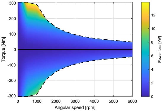
Figure 3. Electric machine loss map. Dashed lines represent the torque–speed characteristic limit. The solid line separates the motoring quadrant (positive torque) from the regenerative quadrant (negative torque).

Assuming perfect wheel rolling (no slip) and an ideally efficient gearbox, the powertrain mechanical power can be defined either through vehicle variables or through motor variables, i.e.,

$$P_m=F_{xf}\dot{x}-P_{rr}=T_m{\omega }_m-P_{rr}$$

(14)

where $T_m$ is the motor torque, ${\omega }_m$ is its angular speed, and $P_{rr}$ is the vehicle dissipated power due to rolling resistance.

During operation, the motor will attempt to impose a torque—positive or negative—on the vehicle based on the longitudinal control’s request. On the other hand, the vehicle will impose angular velocity on the motor shaft. Part of the mechanical power in Equation (14) will have an impact on the electrical domain of the motor, as it will drive the absorption or regeneration of electrical power, defined as:   

$$P_e=V_{dc}{i}_{dc}$$

(15)

with $V_{dc},i_{dc}$ being the voltage and current of the battery.

In motoring mode, the efficiency of the powertrain is defined as

$${\eta }_{mot}=\frac{P_m}{P_e}=\frac{P_m}{P_m+P_{loss}({\omega }_m,T_m)}$$

(16)

where $P_{loss}(·)$ represents the loss map function of the machine evaluated at a specific operating point.

Conversely, the powertrain has a regenerative efficiency given by

$${\eta }_{reg}=\frac{P_e}{P_m}=1-\frac{P_{loss}({\omega }_m,T_m)}{P_m}$$

(17)

Note that in any instance, a generic efficiency term must guarantee $\eta <1$.

3. Control Methods

This work proposes a hierarchical control system to optimize a CEV power consumption during EAD using GLOSA/RBS. Two strategies are presented to solve the longitudinal navigation problem: a rule-based and a FIS strategy. Both control methods retrieve information from the SPaT data and the vehicle location and current longitudinal speed. Then, a scenario is identified with the current status of the traffic light. The distance to the intersection and current longitudinal speed are used to determine a motor torque setpoint.

3.1. Rule-Based Controller

The rule-based motor torque setpoint generator is an empiric solution to the GLOSA/RBS problem. Initially, the SPaT data providing the traffic light status are retrieved from the surrounding infrastructure in the intersection. Then, the rule set is divided into three scenarios that depend on the status of the traffic light $\left(L_s\right)$: green, yellow, and red. Intersection-crossing or free-driving are the states that the CEV can be in. The selected motor torque $\left(\tau \right)$ ensures that the vehicle navigates in the environment without crossing the intersection during the red light. The navigation strategy can achieve power restoration by switching between motoring $(\tau >0)$, regenerative $(\tau <0)$, or neutral $(\tau =0)$ behavior of the motor while keeping the longitudinal speed $\left(\dot{x}\right)$ under the road’s speed limit $\left({\dot{x}}_{lim}\right)$ and maintaining comfort. In summary, the driving scenario that the CEV faces depends on $L_s$, $\dot{x}$ and the pose $\left(X\right)$ to produce a desired $\tau$. The algorithm for the rule-based controller is Algorithm 1.

Algorithm 1 Rule-based controller

Input:$X,\dot{x},L_s$ Output:$\tau$  if $L_s$ is green then      if $X\ge d_a$ then          if $\dot{x}\ge {\dot{x}}_{lim}$ then $\tau \leftarrow -{\tau }_{min}$          else if $\dot{x}<0$ then $\tau \leftarrow {\tau }_{min}$          else$\tau \leftarrow \frac{2}{3}{\tau }_{max}$          end if      else if $d_a<X<d_d$ then          if $\dot{x}\ge {\dot{x}}_{lim}$ then $\tau \leftarrow 0$          else if $0<\dot{x}<{\dot{x}}_{lim}$ then $\tau \leftarrow {\tau }_{max}$          else$\tau \leftarrow \frac{1}{2}{\tau }_{max}$          end if      else$\tau \leftarrow \frac{2}{3}{\tau }_{max}$      end if  else if $L_s$ is yellow then      if $X\ge d_a$ then          if $\dot{x}\ge {\dot{x}}_{slow}$ then $\tau \leftarrow -\frac{2}{3}{\tau }_{max}$          else if $0<\dot{x}<{\dot{x}}_{slow}$ then $\tau \leftarrow -{\tau }_{min}$          else$\tau \leftarrow {\tau }_{min}$          end if      else if $d_a<X<d_d$ then          if $\dot{x}\ge {\dot{x}}_{slow}$ then $\tau \leftarrow -\frac{5}{6}{\tau }_{max}$          else if $0<\dot{x}<{\dot{x}}_{slow}$ then $\tau \leftarrow -{\tau }_{min}$          else$\tau \leftarrow \frac{1}{6}{\tau }_{max}$          end if      else$\tau \leftarrow \frac{2}{3}{\tau }_{max}$      end if  else if $L_s$ is red then      if $X\ge d_a$ then          if $\dot{x}\ge {\dot{x}}_{slow}$ then $\tau \leftarrow -\frac{1}{4}{\tau }_{max}$          else if $\dot{x}\le 0$ then $\tau \leftarrow {\tau }_{min}$          else$\tau \leftarrow \frac{1}{10}{\tau }_{max}$          end if      else if $d_a<X<d_d$ then          if $\dot{x}\ge {\dot{x}}_{slow}$ then $\tau \leftarrow -{\tau }_{max}$          else if $0<\dot{x}<{\dot{x}}_{slow}$ then $\tau \leftarrow -{\tau }_{min}$          else$\tau \leftarrow \frac{1}{6}{\tau }_{max}$          end if      else$\tau \leftarrow \frac{2}{3}{\tau }_{max}$      end if  end if

3.1.1. Green Light

The road is divided into three segments: enter, approach, and departure zones. The first segment, enter, extends from the beginning of the road up to an approaching distance $\left(d_a\right)$. When the CEV is located in this area, it can have three behaviors. In the first case, the vehicle slowly increases its speed by applying a small torque ${\tau }_{min}$ if the speed is in the $0<\dot{x}<{\dot{x}}_{lim}$ interval, where ${\dot{x}}_{lim}$ is the speed limit of the road. In the second case, if the speed limit is surpassed, a small negative torque $-{\tau }_{min}$ is used to decrease the velocity. This event encourages power regeneration. Negative speeds are avoided by applying a $\frac{2}{3}{\tau }_{max}$ torque. The third case avoids using negative values for $\dot{x}$. The second road segment, approach, is defined in the $d_a<d<d_d$ interval, where $d_d$ is the beginning of the departing zone or the point after the traffic light in the intersection. As this segment is very close to the crossroad, the CEV will focus on crossing the intersection and reaching the departing zone by applying a ${\tau }_{max}$ torque. Navigating to a higher speed than the limit is avoided by applying a null torque. Negative speeds are avoided by applying a $\frac{1}{2}{\tau }_{max}$ torque. In the final road segment, departure, the vehicle is allowed to increase its throttle by $\frac{2}{3}{\tau }_{max}$ to cross the intersection and continue navigating.

3.1.2. Yellow Light

The general goal of the navigation strategy during a yellow light is to reduce speed to avoid crossing the intersection during the red light and applying aggressive braking maneuvers. There are three different behaviors in the enter interval. The first is to slowly reduce the longitudinal speed of the CEV by applying a $-{\tau }_{min}$ torque if the current velocity is in the $0<\dot{x}<{\dot{x}}_{slow}$ range, where ${\dot{x}}_{slow}$ is the minimum speed in which the CEV can navigate on the road. If the vehicle is navigating faster than ${\dot{x}}_{slow}$, a $-\frac{2}{3}{\tau }_{max}$ torque is applied. Negative speeds are avoided by applying a ${\tau }_{min}$. The approach segment implements similar behaviors to those in the enter segment. The main difference are that a $-\frac{5}{6}{\tau }_{max}$ braking torque that is applied for speeds greater than ${\dot{x}}_{slow}$, and a $\frac{1}{6}{\tau }_{max}$ is applied to avoid negative speeds. The vehicle is allowed to increase its throttle by $\frac{2}{3}{\tau }_{max}$ after crossing the intersection in the departure zone. The staged braking strategy during this traffic light status induces a regenerative state for CEV navigation.

3.1.3. Red Light

The strategy of the rule-based control system is to avoid braking to a full stop during red lights at road intersections. The CEV faces a scenario of maximum power regeneration after the speed has been reduced during the yellow light strategy. If the CEV is in the first navigational stage, any longitudinal speed greater than ${\dot{x}}_{slow}$ causes a $-\frac{1}{4}{\tau }_{max}$ throttle. A $\frac{1}{10}{\tau }_{max}$ throttle is applied to keep the vehicle moving in the $0<\dot{x}<{\dot{x}}_{slow}$ interval. A full stop and negative velocities are avoided by applying a ${\tau }_{min}$ torque. The approach road interval strategy applies a ${\tau }_{max}$ maneuver for speeds greater than ${\dot{x}}_{slow}$. A $-{\tau }_{min}$ torque is used to reduce speeds in the range $0<\dot{x}<{\dot{x}}_{slow}$. Full stop and negative speeds are avoided with a $\frac{1}{6}{\tau }_{max}$. The vehicle increases its throttle torque to $\frac{2}{3}{\tau }_{max}$ once it is in the departure zone.

3.2. Fuzzy Inference System

Fuzzy set theory is used to specify how a crisp measurement fits into a linguistic description. It is considered a generalization of classic set theory, as it represents uncertainty and memberships. Fuzzy logic maps a degree of membership of a system to a fuzzy set using classic Boolean logic. However, it resembles human-like reasoning with the usage of linguistic variables and decision-making processes with uncertainty [53]. FISs rely on a previously defined knowledge base coming from an expert. They evaluate a statement that relates an antecedent with an implication. These types of systems can represent mathematical complex systems with a simple set of rules model with fuzzy sets [54].

Longitudinal control with FIS require the previous design and validation of appropriate membership functions (MFs). Related research has proposed the usage of uniformly distributed triangular MFs to model the normalized error as input and identical triangular functions with shoulder functions for the brake/throttle as output [55]. However, an uneven distribution and form of MF is proposed to model inter-vehicle distance and the speed error [56]. Similarly, a set with a high number of unevenly distributed MFs was used to capture the behavior of the longitudinal model of a vehicle in [57]. Those guidelines provided insight on how to design the longitudinal FIS-based controller. Three FIS were deigned, one for each state of the traffic light. The green light FIS uses the simplest set of MFs and rules. The yellow FIS and red FIS have a greater number of linguistic variables for the inputs. Even and uneven distributions for the MFs were used to better represent the behavior of every physical variable.

The following MFs are used to represent the physical variables involved in the longitudinal navigation control system: $\dot{x}$, $\left(X\right)$, and $\tau$. $L_s$ is not fuzzified, as the light status is a Boolean value. Inputs $\dot{x}$ and X are modeled with Gaussian, Gaussian combination, S, and Z MFs. The longitudinal speed of the CEV is normalized to a $[-1,1]$ interval. Long-term motor braking can cause reverse motion in the vehicle. Hence, positive and negative values are considered. The maximum speed ${\dot{x}}_{max}$ of the 3-DOF model is not reachable in urban environments. Thus, the speed limit of the road is used as higher and lower boundaries with an $\epsilon$ tolerance such that

$${\dot{x}}_{norm}=\frac{\dot{x}}{(1+\epsilon ){\dot{x}}_{lim}}$$

(18)

The relative location $\left(X_r\right)$ of the CEV respect the intersection $\left(X_I\right)$ is also normalized in a $[-1,1]$ range. The normalization distance of the location is either the SPaT converage $\left(d_{SPaT}\right)$ range or the maximum distance in which a visual sensor can detect the traffic light status $\left(d_{sensor}\right)$.

$$X_r=\frac{X_I-X}{\max (d_{SPaT},d_{sensor})}$$

(19)

The output $\tau$ uses triangular, linear S, and Z MFs. The maximum motor torque ${\tau }_{max}$ is used to normalize $\tau$ in a $[-1,1]$ interval. Defuzzification is performed using the Mamdani method.

$${\tau }_{norm}=\frac{\tau }{{\tau }_{max}}$$

(20)

Three different FISs are used to generate the desired longitudinal behavior of the CEV, one for each of the traffic $L_s$: green, yellow, and red. A multiplexer selects the appropriate system according to the data provided by SPaT.

3.2.1. Green Light

The location $X_r$ of the CEV is represented as three linguistic variables: entering, approaching, and departing (Figure 4a). Entering is a Z-shaped MF that covers from the beginning of the road up to a fifth of the road before the intersection. Approaching is represented as a two-sided Gaussian MF that runs from $0.4$ to a value slightly greater than zero. Finally, Departing uses a S-shaped MF that starts a road length before the intersection and ends with the road. Four variables model the velocity ${\dot{x}}_{norm}$ of the CEV: reverse, slow, normal, and fast (Figure 4b). Reverse is a Z-shaped MF that goes from the negative speed limit up to zero in an open interval. Slow uses a Gaussian MF representation centered at a tenth of ${\dot{x}}_{norm}$. A normal generalized bell-shaped MF describes speeds that are greater than slow and less than the speed limit. Any velocity that is near or greater than the speed limit is part of the S-shaped MF fast. The motor torque ${\tau }_{norm}$ is described as three variables: reverse, neutral, and forward (Figure 4c). Reverse covers all negative torques up to zero. A steep linear Z-shaped MF is employed to express this variable. An unbalanced triangular MF centered on zero depicts the neutral torque. The negative part of the MF has a pronounced slope, while the positive ends in a fifth. This behavior was chosen to promote null or slow positive torque. The forward variable is a S-shaped MF with slow growth starting from zero.

Figure 4. Green light fuzzy sets.

A set of five rules models the desired behavior during the navigation with $L_s=\mathrm{green}$ (Algorithm 2). The main goal is to take advantage of the current status of the light and navigate toward the intersection in the smallest amount of time. Special conditions are considered to avoid navigating backwards or surpassing the speed limit of the road.

Algorithm 2 Green light FIS knowledge base

Input:  $X_r,{\dot{x}}_{norm}$ Output:  $\_norm$  if $X_r\to$ entering $\&{\dot{x}}_{norm}\to$ fast then      ${\tau }_{norm}\leftarrow \mathrm{reverse}$  else if $X_r\to$ entering $\&{\dot{x}}_{norm}\to \neg$ fast then      ${\tau }_{norm}\leftarrow \mathrm{forward}$  else if $X_r\to$ approaching $\&{\dot{x}}_{norm}\to$ fast then      ${\tau }_{norm}\leftarrow \mathrm{reverse}$  else if $X_r\to$ approaching $\&{\dot{x}}_{norm}\to \neg$ fast then      ${\tau }_{norm}\leftarrow \mathrm{forward}$  else if $X_r\to$ departing then      ${\tau }_{norm}\leftarrow \mathrm{forward}$  end if

3.2.2. Yellow Light

The same three linguistic variables employed for the $X_r$ set in the green light are used for the yellow light: entering, approaching, and departing (Figure 5a). No changes are made on the type of MF for each variable. However, their limits are changed. The entering zone is reduced to a half of its original size. On the other hand, the approaching zone is extended three times. Similarly, all the variables of ${\dot{x}}_{norm}$ in the green light set are reused (Figure 5b). The limits and properties of the slow, normal, and fast MF are updated. Slow and normal MFs are narrowed and displaced to the left without touching a zero value. Fast is just shifted to the left. Reverse remains unchanged. The three original MFs of ${\tau }_{norm}$ are preserved. Neutral and forward continue as they were originally defined. Reverse is shifted to the left. A new triangular MF with symmetric boundaries is introduced to add a soft reverse variable. This new MF is designed to perform braking and regenerative actions for the CEV.

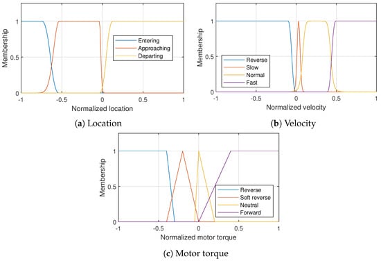
Figure 5. Yellow fuzzy sets.

Nine rules describe the designed navigation navigation behavior for $L_s=\mathrm{yellow}$ (Algorithm 3). The main goal is to greatly reduce the speed of the CEV according to its pose and velocity without reaching a full stop, as a part of the RB/EAD strategy. During this maneuver, power can be regenerated because of the performance the electric motor. Crossing the intersection during the yellow light should be avoided. However, traversing the crossroad is encouraged if the speed is high and safety constraints are compromised. Reverse and over the speed limit navigation situations are avoided through specific rules.

Algorithm 3 Yellow light FIS knowledge base

Input:  $X_r,{\dot{x}}_{norm}$ Output:  ${\tau }_{norm}$  if $X_r\to$ entering $\&{\dot{x}}_{norm}\to$ reverse then      ${\tau }_{norm}\leftarrow \mathrm{forward}$  else if $X_r\to$ entering $\&{\dot{x}}_{norm}\to$ slow then      ${\tau }_{norm}\leftarrow \mathrm{neutral}$  else if $X_r\to$ entering $\&{\dot{x}}_{norm}\to$ normal then      ${\tau }_{norm}\leftarrow$ soft reverse  else if $X_r\to$ entering $\&{\dot{x}}_{norm}\to$ fast then      ${\tau }_{norm}\leftarrow \mathrm{reverse}$  else if $X_r\to$ approaching $\&{\dot{x}}_{norm}\to$ reverse then      ${\tau }_{norm}\leftarrow \mathrm{forward}$  else if $X_r\to$ approaching $\&{\dot{x}}_{norm}\to$ slow then      ${\tau }_{norm}\leftarrow \mathrm{neutral}$  else if $X_r\to$ approaching $\&{\dot{x}}_{norm}\to$ normal then      ${\tau }_{norm}\leftarrow$ soft reverse  else if $X_r\to$ approaching $\&{\dot{x}}_{norm}\to$ fast then      ${\tau }_{norm}\leftarrow \mathrm{reverse}$  else if $X_r\to$ departing then      ${\tau }_{norm}\leftarrow \mathrm{forward}$  end if

3.2.3. Red Light

The $X_r$ and ${\dot{x}}_{norm}$ fuzzy sets for the $L_s=\mathrm{red}$ are identical to the ones presented in $L_s=\mathrm{yellow}$ (Figure 5a,b). The same criteria are considered to fuzzify both crisp values and require no additional modification. Nonetheless, an extra linguistic variable $softforward$ is added to ${\tau }_{norm}$ (Figure 6). The full throttle is not needed during $L_s=\mathrm{red}$ in entering or approaching zones. Therefore, this rule is needed for smoothly navigating toward the intersection. Additionally, it is easier for the motor to switch to neutral or soft reverse. The forward rule is shifted to the right without further modification.

Figure 6. Red light fuzzy sets.

A nine-rule knowledge base is used for $L_s=\mathrm{red}$ (Algorithm 4). The goal of this system it to navigating toward the intersection while regenerating the most amount of power. Constantly reducing the speed to a minimum without reaching full stop guarantees the complement of RB/EAD. This strategy is valid for the entering and approaching zones. During the entering stage, the speed is slowly reduced. In contrast, the braking rate is increased in the approaching zone to avoid crossing the intersection. Specific rules are designed to evade reverse navigation because of the motor regenerative behavior.

Algorithm 4 Red light FIS knowledge base

Input:  $X_r,{\dot{x}}_{norm}$ Output:  ${\tau }_{norm}$  if $X_r\to$ entering $\&{\dot{x}}_{norm}\to$ reverse then      ${\tau }_{norm}\leftarrow \mathrm{forward}$  else if $X_r\to$ entering $\&{\dot{x}}_{norm}\to$ slow then      ${\tau }_{norm}\leftarrow$ soft forward  else if $X_r\to$ entering $\&{\dot{x}}_{norm}\to$ normal then      ${\tau }_{norm}\leftarrow$ neutral  else if $X_r\to$ entering $\&{\dot{x}}_{norm}\to$ fast then      ${\tau }_{norm}\leftarrow$ soft reverse  else if $X_r\to$ approaching $\&{\dot{x}}_{norm}\to$ reverse then      ${\tau }_{norm}\leftarrow \mathrm{forward}$  else if $X_r\to$ approaching $\&{\dot{x}}_{norm}\to$ slow then      ${\tau }_{norm}\leftarrow \mathrm{neutral}$  else if $X_r\to$ approaching $\&{\dot{x}}_{norm}\to$ normal then      ${\tau }_{norm}\leftarrow$ soft reverse  else if $X_r\to$ approaching $\&{\dot{x}}_{norm}\to$ fast then      ${\tau }_{norm}\leftarrow \mathrm{reverse}$  else if $X_r\to$ departing then      ${\tau }_{norm}\leftarrow \mathrm{forward}$  end if

4. Experiments

4.1. Experiment Design

It is assumed that the CEV can retrieve information from the environment with SPaT data or can obtain the status of the traffic light of the intersection with a visual sensor. The internal states are obtained through an odometer. The vehicle uses said data to compute a motor torque setpoint for a longitudinal navigation strategy to achieve RB/EAD. Two strategies were developed: a rule- and a FIS-based strategy. The torque goes into an electric motor, the powertrain, and finally into the 3-DOF vehicle.

4.2. Environment

The street layout is a right-hand, three-lane, one-direction, and no-slope crossroad with a main and secondary roads (Figure 7). Both roads are 300 $\mathrm{m}$ long and intersect at the middle. The lanes are 4 $\mathrm{m}$ wide. The boundaries of the roads are delimited by solid white lines. A traffic light is located at the middle of the crossroad. Crosswalks are available at the road intersection. It is assumed that the whole environment has SPaT data access without communication interruptions or data integrity threats. The CEV is meant to navigate in a straight path from its initial pose $X_i$ to the goal pose $X_f$. The initial conditions of the CEV, traffic light, and simulation parameters are shown in Table 3.

Figure 7. Road layout.

Table 3. Environment parameters.

Parameter	Notation	Default Setting
Initial pose $\left[\mathrm{m}\right]$	$X_i=[x_i,y_i]$	$[0,0]$
Initial steering angle $\left[\mathrm{rad}\right]$	$\delta$	0
Initial velocity $[\mathrm{m}/\mathrm{s}]$	$\dot{X_i}=[{\dot{x}}_i,{\dot{y}}_i]$	min: $[0,0]$
		max: $[13,0]$
Goal pose $\left[\mathrm{m}\right]$	$X_f=[x_f,y_f]$	$[300,0]$
Green light duration $\left[\mathrm{s}\right]$	$t_{Lg}$	16
Yellow light duration $\left[\mathrm{s}\right]$	$t_{Ly}$	4
Red light duration $\left[\mathrm{s}\right]$	$t_{Lr}$	20
Initial light	$L_s$	$L_s\in [t_{Lg},t_{Ly},t_{Lr}]$
Vehicle sample time $\left[\mathrm{s}\right]$	$t_s$	0.001
Rules and FIS sample time $\left[\mathrm{s}\right]$	$t_{Ds}$	0.1

4.3. Integrated Longitudinal Navigation

Algorithm 5 depicts the integrated longitudinal control system for the implementation of GLOSA/RBS/EAD. The results of said algorithm are presented in terms of navigation success rate and power regeneration. Both generated control methods are based on empiric and expert knowledge. A fixed-step solver was selected with different sampling times for the physical elements $\left(t_s\right)$ and the control methods $\left(t_{Ds}\right)$ (Table 3). The rule- and FIS-based controllers were tested and validated in a variety of initial speeds and initial light status time. The complete performance data of the rule- and FIS-based longitudinal navigation systems can be found in Table 4.

Table 4. Navigation system performance.

Method	Velocity	Acceleration	Completion Time	Success Rate
	[m/s]	[m/s2]	[s]	[%]
Rule-based	min: 0.025	min: −3.02	33.32	96.43
	max: 22.46	max: 3.01
	avg: 12.22	avg: 0.28
FIS-based	min: 0.092	min: −4.51	27.76	95.9
	max: 23.83	max: 3.74
	avg: 13.08	avg: 0.39

The rule-based system successfully completed $96.43\%$ of the tests. The cases in which the intersection was not successfully crossed were due to extreme situation such as the following: The vehicle was traveling at very high speeds at the approaching zone of the intersection and the status of traffic light was green. Then, there was not enough road to decrease the longitudinal speed and make a stop during the sequence change to yellow and red. The fuzzy system had a similar success rate to the rule-based, $95.9\%$. The performance in terms of speed and acceleration of both control systems is comparable. Likewise, navigation complies with comfort as the acceleration never surpasses the $[-9.6,4.905]\mathrm{m}/{\mathrm{s}}^2$ interval. Completion time is consistent with the the longitudinal velocity and throttle.

Algorithm 5 Integrated data acquisition and control algorithm for the connected electric vehicle

1: Initialize the control methods mentioned in Section 3 2: Define ego vehicle and environment 3: Start V2X communication 4: for  $t=0,1,2,\cdots ,T$do 5:     Retrieve SPaT data 6:     Retrieve pose data 7:     if navigation = rules then 8:         Compute selected ${\tau }_{norm}$ 9:     else if navigation = FIS then 10:         Compute $X_r$ and ${\dot{x}}_{norm}$ 11:         Fuzzify crisp values 12:         Use knowledge base according to $L_s$ 13:         Defuzzify linguistic value 14:         Compute selected ${\tau }_{norm}$ 15:     end if 16:     Apply a ${\tau }_{max}$ gain 17:     Input the $\tau$ setpoint to the electric motor 18:     Apply the motor torque to the vehicle powertrain 19: end for

Three samples of the performed tests on rule- and FIS-based controllers are presented: one for $L_s=\mathrm{green}$ with starting time $t=0$ s and initial speed ${\dot{x}}_i=0$ m/s (Figure 8), another one for $L_s=\mathrm{yellow}$ with starting time $t=0$ s and initial speed ${\dot{x}}_i=5$ m/s (Figure 9), and, finally, for $L_s=\mathrm{red}$ with starting time $t=15$ s and initial speed ${\dot{x}}_i=11$ m/s (Figure 10). The samples are evaluated with the pose X and velocity $\dot{x}$ metrics. The pose plot depicts the world-based road in meters for x against time. It also shows the position of the intersection and the current status $L_s$ of the traffic light. The velocity plot illustrates the velocity behavior of the CEV through time. Each test is described in the next paragraphs.

Figure 8. Performance metrics for test 1.

Figure 9. Performance metrics for test 2.

Figure 10. Performance metrics for test 3.

4.3.1. Test 1: Green Light Starting From Rest

It can be noted from Figure 8a how the rule- and FIS-based systems approach the intersection and successfully cross during $L_s=\mathrm{green}$ before its change to its next state. From Figure 8b, it can be seen how the vehicle starts with an initial velocity of ${\dot{x}}_i=0$ m/s. The rule-based system increases its speed until $t\approx 7$ s. Then, it adopts a CC strategy with small increments of speed to navigate the approach zone. Speed is kept constant for an interval of ∼10 s. After the junction is passed, the vehicle increments its speed. The FIS-based controller adopts a more aggressive strategy as it constantly increments its speed until $t\approx$10 s. Finally, it navigates at a constant speed for ∼3 s until overtaking the crossroad and increments its speed.

4.3.2. Test 2: Yellow Light Starting from a Slow Speed

Figure 9a shows how both longitudinal control systems approach the intersection and successfully cross during $L_s=\mathrm{green}$. In both cases, the CEV adopts an RBS/EAD strategy to avoid crossing during the $L_s=\mathrm{yellow}$ or $L_s=\mathrm{red}$ status. The vehicle starts with an initial velocity of ${\dot{x}}_i=5$ m/s (Figure 9b). The rule-based system initially decreases its speed. Then, a CC behavior is used for $t\approx$ 22 s. This approach is maintained until the CEV detects a change of $L_s$ to $\mathrm{green}$. Then, after the junction is passed, the vehicle increments its speed. The FIS-based controller adopts a different strategy. Initially, it increments its speed. Then, when the approach zone is reached it decreases its speed until it is close do zero. When $L_s=\mathrm{green}$, it constantly increments its speed, crosses the intersection, and continues on its path.

4.3.3. Test 3: Red Light Starting from a High Speed

Both longitudinal control systems approach the intersection and successfully cross during $L_s=\mathrm{green}$ (Figure 10a). The CEV adotps an RBS/EAD strategy to avoid crossing during the $L_s=\mathrm{red}$ status. The vehicle starts with an initial velocity of ${\dot{x}}_i=11$ m/s (Figure 10b). The rule-based system initially decreases its speed to $v\approx$ 7 m/s. Then, the CEV detects a change of $L_s$ to $\mathrm{green}$. The vehicle gradually increments its speed during the approach phase. Small CC behaviors are adopted during this stage. When it crosses the intersection, it increases its speed to continue navigating. The FIS-based controller adopts a less conservative strategy. First, it applies CC until the light change. Next, it increments its speed, goes across the intersection, and continues on its path.

4.4. Power Consumption and Regeneration

Related work has focused on pure ICEV or hybrid vehicles. They measure the performance of their EAD systems based on fuel savings and time to completion. We are proposing techniques for CEV. Thus, the power efficiency of the rule- and FIS-based systems is an additional metric used to evaluate the performance of the proposed EAD controllers. The following parameters have been chosen to provide better insight: average power $\left(\overline{P}\right)$, braking/motoring power ratio $\left({\overline{P}}_r\right)$, and the motoring $\left({\eta }_{mot}\right)$ and regenerative $\left({\eta }_{reg}\right)$ efficiencies.

The average power is an algebraic mean of the instantaneous power P in a time t. The constant sampling time $t_s$ (Table 3) allows this computation to be valid.

$$\overline{P}=\frac{1}{T}\sum _{t=0}^T{P}_t$$

(21)

The regeneration/motoring power ratio provides information on how many instants of the drive cycle were destined to reduce or increment the speed of the CEV and how much power could be restored.

$${\overline{P}}_r=\frac{{\overline{P}}_{brake}}{{\overline{P}}_{mot}}$$

(22)

Power consumption and restoration depend on the initial conditions of the tests and the rationale used to design the longitudinal control system. The performance of the rule- and FIS-based systems can be found in Table 5 and Table 6, respectively. They relate the initial conditions of $L_s$, $t_i$, and ${\dot{x}}_i$ with the mechanical and electrical average motoring $\left({\overline{P}}_{mot}\right)$ and regeneration $\left({\overline{P}}_{reg}\right)$ power with their corresponding ${\overline{P}}_r$ and their efficiencies ${\eta }_{reg}$ and ${\eta }_{mot}$.

Table 5. Rule-based controller power performance.

${\mathit{L}}_{\mathit{s}}$ Time Interval $\left[\mathbf{s}\right]$	${\dot{\mathit{x}}}_{\mathit{i}}$ Interval $[\mathbf{m}/\mathbf{s}]$		Mechanical			Electrical		${\mathit{\eta }}_{\mathit{mot}}$ [%]	${\mathit{\eta }}_{\mathit{reg}}$ [%]
		${\overline{\mathit{P}}}_{\mathit{mot}}$  $\left[\mathbf{kW}\right]$	${\overline{\mathit{P}}}_{\mathit{reg}}$  $\left[\mathbf{kW}\right]$	${\overline{\mathit{P}}}_{\mathit{r}}$ [%]	${\overline{\mathit{P}}}_{\mathit{mot}}$  $\left[\mathbf{kW}\right]$	${\overline{\mathit{P}}}_{\mathit{reg}}$  $\left[\mathbf{kW}\right]$	${\overline{\mathit{P}}}_{\mathit{r}}$ [%]
	$[0,5)$	21.66	6.38	29.36	26.92	4.91	18.12	80.44	77.05
$(0,10)$	$[5,10)$	22.54	5.46	24.25	27.32	4.21	15.24	82.50	77.03
	$[10,13]$	21.57	4.68	21.68	25.58	3.62	13.95	84.31	77.44
	$[0,5)$	15.79	3.00	18.99	19.76	2.23	11.28	79.90	74.60
$[10,16]$	$[5,10)$	19.35	4.60	24.16	24.22	3.48	14.55	79.89	75.55
	$[10,13]$	19.92	5.36	27.87	24.90	4.11	17.14	80.01	76.65
	$[0,5)$	10.62	0.33	3.19	12.86	0.25	1.99	82.57	75.99
$(16,20]$	$[5,10)$	15.32	2.69	17.50	18.57	2.03	10.86	82.51	75.55
	$[10,13]$	19.21	5.79	30.95	23.69	4.68	20.24	81.08	80.80
	$[0,5)$	11.99	0.53	4.44	14.51	0.42	2.89	82.58	78.80
$(20,30]$	$[5,10)$	18.88	3.03	15.76	22.87	2.48	10.65	82.57	81.90
	$[10,13]$	24.46	6.50	26.54	30.01	5.49	18.28	81.50	84.45
	$(0,5)$	15.11	0.82	5.44	18.31	0.64	3.49	82.51	77.76
$(30,40]$	$[5,10)$	23.32	3.82	16.17	28.11	3.14	11.02	82.98	82.18
	$[10,13]$	26.12	7.39	27.96	31.04	6.35	20.22	84.14	85.94
Average		19.06	4.02	19.61	23.24	3.20	12.66	81.96	78.78

Table 6. Fuzzy logic-based controller power performance.

${\mathit{L}}_{\mathit{s}}$ Time Interval $\left[\mathbf{s}\right]$	${\dot{\mathit{x}}}_{\mathit{i}}$ Interval $[\mathbf{m}/\mathbf{s}]$		Mechanical			Electrical		${\mathit{\eta }}_{\mathit{mot}}$ [%]	${\mathit{\eta }}_{\mathit{reg}}$ [%]
		${\overline{\mathit{P}}}_{\mathit{mot}}$  $\left[\mathbf{kW}\right]$	${\overline{\mathit{P}}}_{\mathit{reg}}$  $\left[\mathbf{kW}\right]$	${\overline{\mathit{P}}}_{\mathit{r}}$ [%]	${\overline{\mathit{P}}}_{\mathit{mot}}$  $\left[\mathbf{kW}\right]$	${\overline{\mathit{P}}}_{\mathit{reg}}$  $\left[\mathbf{kW}\right]$	${\overline{\mathit{P}}}_{\mathit{r}}$ [%]
	$[0,5)$	21.48	12.78	59.13	25.76	10.61	40.35	83.38	83.04
$(0,10)$	$[5,10)$	23.96	9.78	37.77	28.15	8.23	26.90	85.10	84.15
	$[10,13]$	21.69	6.26	26.58	25.10	5.29	19.32	86.43	84.54
	$[0,5)$	16.10	5.19	34.47	19.51	3.97	21.68	82.53	76.55
$[10,16]$	$[5,10)$	16.74	10.35	61.85	20.22	8.14	40.03	82.79	78.72
	$[10,13]$	18.27	17.21	90.77	21.88	13.86	60.57	83.48	80.55
	$[0,5)$	15.04	5.02	33.39	18.03	3.65	20.25	83.43	72.71
$(16,20]$	$[5,10)$	15.02	6.66	44.29	17.97	4.97	27.65	83.60	74.65
	$[10,13]$	14.94	8.68	58.38	17.90	6.65	37.35	83.45	76.65
	$[0,5)$	17.20	8.20	47.36	20.52	6.07	29.36	83.80	74.01
$(20,30]$	$[5,10)$	18.38	8.91	48.36	21.98	6.59	29.89	83.61	73.91
	$[10,13]$	19.82	8.08	41.23	23.77	6.13	26.08	83.35	75.97
	$[0,5)$	19.38	2.03	10.34	22.28	1.59	6.89	84.85	78.16
$(30,40]$	$[5,10)$	21.42	6.96	32.29	25.04	5.42	21.39	85.56	77.91
	$[10,13]$	23.79	7.27	30.20	27.82	5.85	20.65	85.52	80.52
Average		18.88	8.22	43.76	22.39	6.46	28.55	84.05	78.13

The rule-based longitudinal system has consistent performance when it enters the intersection at the beginning of the green light $t=(0,10],L_s\in \mathrm{green}$. Regardless of the initial speed, the ${\overline{P}}_{mot}$ of the system is consistent in both mechanical and electrical systems. On the other hand, ${\overline{P}}_{reg}$ decreases uniformly as the speed increases because of the adopted strategy of crossing the junction as soon as possible. It can be noted that ${\eta }_{mot}$ increases linearly with ${\dot{x}}_i$, whereas ${\eta }_{reg}$ remains constant. A similar behavior can be found in the FIS-based system. However, ${\overline{P}}_r$ is almost doubled at low speeds, increased by a half on medium speeds and greater than $15\%$ at high speeds when compared with the rule-based performance. The motoring and regeneration efficiencies show an almost identical operation to the ones in the other system but with higher values.

For $t=[10,16],L_s\in \mathrm{green}$ segment or late green at the traffic light, there is constant power consumption at medium and high initial speeds and lower power consumption for slow speed in the rule-based system. That behavior is found to be inverse for the FIS. Slow and medium speeds show the constant and higher use of power for high velocity. Regeneration of power proportional to ${\dot{x}}_i$ can be spotted in both controllers. The FIS regenerates from two to three times the power of the rule-based system. Up to $60\%$ of the consumed electrical power can be restored by the CEV. The ${\eta }_{mot}$ value is almost constant in both systems, with higher efficiency in the FIS, while ${\eta }_{reg}$ increases in both cases, with better power usage for the FIS.

A new behavior is found during the yellow light or $t=(16,20],L_s\in \mathrm{yellow}$ for the rule-based system. Power consumption and regeneration increase linearly with ${\dot{x}}_i$. Immediate CC navigation causes a very small ${\overline{P}}_r$ for low speeds. On the other hand, medium and high speeds require an initial brake to avoid crossing the intersection during $L_s=\mathrm{red}$ and encourage CC. This implies an increasing ${\overline{P}}_r$. The FIS controller has a constant power consumption, but a growing regeneration rate as in the rule-based system. ${\overline{P}}_r$ is ten times greater during slow, more than double for medium, and almost double for high ${\dot{x}}_i$. The motoring efficiency is kept constant for each system with a higher value for the FIS. The efficiency for regeneration power is consistent for low and medium speeds and greater for high speeds for the rule-based system, whereas the FIS continuously increases.

The rule-based system has a continuously increasing power consumption and regeneration during the initial red light phase or $t=(20,30],L_s\in \mathrm{red}$. Slow initial speeds cause little regeneration due to CC as in $L_s\in \mathrm{yellow}$. Similarly, the faster the vehicle starts navigating, the greater a negative throttle should be applied to start CC, causing the increment of ${\overline{P}}_r$ from below $5\%$ to above one-fifth of the electric motoring power. The FIS power consumption increments slowly, but the regeneration is almost constant. This implies a ${\overline{P}}_r$ of almost one-third of the consumed electric power. The value of ${\eta }_{mot}$ is very near in the rule- and FIS controllers, whereas there is a higher efficiency in ${\eta }_{reg}$ of the rule-based system.

Finally, the rule-based controller exhibits a similar behavior to the previous stage for the late red light or $t=(30,40],L_s\in \mathrm{red}$. This applies to ${\overline{P}}_r$, ${\eta }_{mot}$ and ${\eta }_{reg}$. The FIS has a different performance. This time, its power consumption as well as the regeneration increment slowly. However, a small reduction in the restored power can be noted at high speeds. Motoring and regeneration efficiencies are higher when compared with the previous stage but smaller than for the rule-based ones.

The difference in the success rate of both navigation systems is not significant. Both are close to $96\%$. The average mechanical motoring power of the rule-based controller and the FIS is almost identical. The rule-based employs slightly more power. Nonetheless, the power regeneration and ratio performance of both systems exhibit different behaviors. The FIS regenerated electrical power outperforms the one of the rule-based by $101.96\%$. Consequently, the regeneration/motoring power ratio is $125.55\%$ higher.

5. Conclusions and Future Research

In this work, two longitudinal navigational strategies were developed for implementing RBS on EAD while navigating signalized intersections with a traffic light. In the virtual environment, internal data are acquired through odometry and external data through SPaT coming from V2X communications. The data are fed into a perception module that provides location information to a CEV controller. The controller implements a lateral pure pursuit algorithm. A rule- or FIS-based longitudinal controller determines the setpoint for an electric motor that outputs a torque that is implemented by the powertrain. Said torque is then transformed into positive or negative throttle. Finally, it is applied into a dynamic model of an ego vehicle. This model provides a realistic representation of the plant. The proposed algorithms implement a longitudinal navigation strategy that account for speed limit compliance, comfort, and power efficiency and regeneration. The numerical results enable the possibility of implementation of both systems into a physical system for controlled tests.

Navigation of CEV at urban intersections with power management and restoration is a field with open research opportunities. After simulation, the numerical results show that the proposed systems can be employed as a benchmark for future researchers to validate new systems in terms of SPaT data, longitudinal velocity and acceleration, comfort, time to completion, success rate, consumed and regenerated power, and motoring and regeneration efficiency. Therefore, the open research questions along these lines are:

1.

Multiple intersection environments to alter the state of charge of a battery during sustained navigation.

2.

Background vehicles to increase the complexity of the problem and help better understand the safety, comfort, and power management challenges.

3.

The use of machine learning, artificial intelligence, or predictive control techniques that use the proposed longitudinal navigation systems as a benchmark and design rationale.

4.

Enhancing vehicles with visual and inertial sensors to cover non-SPaT areas. Sensor fusion techniques are required to tackle data availability, thereby expanding the problem into a partially observable Markov decision process.

5.

The integration of the proposed approach within more complex energy management and control strategies, where multiple vehicle functionalities and behaviors coexist.

6.

Safe and eco-approach and departure navigation in highly dynamic situations, such as lane changing, merging, overtaking, or obstacle avoidance maneuvers.

References

- United-Nations. The Sustainable Development Goals Report; UN: New York, NY, USA, 2022.
- Sudhakar, S.; Sze, V.; Karaman, S. Data Centers on Wheels: Emissions From Computing Onboard Autonomous Vehicles. IEEE Micro 2023, 43, 29–39. [Google Scholar] [CrossRef]
- Mo, Z.; Shi, R.; Di, X. A physics-informed deep learning paradigm for car-following models. Transp. Res. Part C Emerg. Technol. 2021, 130, 103240. [Google Scholar] [CrossRef]
- Ruan, K.; Zhang, J.; Di, X.; Bareinboim, E. Causal Imitation Learning via Inverse Reinforcement Learning. In Proceedings of the Eleventh International Conference on Learning Representations, Kigali, Rwanda, 1–5 May 2023. [Google Scholar]
- Ruan, K.; Di, X. Learning Human Driving Behaviors with Sequential Causal Imitation Learning. In Proceedings of the AAAI Conference on Artificial Intelligence, Virtual, 22 February–1 March 2022; Volume 36, pp. 4583–4592. [Google Scholar] [CrossRef]
- International-Energy-Agency. Clean Energy Innovation; International-Energy-Agency: Paris, France, 2020.
- Chen, G.; Wang, F.; Li, W.; Hong, L.; Conradt, J.; Chen, J.; Zhang, Z.; Lu, Y.; Knoll, A. NeuroIV: Neuromorphic Vision Meets Intelligent Vehicle Towards Safe Driving with a New Database and Baseline Evaluations. IEEE Trans. Intell. Transp. Syst. 2022, 23, 1171–1183. [Google Scholar] [CrossRef]
- Yeong, D.J.; Velasco-Hernandez, G.; Barry, J.; Walsh, J. Sensor and Sensor Fusion Technology in Autonomous Vehicles: A Review. Sensors 2021, 21, 2140. [Google Scholar] [CrossRef] [PubMed]
- Woo, A.; Fidan, B.; Melek, W.W. Localization for Autonomous Driving. In Handbook of Position Location; Wiley: Hoboken, NJ, USA, 2019; pp. 1051–1087. [Google Scholar] [CrossRef]
- Giacalone, J.P.; Bourgeois, L.; Ancora, A. Challenges in aggregation of heterogeneous sensors for Autonomous Driving Systems. In Proceedings of the 2019 IEEE Sensors Applications Symposium (SAS), Sophia Antipolis, France, 11–13 March 2019. [Google Scholar] [CrossRef]
- Kim, T.; Park, T.H. Extended Kalman Filter (EKF) Design for Vehicle Position Tracking Using Reliability Function of Radar and Lidar. Sensors 2020, 20, 4126. [Google Scholar] [CrossRef] [PubMed]
- Claussmann, L.; Revilloud, M.; Gruyer, D.; Glaser, S. A Review of Motion Planning for Highway Autonomous Driving. IEEE Trans. Intell. Transp. Syst. 2020, 21, 1826–1848. [Google Scholar] [CrossRef]
- Liu, W.; Hua, M.; Deng, Z.; Huang, Y.; Hu, C.; Song, S.; Gao, L.; Liu, C.; Xiong, L.; Xia, X. A Systematic Survey of Control Techniques and Applications: From Autonomous Vehicles to Connected and Automated Vehicles. arXiv 2023. [Google Scholar] [CrossRef]
- Montanaro, U.; Dixit, S.; Fallah, S.; Dianati, M.; Stevens, A.; Oxtoby, D.; Mouzakitis, A. Towards connected autonomous driving: Review of use-cases. Veh. Syst. Dyn. 2018, 57, 779–814. [Google Scholar] [CrossRef]
- Guanetti, J.; Kim, Y.; Borrelli, F. Control of connected and automated vehicles: State of the art and future challenges. Annu. Rev. Control 2018, 45, 18–40. [Google Scholar] [CrossRef]
- Guan, J.; Chen, G.; Huang, J.; Li, Z.; Xiong, L.; Hou, J.; Knoll, A. A Discrete Soft Actor-Critic Decision-Making Strategy with Sample Filter for Freeway Autonomous Driving. IEEE Trans. Veh. Technol. 2023, 72, 2593–2598. [Google Scholar] [CrossRef]
- Wang, Z.; Han, K.; Tiwari, P. Digital Twin-Assisted Cooperative Driving at Non-Signalized Intersections. IEEE Trans. Intell. Veh. 2022, 7, 198–209. [Google Scholar] [CrossRef]
- Williams, N.; Wu, G.; Closas, P. Impact of positioning uncertainty on eco-approach and departure of connected and automated vehicles. In Proceedings of the 2018 IEEE/ION Position, Location and Navigation Symposium (PLANS), Monterey, CA, USA, 23–26 April 2018. [Google Scholar] [CrossRef]
- Altan, O.D.; Wu, G.; Barth, M.J.; Boriboonsomsin, K.; Stark, J.A. GlidePath: Eco-Friendly Automated Approach and Departure at Signalized Intersections. IEEE Trans. Intell. Veh. 2017, 2, 266–277. [Google Scholar] [CrossRef]
- Hao, P.; Wu, G.; Boriboonsomsin, K.; Barth, M.J. Eco-Approach and Departure (EAD) Application for Actuated Signals in Real-World Traffic. IEEE Trans. Intell. Transp. Syst. 2019, 20, 30–40. [Google Scholar] [CrossRef]
- Committee, V.C.T. V2X Communications Message Set Dictionary; SAE International: Warrenda, PA, USA, 2020. [Google Scholar] [CrossRef]
- Wágner, T.; Ormándi, T.; Tettamanti, T.; Varga, I. SPaT/MAP V2X communication between traffic light and vehicles and a realization with digital twin. Comput. Electr. Eng. 2023, 106, 108560. [Google Scholar] [CrossRef]
- Jin, K.; Li, X.; Wang, W.; Hua, X.; Long, W. Energy-optimal speed control for connected electric buses considering passenger load. J. Clean. Prod. 2023, 385, 135773. [Google Scholar] [CrossRef]
- Wang, Z.; Wu, G.; Barth, M.J. Cooperative Eco-Driving at Signalized Intersections in a Partially Connected and Automated Vehicle Environment. IEEE Trans. Intell. Transp. Syst. 2020, 21, 2029–2038. [Google Scholar] [CrossRef]
- Ye, F.; Hao, P.; Qi, X.; Wu, G.; Boriboonsomsin, K.; Barth, M.J. Prediction-Based Eco-Approach and Departure at Signalized Intersections with Speed Forecasting on Preceding Vehicles. IEEE Trans. Intell. Transp. Syst. 2019, 20, 1378–1389. [Google Scholar] [CrossRef]
- Dong, H.; Zhuang, W.; Chen, B.; Yin, G.; Wang, Y. Enhanced Eco-Approach Control of Connected Electric Vehicles at Signalized Intersection with Queue Discharge Prediction. IEEE Trans. Veh. Technol. 2021, 70, 5457–5469. [Google Scholar] [CrossRef]
- Wu, G.; Hao, P.; Wang, Z.; Jiang, Y.; Boriboonsomsin, K.; Barth, M.; McConnell, M.; Qiang, S.; Stark, J. Eco-Approach and Departure along Signalized Corridors Considering Powertrain Characteristics. SAE Int. J. Sustain. Transp. Energy Environ. Policy 2021, 2, 1–16. [Google Scholar] [CrossRef]
- Jia, Y.; Luo, G.; Zhang, Y. Development of optimal speed trajectory control strategy for electric vehicles to suppress battery aging. Green Energy Intell. Transp. 2022, 1, 100030. [Google Scholar] [CrossRef]
- Wang, Q.; Dong, H.; Ju, F.; Zhuang, W.; Lv, C.; Wang, L.; Song, Z. Adaptive Leading Cruise Control in Mixed Traffic Considering Human Behavioral Diversity. arXiv 2022. [Google Scholar] [CrossRef]
- Dong, H.; Zhuang, W.; Ding, H.; Zhou, Q.; Wang, Y.; Xu, L.; Yin, G. Event-driven Energy-efficient Driving Control in Urban Traffic for Connected Electric Vehicles. IEEE Trans. Transp. Electrif. 2022, 9, 99–113. [Google Scholar] [CrossRef]
- Mei, P.; Karimi, H.R.; Yang, S.; Xu, B.; Huang, C. An adaptive fuzzy sliding-mode control for regenerative braking system of electric vehicles. Int. J. Adapt. Control Signal Process. 2021, 36, 391–410. [Google Scholar] [CrossRef]
- Saiteja, P.; Ashok, B.; Wagh, A.S.; Farrag, M.E. Critical review on optimal regenerative braking control system architecture, calibration parameters and development challenges for EVs. Int. J. Energy Res. 2022, 46, 20146–20179. [Google Scholar] [CrossRef]
- Mello, E.F.; Bauer, P.H. Energy-Optimal Speed Trajectories between Stops. IEEE Trans. Intell. Transp. Syst. 2020, 21, 4328–4337. [Google Scholar] [CrossRef]
- Li, N.; Yang, J.; Jiang, J.; Hong, F.; Liu, Y.; Ning, X. Study on Speed Planning of Signalized Intersections with Autonomous Vehicles Considering Regenerative Braking. Processes 2022, 10, 1414. [Google Scholar] [CrossRef]
- Qian, G.; Fu, T.; Sun, L. Research on the fuel consumption conservation potential of ADAS on passenger cars. E3S Web Conf. 2021, 268, 01035. [Google Scholar] [CrossRef]
- Simchon, L.; Rabinovici, R. Real-Time Implementation of Green Light Optimal Speed Advisory for Electric Vehicles. Vehicles 2020, 2, 35–54. [Google Scholar] [CrossRef]
- Yan, Y.; Han, D.; Shen, T.; Wang, Z.; Wang, J.; Yin, G. Velocity Trajectory Planning of Electric Vehicles with Consideration of the Passenger’s Individual Preferences. In Proceedings of the 2022 6th CAA International Conference on Vehicular Control and Intelligence (CVCI), Nanjing, China, 28–30 October 2022. [Google Scholar] [CrossRef]
- Jiang, X.; Zhang, J.; Wang, B. Energy-Efficient Driving for Adaptive Traffic Signal Control Environment via Explainable Reinforcement Learning. Appl. Sci. 2022, 12, 5380. [Google Scholar] [CrossRef]
- Claussmann, L.; Revilloud, M.; Glaser, S.; Gruyer, D. A study on al-based approaches for high-level decision making in highway autonomous driving. In Proceedings of the 2017 IEEE International Conference on Systems, Man, and Cybernetics (SMC), Banff, AB, Canada, 5–8 October 2017. [Google Scholar] [CrossRef]
- Grosan, C.; Abraham, A. Rule-Based Expert Systems. In Intelligent Systems Reference Library; Springer: Berlin/Heidelberg, Germany, 2011; pp. 149–185. [Google Scholar] [CrossRef]
- Li, N.; Chen, H.; Kolmanovsky, I.; Girard, A. An Explicit Decision Tree Approach for Automated Driving. In Volume 1: Aerospace Applications. Advances in Control Design Methods, Bio Engineering Applications, Advances in Non-Linear Control, Adaptive and Intelligent Systems Control, Advances in Wind Energy Systems, Advances in Robotics, Assistive and Rehabilitation Robotics, Biomedical and Neural Systems Modeling, Diagnostics, and Control, Bio-Mechatronics and Physical Human Robot, Advanced Driver Assistance Systems and Autonomous Vehicles, Automotive Systems; American Society of Mechanical Engineers: Tysons, VA, USA, 2017. [Google Scholar] [CrossRef]
- Magdalena, L. Fuzzy Rule-Based Systems. In Springer Handbook of Computational Intelligence; Springer: Berlin/Heidelberg, Germany, 2015; pp. 203–218. [Google Scholar] [CrossRef]
- Guo, J.; Li, W.; Wang, J.; Luo, Y.; Li, K. Safe and Energy-Efficient Car-Following Control Strategy for Intelligent Electric Vehicles Considering Regenerative Braking. IEEE Trans. Intell. Transp. Syst. 2022, 23, 7070–7081. [Google Scholar] [CrossRef]
- Wang, Z.; Wu, G.; Scora, G. MOVESTAR: An Open-Source Vehicle Fuel and Emission Model based on USEPA MOVES. arXiv 2020. [Google Scholar] [CrossRef]
- An, F.; Barth, M.; Norbeck, J.; Ross, M. Development of Comprehensive Modal Emissions Model: Operating Under Hot-Stabilized Conditions. Transp. Res. Rec. J. Transp. Res. Board 1997, 1587, 52–62. [Google Scholar] [CrossRef]
- Hao, P.; Boriboonsomsin, K.; Wang, C.; Wu, G.; Barth, M. Connected Eco-approach and Departure System for Diesel Trucks. SAE Int. J. Commer. Veh. 2021, 14, 217–227. [Google Scholar] [CrossRef] [PubMed]
- Oswald, D.; Hao, P.; Williams, N.; Barth, M. Development of an Innovation Corridor Testbed for Shared Electric Connected and Automated Transportation. In A Research Reportfrom the National Center for Sustainable Transportation; National Center for Sustainable Transportation: Davis, CA, USA, 2021. [Google Scholar] [CrossRef]
- Han, J.; Karbowski, D.; Rousseau, A. State-Constrained Optimal Solutions for Safe Eco-Approach and Departure at Signalized Intersections. In Proceedings of the ASME 2020 Dynamic Systems and Control Conference, Virtual, 5–7 October 2020; American Society of Mechanical Engineers: New York, NY, USA, 2020. [Google Scholar] [CrossRef]
- Coulter, R.C. Implementation of the Pure Pursuit Path Tracking Algorithm; Technical Report CMU-RI-TR-92-01; Carnegie Mellon University: Pittsburgh, PA, USA, 1992. [Google Scholar]
- Genta, G.; Morello, L. The Automotive Chassis: Volume 2: System Design; Mechanical Engineering Series; Springer International Publishing: Cham, Switzerland, 2020. [Google Scholar]
- Jazar, R.N. Vehicle Dynamics: Theory and Application; Springer: New York, NY, USA, 2008. [Google Scholar] [CrossRef]
- Miloradović, D.; Glisovic, J.; Stojanovic, N.; Grujic, I. Simulation of vehicle’s lateral dynamics using nonlinear model with real inputs. In Proceedings of the IOP Conference Series: Materials Science and Engineering, Kazimierz Dolny, Poland, 21–23 November 2019; IOP Publishing: Bristol, UK, 2019; Volume 659, p. 012060. [Google Scholar] [CrossRef]
- Zadeh, L. Fuzzy sets. Inf. Control 1965, 8, 338–353. [Google Scholar] [CrossRef]
- Ponce-Cruz, P.; Ramirez-Figueroa, F.D. Intelligent Control Systems with LabVIEW™; Springer: London, UK, 2010. [Google Scholar] [CrossRef]
- Cabello, F.; Acuna, A.; Vallejos, P.; Orchard, M.E.; del Solar, J.R. Design and validation of a fuzzy longitudinal controller based on a vehicle dynamic simulator. In Proceedings of the 2011 9th IEEE International Conference on Control and Automation (ICCA), Santiago, Chile, 19–21 December 2011. [Google Scholar] [CrossRef]
- Mattas, K.; Botzoris, G.; Papadopoulos, B. Safety aware fuzzy longitudinal controller for automated vehicles. J. Traffic Transp. Eng. (Engl. Ed.) 2021, 8, 568–581. [Google Scholar] [CrossRef]
- Baz, R.; Majdoub, K.E.; Giri, F.; Taouni, A. Self-tuning fuzzy PID speed controller for quarter electric vehicle driven by In-wheel BLDC motor and Pacejka’s tire model. IFAC-PapersOnLine 2022, 55, 598–603. [Google Scholar] [CrossRef]
Disclaimer/Publisher’s Note: The statements, opinions and data contained in all publications are solely those of the individual author(s) and contributor(s) and not of MDPI and/or the editor(s). MDPI and/or the editor(s) disclaim responsibility for any injury to people or property resulting from any ideas, methods, instructions or products referred to in the content. |
© 2023 by the authors. Licensee MDPI, Basel, Switzerland. This article is an open access article distributed under the terms and conditions of the Creative Commons Attribution (CC BY) license (https://creativecommons.org/licenses/by/4.0/).