A Time-Series Model for Varying Worker Ability in Heterogeneous Distributed Computing Systems

Abstract

In this paper, we consider the problem of estimating the time-dependent ability of workers participating in distributed matrix-vector multiplication over heterogeneous clusters. Specifically, we model the workers’ ability as a latent variable and introduce a log-normally distributed working rate as a function of the latent variable with parameters so that the working rate increases as the latent ability of workers increases, and takes positive values only. This modeling is motivated by the need to reflect the impact of time-dependent external factors on the workers’ performance. We estimate the latent variable and parameters using the expectation-maximization (EM) algorithm combined with the particle method. The proposed estimation and inference on the working rates are used to allocate tasks to the workers to reduce expected latency. From simulations, we observe that our estimation and inference on the working rates are effective in reducing expected latency.

1. Introduction

In order to meet the ever-growing demand for massive-scale computations using a large amount of data, distributed computing systems have become a central part of many machine learning algorithms [1]. However, distributed computing systems often face the problem of waiting for slow workers, called stragglers [2]. To overcome this issue and provide straggler tolerance, Lee et al. introduced redundancy to distributed matrix multiplication [3]. Specifically, the authors show that computational latency can be reduced using the $(n,k)$ maximum distance separable (MDS) code, since collecting any $k(<n)$ out of n workers’ results would complete the assigned task.

Including the idea proposed by Lee et al. [3], there has been a growing body of work using coding to mitigate the straggler problem in homogeneous clusters. This includes coding for high-dimensional matrix multiplication [4,5], matrix multiplication that considers the architecture of practical systems [6], gradient descent [7,8,9], convolution [10], and non-linear computation using a learning-based approach [11]. Mitigating the effects of stragglers is not limited to environments that consider computing clusters but can also be used in many types of distributed computing architectures that may struggle with stragglers or failures. Examples include fog computing, computation with a deadline, mobile edge computing, layered architecture of edge-assisted Internet of Things, and federated learning [10,12,13].

The system designs under homogeneous assumptions in potentially heterogeneous clusters can significantly reduce the overall performance [14]. For example, suppose that we assign the same amount of tasks to two workers with different computing capabilities. Consider a time for two workers to finish the tasks. A worker with relatively large computing capabilities takes less time to complete the given task than a worker with relatively small computing capabilities, on average. Thus, the expected time to complete the entire task is highly dependent on the time for a worker with relatively small computing capabilities to finish the task. In other words, the uniform load allocation to workers without considering the heterogeneous characteristics of the workers’ computing capabilities can lead to the performance degradation of computing systems. Reflecting on these points, research has been conducted under the assumption of heterogeneous clusters [15,16]. In [15], the authors present an asymptotically optimal load allocation to minimize the expected task completion delay for fully heterogeneous clusters. Similarly, in [16], an optimal load allocation is proposed to minimize the expected execution time under the assumption of group heterogeneity, which means that workers in different groups have different latency statistics.

In this work, we consider a scenario where the ability of each heterogeneous worker changes over time. While the work of [15,16] covers distributed computation in a heterogeneous environment, the authors assume that each worker’s ability is a fixed known constant. However, in reality, even workers designed to maintain a constant level of ability can have time-dependent abilities due to external factors such as changes in temperature and humidity over time [17]. If we do not estimate workers’ abilities, the basic load allocation method would be the uniform load allocation, which assigns the same amount of tasks to each worker. However, as we mentioned earlier, this load allocation method can potentially lead to a loss of system performance. Thus, the estimation of workers’ abilities is essential to improve system latency.

We model the aggregated impact of such factors on the worker’s ability as a normal distribution and set the worker’s ability as a latent variable. As demonstrated in several prior works [3,4,6,15,16], it is widely accepted that the runtime of a worker is often modeled by an exponential distribution. We define the working rate of a worker as the rate of the exponentially distributed runtime and assume that the working rate is log-normally distributed with two parameters: the mean and standard deviation of the logarithm of the working rate, respectively. The log-normal distribution is a good fit for the working rate since it ensures that the working rate takes only positive values and increases as the latent ability of a worker increases. We aim to estimate the latent variable and parameters associated with the ability/working rate of the worker so that one can properly allocate the workload on the workers in distributed computing. Many pieces of research have been devoted to the analysis of the time-series data with latent variables from different points of view [18,19,20,21]. In this paper, we employ particle methods to deal with both the estimation of parameters and the inference of latent variables.

Contribution: The key contributions of this work are summarized as follows.

• To the best of our knowledge, we first model the workers’ ability that changes over time with latent variables.
• We present an estimation algorithm for the parameters and latent variables of the workers’ ability using the expectation maximization (EM) algorithm combined with the particle method.
• We verify the validity of the presented algorithm with Monte Carlo simulations.
• We confirm the validity of our inference by verifying that the load allocation based on the estimated workers’ ability achieves the lower bound of the expected execution time.

2. Preliminaries

In this section, we describe our system model and model assumptions. Then an optimal load allocation is introduced according to the system model and the model assumptions.

2.1. System Model

We focus on the distributed matrix-vector multiplication over a master–worker setup in time-dependent heterogeneous clusters (described in Figure 1). At time t, we assign a task to compute the multiplication of ${\mathit{A}}_t$ and ${\mathbf{b}}_t$ to the N distributed workers with different runtimes for a given matrix ${\mathit{A}}_t\in {\mathbb{R}}^{k\times d}$ and the input vector ${\mathbf{b}}_t\in {\mathbb{R}}^{d\times 1}$. We assume that N workers are divided into G groups. Each group has a different number of workers and a different working rate. The workers in each group have the same working rate. We denote the number of workers in group i as $N_i$, which implies that

$$\sum _{i\in \left[G\right]}{N}_i=N.$$

The tasks are successively assigned to the workers at time points $t=t_0,t_1,\dots t_T,t_{T+1},\dots$. To demonstrate our computation model, we present the uncoded and coded computations for a given task computing the multiplication of ${\mathit{A}}_t$ and ${\mathbf{b}}_t$ assigned at time t as follows.

Figure 1. Illustration of the time-dependent heterogeneous cluster (task assigned at time t). The master sends the input vector ${\mathbf{b}}_t$ to the N workers, each of which stores ${\mathit{A}}_{i,j,t}$ and ${\tilde{\mathit{A}}}_{i,j,t}$ in uncoded and coded computations, respectively, for $i\in \left[G\right]$ and $j\in \left[N_i\right]$; (a) worker j in group i computes the multiplication of ${\mathit{A}}_{i,j,t}$ and ${\mathbf{b}}_t$ with the working rate ${\mu }_{i,t}$, and sends back the computation results to the master; (b) worker j in group i computes the multiplication of ${\tilde{\mathit{A}}}_{i,j,t}$ and ${\mathbf{b}}_t$ with the working rate ${\mu }_{i,t}$, and sends back the results to the master.

2.1.1. Uncoded Computation

The rows of ${\mathit{A}}_t$ are divided into G disjoint submatrices as

$${\mathit{A}}_t=[{\mathit{A}}_{1,t};{\mathit{A}}_{2,t};\dots ;{\mathit{A}}_{G,t}]$$

where

$${\mathit{A}}_{i,t}=[{\mathit{A}}_{i,1,t};{\mathit{A}}_{i,2,t};\dots ;{\mathit{A}}_{i,N_i,t}]\in {\mathbb{R}}^{N_i{l}_{i,t}\times d}$$

and

$$\sum _{i\in \left[G\right]}{N}_i{l}_{i,t}=k.$$

Here, ${\mathit{A}}_{i,j,t}\in {\mathbb{R}}^{l_{i,t}\times d}$ is a submatrix of ${\mathit{A}}_{i,t}$ allocated to worker j in group i for $i\in \left[G\right]$ and $j\in \left[N_i\right]$. Worker j in group i is assigned a subtask to compute the multiplication of ${\mathit{A}}_{i,j,t}$ and ${\mathbf{b}}_t$ after receiving the input vector ${\mathbf{b}}_t$ from the master. Then, worker j in group i computes the multiplication of ${\mathit{A}}_{i,j,t}$ and ${\mathbf{b}}_t$ and sends back the result to the master. After the master collects the computation results from all the workers, the desired computation result ${\mathit{A}}_t{\mathbf{b}}_t$ can be obtained.

2.1.2. Coded Computation

We apply an $(n,k)$ MDS code to the rows of ${\mathit{A}}_t$ to obtain the coded matrix $\widetilde{{\mathit{A}}_t}\in {\mathbb{R}}^{n\times d}$. Afterward, the rows of ${\tilde{\mathit{A}}}_t$ are grouped into N submatrices as

$${\tilde{\mathit{A}}}_t=[{\tilde{\mathit{A}}}_{1,t};{\tilde{\mathit{A}}}_{2,t};\dots ;{\tilde{\mathit{A}}}_{G,t}],$$

where

$${\tilde{\mathit{A}}}_{i,t}=[{\tilde{\mathit{A}}}_{i,1,t},{\tilde{\mathit{A}}}_{i,2,t},\dots ,{\tilde{\mathit{A}}}_{i,N_i,t}]\in {\mathbb{R}}^{N_i{l}_{i,t}\times d}$$

is the coded data matrix allocated to the workers in group i and

$$\sum _{i\in \left[G\right]}{N}_i{l}_{i,t}=n.$$

Here, worker j in group i is assigned a subtask to compute the multiplication of ${\tilde{\mathit{A}}}_{i,j,t}\in {\mathbb{R}}^{l_{i,t}\times d}$ and ${\mathbf{b}}_t$ for $i\in \left[G\right]$ and $j\in \left[N_i\right]$. Worker j in group i sends the computation result ${\tilde{\mathit{A}}}_{i,j,t}{\mathbf{b}}_t$ to the master after finishing the subtask multiplying ${\tilde{\mathit{A}}}_{i,j,t}$ and ${\mathbf{b}}_t$. The master can retrieve the desired computation result ${\mathit{A}}_t{\mathbf{b}}_t$ by combining the inner products of any $k(<n)$ coded rows with ${\mathbf{b}}_t$ from the MDS property.

For efficient load allocation to the distributed workers, we need to estimate the workers’ ability, which is assumed to change over time. To do so, for the first T time points $t=t_0,t_1,\dots ,t_T$, we assign the matrix-vector multiplication tasks using the uncoded computation framework to measure the runtime of all the workers. Here, every worker is assigned the same amount of the subtask, i.e., we set $l_{i,t}=k/N$ for $i\in \left[G\right]$, $j\in \left[N_i\right]$, and $t=t_0,t_1,\dots ,t_T$. Based on the observations on the runtime, we estimate the parameters and latent variables of the working rates. Afterward ($t>t_T$), the coded computation is applied using the load allocation $l_{i,t}$ based on the estimated working rates. The latent variable is obtained continuously for each time step to properly allocate $l_{i,t}$ to the workers. The detailed process of estimating the working rates will be shown in Section 3.

2.2. Model Assumptions

For the task assigned at time t, we assume the time taken for calculating an inner product of a row of ${\mathit{A}}_{i,t}$; the input vector ${\mathbf{b}}_t$ follows the shifted exponential distribution with rate ${\mu }_{i,t}$, which is defined as the working rate of workers in group i. It is assumed that workers having the same working rate form a group. In other words, workers in a group have the same computing capabilities.

We model the working rate ${\mu }_{i,t}$ as

$${\mu }_{i,t}:=e^{X_{i,t}}$$

(1)

using a latent variable $X_{i,t}.$ Here, $X_{i,t}$ denotes the ability of workers in group i for a subtask assigned at time t.

For workers in group i, it is assumed that the zero state $X_{i,0}$ follows the normal distribution $\mathcal{N}(m,{\sigma }^2)$, where m and $\sigma$ are model parameters. Let us denote $\mathbf{\theta }=(m,\sigma )$. We write $f_0$ as the probability density function of $x_{i,0}$ given parameters,

$$f_0\left(x_{i,0}\right|\mathbf{\theta }=(m,\sigma ))=\frac{1}{\sqrt{2\pi }\sigma }{e}^{-\frac{1}{2{\sigma }^2}{\left(x_{i,0}-m\right)}^2}.$$

(2)

The ability of workers may vary over time, which is formulated by

$$X_{i,t}:=X_{i,t-1}+{ϵ}_{i,t},$$

where ${ϵ}_{i,t}$ is a white noise that is independent across group i and time t and follows the normal distribution with zero mean and variance ${\sigma }_{ϵ}^2$. Here, ${ϵ}_{i,t}$ represents the change in the worker ability as the time elapses from $t-1$ to t. In this work, we assume ${\sigma }_{ϵ}$ is given. For a precise formulation, we denote the distribution of $X_{i,t}$ given $X_{i,t-1}=x_{i,t-1}$ by

$$f\left(x_{i,t}\right|x_{i,t-1})=\frac{1}{\sqrt{2\pi }{\sigma }_{ϵ}}{e}^{-\frac{1}{2{\sigma }_{ϵ}^2}{\left(x_{i,t}-x_{i,t-1}\right)}^2},$$

(3)

which is the probability density function of the normal distribution with mean $x_{i,t-1}$ and variance ${\sigma }_{ϵ}^2$.

We assume that $t_{j+1}-t_j$ is a sufficient time interval for the workers to carry out their subtasks allocated at time $t_j$. We further assume that a task is assigned at successive time points spaced at uniform intervals, i.e., $t_{j+1}-t_j=t_{l+1}-t_l$ for all $j\ne l$. Then, $t_0,t_1,\dots ,t_T$ can be rewritten as $0,1,\dots ,T$ for notational convenience.

Let ${\eta }_{i,j,t}$ be the observed variable that indicates the runtime of worker $j\in \left[N_i\right]$ in group $i\in \left[G\right]$ for a given data matrix

$${\mathit{A}}_{i,j,t}\in {\mathbb{R}}^{l_{i,t}\times d}$$

with the following probability density function:

$$p\left({\eta }_{i,j,t}\right|X_{i,t},l_{i,t})=\frac{{\mu }_{i,t}}{l_{i,t}}{e}^{-\frac{{\mu }_{i,t}}{l_{i,t}}({\eta }_{i,j,t}-l_{i,t})}.$$

(4)

Since ${\eta }_{i,j,t}$’s are independent, we obtain the probability density function g of the observation ${\eta }_{i,t}$ given by

$$g\left({\eta }_{i,t}\right|x_{i,t},l_{i,t})=\prod _{t\in {\left[T\right]}_0}\prod _{j\in \left[N_i\right]}g\left({\eta }_{i,j,t}\right|x_{i,t},l_{i,t}).$$

(5)

for $i\in \left[G\right]$, $j\in \left[N_i\right]$, and $t\in {\left[T\right]}_0$. It follows from (5) that we have the probability density function of ${\eta }_{i,0:T}$ (observations for workers in group i through the time points $t\in {\left[T\right]}_0$) as follows:

$$p\left({\eta }_{i,0:T}\right|x_{i,0:T},l_{i,0:T})=\prod _{t\in {\left[T\right]}_0}g\left({\eta }_{i,t}\right|x_{i,t},l_{i,t}),$$

where $l_{i,0:T}$ and $x_{i,0:T}$ denote the number of rows of the data matrix assigned to workers in group i and the ability of workers in group i at time $t\in {\left[T\right]}_0$, respectively. Then, for all of the workers,

$$\begin{array}{c}\hfill p\left({\eta }_{1:G,0:T}\right|x_{1:G,0:T},l_{1:G,0:T})=\prod _{i\in \left[G\right]}\prod _{t\in {\left[T\right]}_0}g\left({\eta }_{i,t}\right|x_{i,t},l_{i,t})\\ \hfill =\prod _{i\in \left[G\right]}p\left({\eta }_{i,0:T}\right|x_{i,0:T},l_{i,0:T}),\end{array}$$

where ${\eta }_{1:G,0:T}$, $x_{1:G,0:T}$, and $l_{1:G,0:T}$ represent the overall observations, the workers’ ability, and the number of rows of the assigned matrices for workers in group $i\in \left[G\right]$ at time $t\in {\left[T\right]}_0$, respectively.

2.3. Optimal Load Allocation

In this subsection, we provide an analysis of load allocation given ${\widehat{\mu }}_{i,t}$, for $i\in \left[G\right]$ at time t. The previous work [16] presents the optimal load allocation to minimize the expected task runtime. We reproduce the results in [16] with some definitions according to our system model.

Let ${\mathcal{T}}_i$ denote the task runtime taken to calculate the inner product of $l_{i,t}$ rows of ${\tilde{\mathit{A}}}_{i,t}$ with ${\mathbf{b}}_t$ at a worker in group i at time t. We assume that ${\mathcal{T}}_i$s are independent random variables, with the shifted exponential distribution as follows

$$F_i\left[\eta \right]=Pr[{\mathcal{T}}_i\le \eta ]=1-e^{-\frac{{\mu }_{i,t}}{l_{i,t}}\left(\eta -l_{i,t}\right)}$$

(6)

for $i\in \left[G\right]$ and $\eta \ge l_{i,t}$. Here, it is assumed that the cumulative distribution function of the task runtime for a worker in group i to calculate one inner product is

$$1-e^{{\mu }_{i,t}(\eta -1)}$$

for $\eta \ge 1.$

Let ${\mathcal{T}}_{r_{i,t}:N_i}^{l_{i,t}}$ denote the $r_{i,t}$-th order statistics of $N_i$ random variables following the distribution in (6). We define

$$\mathcal{T}=\underset{i\in \left[G\right]}{max}\left\{{\mathcal{T}}_{r_{i,t}:N_i}^{l_{i,t}}\right\}$$

(7)

as the task runtime for the master to finish the given task.

Theorem 1

(Theorem 2 in [16]). The optimal load allocation $(l_{1,t}^{*},l_{2,t}^{*},\dots ,l_{G,t}^{*})$ to achieve the minimum of

$$\underset{i\in \left[G\right]}{max}\left\{\mathrm{E}\left[{\mathcal{T}}_{r_{i,t}:N_i}^{l_{i,t}}\right]\right\},$$

denoted by ${\mathcal{T}}^{★}$, is determined as follows:

$$l_{i,t}^{*}=\frac{k}{r_{i,t}^{*}+{\sum }_{i^{\prime }(\ne i)\in \left[G\right]}{r}_{i^{\prime },t}^{*}\frac{\xi (r_{i,t}^{*},N_i)}{\xi \left(r_{i^{\prime },t}^{*},N_{i^{\prime }}\right)}}$$

(8)

for $i\in \left[G\right]$, where

$$\begin{array}{c}\hfill r_{i,t}^{*}=N_i\left(1+\frac{1}{W_{-1}\left(-e^{-\left({\mu }_{i,t}+1\right)}\right)}\right),\end{array}$$

$$\begin{array}{cc}\hfill & \xi (r_{i,t}^{*},N_i)=1+\frac{1}{{\mu }_{i,t}}log\left(-W_{-1}\left(-e^{-({\mu }_{i,t}+1)}\right)\right),\hfill \end{array}$$

and

$$\frac{r_{i,t}^{*}}{\xi \left(r_{i,t}^{*},N_i\right)}=-\frac{{\mu }_{i,t}{N}_i}{W_{-1}(-e^{-({\mu }_{i,t}+1)})}.$$

Here, $W_{-1}\left(x\right)$ is the lower branch of the Lambert W function. ($W_{-1}\left(x\right)$ denotes the branch satisfying $W\left(x\right)e^{W\left(x\right)}=x$ and $W\left(x\right)\le -1$). Then the minimum expected execution time, ${\mathcal{T}}^{★}$, is represented as

$$-\frac{k}{{\sum }_{j\in \left[G\right]}\frac{{\mu }_{i,t}{N}_i}{W_{-1}\left(-e^{-\left({\mu }_{i,t}+1\right)}\right)}}.$$

Then, we have

$$\mathrm{E}\left[\mathcal{T}\right]\ge \underset{i\in \left[G\right]}{max}\left\{\mathrm{E}\left[{\mathcal{T}}_{r_{i,t}:N_i}^{l_{i,t}}\right]\right\}\ge {\mathcal{T}}^{★}.$$

The first inequality follows from the definition of $\mathcal{T}$ in (7) and the last inequality comes from Theorem 1.

Next, we introduce the asymptotic behavior of the expected task runtime for the master to finish the given task as follows.

Theorem 2

(Theorem 3 in [16]). For the given optimal load allocation $(l_{1,t}^{*},l_{2,t}^{*},\dots ,l_{G,t}^{*})$, $\mathrm{E}\left[\mathcal{T}\right]$ is asymptotically equivalent to ${\mathcal{T}}^{★}$ for a sufficiently large N.

As we mentioned in Theorem 1, the optimal load allocation achieves the minimum of

$$\underset{i\in \left[G\right]}{max}\left\{\mathrm{E}\left[{\mathcal{T}}_{r_{i,t}:N_i}^{l_{i,t}}\right]\right\},$$

denoted by ${\mathcal{T}}^{★}$. For the given $({\mu }_{1,t},{\mu }_{2,t},\dots ,{\mu }_{G,t})$ and $(N_1,N_2,\dots ,N_G)$, the constant ${\mathcal{T}}^{★}$ is a theoretical limit of $\mathrm{E}\left[\mathcal{T}\right]$. From Theorem 2, we can conclude that the load allocation given by (8) is also optimal for $\mathrm{E}\left[\mathcal{T}\right]$ from an asymptotical perspective for sufficiently large N.

Remark 1.

For a fixed time t, the working rate of workers ${\mu }_{i,t}$ in group i is the rate parameter of the shifted exponential distribution. This implies that the expected execution time for a worker in group i to finish the given task is a linear function with respect to the reciprocal of the working rate. A large ${\mu }_{i,t}$ indicates that workers in group i have a relatively good ability, and the expected execution time for workers in group i tends to be relatively small. As given by Equation (1), a worker’s ability $X_{i,t}$ in group i can be represented by $log{\mu }_{i,t}$, where the log-normal distribution is widely used to describe the distribution of positive random variables.

3. Estimation of Latent Variable and Parameters

For the tasks allocated at time $t\in {\left[T\right]}_0$, the master collects the computation result ${\mathit{A}}_{i,t}{\mathbf{b}}_t$, as well as the observed data ${\eta }_{1:G,t}$ which means the runtime of the worker in group $i\in \left[G\right]$ for the task assigned at t. After obtaining ${\eta }_{1:G,0:T}$ at $t=T$, we estimate the parameter $\mathbf{\theta }$ and the latent variable $X_{i,t}$ using the EM algorithm combined with filtering and smoothing. For $t>T$, we obtain the estimated $X_{i,t}$ based on the particle filtering algorithm and the estimated parameter $\widehat{\mathbf{\theta }}$.

3.1. EM Algorithm

We define the complete-data likelihood functions as follows:

$$\begin{array}{cc}\hfill L(\mathbf{\theta }& |{\eta }_{1:G,0:T},x_{1:G,0:T},l_{1:G,0:T})=p({\eta }_{1:G,0:T},x_{1:G,0:T}|\mathbf{\theta },l_{1:G,0:T})\hfill \\ \hfill & =p\left(x_{1:G,0:T}\right|\mathbf{\theta })p\left({\eta }_{1:G,0:T}\right|x_{1:G,0:T},l_{1:G,0:T})\hfill \\ \hfill & =\prod _{i\in \left[G\right]}p\left(x_{i,0:T}\right|\mathbf{\theta })p\left({\eta }_{i,0:T}\right|x_{i,0:T},l_{i,0:T})\hfill \\ \hfill & =\prod _{i\in \left[G\right]}{f}_0\left(x_{i,0}\right|\mathbf{\theta })\prod _{t\in \left[T\right]}f\left(x_{i,t}\right|x_{i,t-1})\prod _{t\in {\left[T\right]}_0}g\left({\eta }_{i,t}\right|x_{i,t},l_{i,t})\hfill \end{array}$$

(9)

Let

$$\begin{array}{c}\hfill l\left(\mathbf{\theta }\right|{\eta }_{1:G,0:T},x_{1:G,0:T},l_{1:G,0:T})=logL\left(\mathbf{\theta }\right|{\eta }_{1:G,0:T},x_{1:G,0:T},l_{1:G,0:T})\end{array}$$

be the complete-data log-likelihood function where log represents the natural logarithm.

The EM algorithm is used to estimate the latent variable $X_{i,t}$ and parameter $\mathbf{\theta }$ simultaneously, which consists of the following two steps: The first step is called the E-step, which starts by calculating the expected value of the complete data log-likelihood function $Q\left(\mathbf{\theta }\right|{\mathbf{\theta }}^{\left(v\right)})$, defined as

$$\begin{array}{cc}\hfill & Q\left(\mathbf{\theta }\right|{\mathbf{\theta }}^{\left(v\right)})=\mathrm{E}\left[l\left(\mathbf{\theta }\right|{\eta }_{1:G,0:T},X_{1:G,0:T},l_{1:G,0:T})|{\eta }_{1:G,0:T},l_{1:G,0:T},{\mathbf{\theta }}^{\left(v\right)}\right].\hfill \end{array}$$

where the expectation is over $X_{1:G,0:T}$, more precisely, $p\left(x_{1:G,0:T}\right|{\eta }_{1:G,0:T},l_{1:G,0:T},{\mathbf{\theta }}^{\left(v\right)})$. Here, ${\mathbf{\theta }}^{\left(v\right)}$ is the v-th parameter estimate in the procedure of the EM algorithm. Then we have

$$\begin{array}{c}\hfill Q\left(\mathbf{\theta }\right|{\mathbf{\theta }}^{\left(v\right)})=\int l\left(\mathbf{\theta }\right|{\eta }_{1:G,0:T},x_{1:G,0:T},l_{1:G,0:T})p\left(x_{1:G,0:T}\right|{\eta }_{1:G,0:T},l_{1:G,0:T},{\mathbf{\theta }}^{\left(v\right)})d{x}_{1:G,0:T}.\end{array}$$

(10)

Hence, (10) implies that the distribution function for $x_{1:G,0:T}$ given ${\eta }_{i,0:T}$, $l_{1:G,0:T}$, and ${\mathbf{\theta }}^{\left(v\right)}$ are required to evaluate the Q function value at each iteration. The methodology for obtaining this distribution will be given in the next subsection. M-step finds the parameter of the next iteration using

$${\mathbf{\theta }}^{(v+1)}=arg\underset{\mathbf{\theta }}{max}Q\left(\mathbf{\theta }\right|{\mathbf{\theta }}^{\left(v\right)}).$$

The aforementioned EM algorithm is summarized in Algorithm 1.

Algorithm 1 EM Algorithm.

(1) Initialize ${\mathbf{\theta }}^{\left(0\right)}=({\alpha }^{\left(0\right)},{\beta }^{\left(0\right)})$. (2) [E-Step] For the $(v+1)$-th iteration, compute $Q\left(\mathbf{\theta }\right|{\mathbf{\theta }}^{\left(v\right)})$. (3) [M-Step] Find $${\mathbf{\theta }}^{(v+1)}=arg\underset{\mathbf{\theta }}{max}Q\left(\mathbf{\theta }\right|{\mathbf{\theta }}^{\left(v\right)}).$$ (4) Repeat the E-Step and M-Step until ${\mathbf{\theta }}^{\left(v\right)}$ converges.

3.2. Filtering and Smoothing

We resort to the sampling method to approximate the function $Q\left(\mathbf{\theta }\right|{\mathbf{\theta }}^{\left(v\right)})$ since the integral (10) is analytically intractable. Our goal is to find an approximation of

$$p\left(x_{1:G,0:T}\right|{\eta }_{1:G,0:T},l_{1:G,0:T},{\mathbf{\theta }}^{\left(v\right)})$$

Since the distribution is independent across groups, we only need to infer

$$p\left(x_{i,0:T}\right|{\eta }_{i,0:T},l_{i,0:T},{\mathbf{\theta }}^{\left(v\right)})$$

for each group i, which is the so-called a smoothed estimate. To obtain the smoothed estimate, we use the particle method [22] since it is efficient in high-dimensional sampling and more suitable for filtering [23,24,25] compared to the other competing schemes. Specifically, we choose sequential Monte Carlo (SMC) for the filtering algorithm [26]. The algorithm is based on sequential importance sampling with resampling, which has advantages in controlling the variance of estimates [27]. Note that the SMC algorithm is based on importance sampling, and the sampled object is called the particle (hence, its name).

For workers in group i and the task assigned at t, the number of particle sequences is denoted by L and the $l(\in [L\left]\right)$-th particle is denoted by $x_{i,t}^{\left(l\right)}$. We need to obtain the proposal (importance) distributions $q_0\left(x_{i,0}\right|{\eta }_{i,0})$ and $q\left(x_{i,t}\right|{\eta }_{i,t},x_{i,t-1})$. The optimal choices of the proposal distribution and proposal function are just the distributions of themselves, i.e.,

$$q_0\left(x_{i,0}\right|{\eta }_{i,0})=p\left(x_{i,0}\right|{\eta }_{i,0})$$

and

$$q\left(x_{i,t}\right|{\eta }_{i,t},x_{i,t-1})=p\left(x_{i,t}\right|{\eta }_{i,t},x_{i,t-1}).$$

However, evaluating these distributions is intractable in our model. Although there are several possible methods to obtain a proposal distribution, we choose the following, which are known to work well in practice:

$$\begin{array}{c}\hfill q_0\left(x_{i,0}\right|{\eta }_{i,0})=\frac{f_0\left(x_{i,0}\right|{\mathbf{\theta }}^{\left(v\right)})g\left({\eta }_{i,0}\right|x_{i,0},l_{i,0})}{g\left({\eta }_{i,0}\right|x_{init},l_{i,0})}\end{array}$$

(11)

and

$$\begin{array}{c}\hfill q\left(x_{i,t}\right|{\eta }_{i,t},x_{i,t-1})=\frac{f\left(x_{i,t}\right|x_{i,t-1})g\left({\eta }_{i,t}\right|x_{i,t},l_{i,t})}{g\left({\eta }_{i,t}\right|x_{i,t-1},l_{i,t})}\end{array}$$

(12)

for $t\in \left[T\right]$. Here, $x_{init}$ is an initial guess of $x_0$. These choices ease the computation of importance weights, which are given as follows for the l-th particle sequence:

$$w_{i,0}\left(x_{i,0}^{\left(l\right)}\right)=\frac{f_0\left(x_{i,0}\right|{\mathbf{\theta }}^{\left(v\right)})g\left({\eta }_{i,0}\right|x_{i,0}^{\left(l\right)})}{q\left(x_{i,0}^{\left(l\right)}\right|{\eta }_{i,0})}=g\left({\eta }_{i,0}\right|x_{init},l_{i,0})$$

and

$$w_{i,t}\left(x_{i,t-1:t}^{\left(l\right)}\right)=\frac{g\left({\eta }_{i,t}\right|x_{i,t}^{\left(l\right)},l_{i,t})f\left(x_{i,t}^{\left(l\right)}\right|x_{i,t-1}^{\left(l\right)})}{q\left(x_{i,t}^{\left(l\right)}\right|{\eta }_{i,t},x_{i,t-1}^{\left(l\right)})}=g\left({\eta }_{i,t}\right|x_{i,t-1}^{\left(l\right)},l_{i,t}).$$

Note that we can skip the resampling step for $t=0$ since the importance weights $w_{i,0}\left(x_{i,0}^{\left(l\right)}\right)$ for $t=0$ are independent of the particles $l\in \left[L\right]$, which means all particles have the same weights. Therefore, $x_{init}$ has no effects on the algorithm practically.

The algorithm for SMC filtering on workers in group i is summarized in Algorithm 2. One additional shorthand notation

$$x_{i,(0:s)|s}^{\left(l\right)}=(x_{i,0|s}^{\left(l\right)},x_{i,1|s}^{\left(l\right)},\dots ,x_{i,s|s}^{\left(l\right)})$$

is used in describing Algorithm 2.

Algorithm 2 The SMC for filtering on workers in group i.

Input: ${\eta }_{i,0:s}$, $l_{i,0:s}$, ${\mathbf{\theta }}^{\left(v\right)}$.

- At time $t=0$, Sample ${\overline{x}}_{i,0}^{\left(l\right)}$ from $q_0\left(x_{i,0}\right|{\eta }_{i,0})$, $l=1,2,\dots ,L$.

- At time $t=1,\dots ,s$, Sample $x_{i,t}^{\left(l\right)}$ from $q\left(x_{i,t}\right|{\eta }_{i,t},{\overline{x}}_{i,t-1}^{\left(l\right)})$, $l=1,2,\dots ,L$. Set $x_{i,0:t}^{\left(l\right)}\leftarrow \left({\overline{x}}_{i,0:t-1}^{\left(l\right)},x_{i,t}^{\left(l\right)}\right).$ Compute unnormalized importance weights $$w_{i,t}\left(x_{i,t-1:t}^{\left(l\right)}\right)=g\left({\eta }_{i,t}\right|x_{i,t-1}^{\left(l\right)}).$$ Compute normalized weights $$W_{i,t}^{\left(l\right)}=\frac{w_{i,t}\left(x_{i,t-1:t}^{\left(l\right)}\right)}{{\sum }_{l=1}^L{w}_{i,0}\left(w_{i,t}\left(x_{i,t-1:t}^{\left(l\right)}\right)\right)}.$$ Resample from ${\{W_{i,t}^{\left(l\right)},x_{i,0:t}^{\left(l\right)}\}}_{l=1,\dots ,L}$ to obtain L equally weighted resampled particles ${\{1/L,{\overline{x}}_{i,0:t}^{\left(l\right)}\}}_{l=1,\dots ,L}.$

Output: $\widehat{p}\left(x_{i,0:s}\right|{\eta }_{i,0:s},l_{i,0:s},{\mathbf{\theta }}^{\left(v\right)}).$

We can effectively sample from the proposal distribution $q\left(x_{i,t}\right|{\eta }_{i,t},x_{i,t-1})$ by the adaptive rejection sampling (ARS) [28] since the proposal distribution is log-concave as shown in Proposition 1.

Proposition 1.

The proposal distributions $q_0\left(x_{i,0}\right|{\eta }_{i,0})$ and $q\left(x_{i,t}\right|{\eta }_{i,t},x_{i,t-1})$ are log-concave functions with respect to $x_{i,0}$ and $x_{i,t}$, respectively.

Proof. 

By (11), we have

$$log{q}_0\left(x_{i,0}\right|{\eta }_{i,0})=log{f}_0\left(x_{i,0}\right|{\mathbf{\theta }}^{\left(v\right)})+logg\left({\eta }_{i,0}\right|x_{i,0},l_{i,0})-logg\left({\eta }_{i,0}\right|x_{init},l_{i,0}).$$

The second-order partial derivative of the above function with respect to $x_{i,0}$ evaluates to

$$-\frac{1}{{\sigma }_0^{\left(v\right)2}}-\sum _{j\in \left[N_i\right]}\frac{{\eta }_{i,j,0}}{l_{i,0}}{e}^{x_{i,0}},$$

which is negative for all real values $x_{i,0}$. Since the logarithm of the function is concave, the proposal distribution $q_0\left(x_{i,0}\right|{\eta }_{i,0})$ is log-concave in $x_{i,0}$.

Similarly, (12) implies

$$logq\left(x_{i,t}\right|{\eta }_{i,t},x_{i,t-1})=logf\left(x_{i,t}\right|x_{i,t-1})+logg\left({\eta }_{i,t}\right|x_{i,t},l_{i,t})-logg\left({\eta }_{i,t}\right|x_{i,t-1},l_{i,t}).$$

The second-order partial derivative with respect to $x_{i,t}$ gives the following negative value for all real $x_{i,t}$:

$$-\frac{1}{{\sigma }_{ϵ}^2}-\sum _{j\in \left[N_i\right]}\frac{{\eta }_{i,j,t}}{l_{i,t}}{e}^{x_{i,t}}.$$

Therefore, the proposal distribution $q\left(x_{i,t}\right|{\eta }_{i,t},x_{i,t-1})$ is log-concave in $x_{i,t}$.    □

We resample at every time step so that the particle sequences have equally weighted samples. In this paper, we use the multinomial resampling [22], which involves sampling from the multinomial distribution. The sampling probabilities are given by the weights of the corresponding original weighted samples.

Then, we can calculate

$$\widehat{p}\left(x_{i,0:T}\right|{\eta }_{i,0:T},l_{i,0:T},{\mathbf{\theta }}^{\left(v\right)})$$

the approximation of the desired distribution by employing Algorithm 2. However, note that we cannot directly use the output

$$\widehat{p}\left(x_{i,0:T}\right|{\eta }_{i,0:T},l_{i,0:T},{\mathbf{\theta }}^{\left(v\right)})$$

to the EM algorithm because the particle filtering method often suffers from the sample impoverishment, called the degeneracy problem. When the number of distinct particles

$${\left\{x_{i,t}^{\left(l\right)}\right\}}_{l=1,\dots ,L}$$

is too small for $t\ll T$, it can lead to

$$\widehat{p}\left(x_{i,t}\right|{\eta }_{i,0:T},l_{i,0:T},{\mathbf{\theta }}^{\left(v\right)})$$

is not reliable for $t\ll T$. Therefore, from Algorithm 2, we can take the filtered marginal distribution

$$\widehat{p}\left(x_{i,s}\right|{\eta }_{i,0:s},l_{i,0:s},{\mathbf{\theta }}^{\left(v\right)})$$

of the distribution

$$\widehat{p}\left(x_{i,0:s}\right|{\eta }_{i,0:s},l_{i,0:s},{\mathbf{\theta }}^{\left(v\right)})$$

at time $s=0,1,\dots ,T$, when we are interested in the online estimation of state variables. We have

$$\widehat{p}\left(x_{i,t}\right|{\eta }_{i,0:t},l_{i,0:t},{\mathbf{\theta }}^{\left(v\right)})=\frac{1}{L}\sum _{l=1}^L{\delta }_{x_{i,t|t}^{\left(l\right)}}\left(x_{i,t}\right)$$

(13)

for $t\in {\left[T\right]}_0$, where ${\delta }_{x_0}\left(x\right)$ is the Dirac delta mass located at $x_0$. Note that the weights are the same as $1/L$ due to resampling at the last step.

To obtain the smoothed estimate

$$\widehat{p}\left(x_{i,t}\right|{\eta }_{i,0:T},l_{i,0:T},{\mathbf{\theta }}^{\left(v\right)})$$

for the EM algorithm, we rely on the forward-filtering backward-sampling (FFBSa) algorithm using the filtered particles $x_{i,t|t}^{\left(l\right)}$, $l\in \left[L\right]$, in (13). The detailed process is given in Algorithm 3.

Algorithm 3 FFBSa on workers in group i.

Input: ${\eta }_{i,0:T}$, $l_{i,0:T}$, ${\mathbf{\theta }}^{\left(v\right)}$.

Run Algorithm 2 to obtain the filtered distribution $${\left\{\widehat{p}\left(x_{i,t}\right|{\eta }_{i,0:t},l_{i,0:t},{\mathbf{\theta }}^{\left(v\right)})\right\}}_{t=0,1,\dots ,T}.$$ Sample $x_{i,T}^{\left(l\right)}$ from $$\widehat{p}\left(x_{i,T}\right|{\eta }_{i,0:T},l_{i,0:T},{\mathbf{\theta }}^{\left(v\right)}),$$ $l=1,2,\dots ,L$. For $t=T-1,T-2,\dots ,1,0$, sample $x_{i,t|T}^{\left(l\right)}$ from $$\widehat{p}\left(x_{i,t}\right|{\eta }_{i,0:t},x_{i,t+1|T}^{\left(l\right)},l_{i,0:t},{\mathbf{\theta }}^{\left(v\right)}),$$ $l=1,2,\dots ,L$, where $$\widehat{p}(x_{i,t}|{\eta }_{i,0:t},x_{i,t+1|T}^{\left(l\right)},l_{i,0:t},{\mathbf{\theta }}^{\left(v\right)})=\frac{{\sum }_{l=1}^{L}f\left(x_{i,t+1}\right|x_{i,t|T}^{\left(l\right)}){\delta }_{x_{i,t|t}^{\left(l\right)}}\left(x_{i,t}\right)}{{\sum }_{l=1}^{L}f\left(x_{i,t+1}\right|x_{i,t|T}^{\left(l\right)})}.$$

Output: $\widehat{p}\left(x_{i,t}\right|{\eta }_{i,0:T},l_{i,0:T},{\mathbf{\theta }}^{\left(v\right)}),t=0,1,\dots ,T.$

By Algorithm 3, an estimate of the smoothed marginal distribution of $x_i^t$ is represented as

$$\widehat{p}\left(x_{i,t}\right|{\eta }_{i,0:T},l_{i,0:T},{\mathbf{\theta }}^{\left(v\right)})=\frac{1}{L}\sum _{l=1}^L{\delta }_{x_{i,t|T}^{\left(l\right)}}\left(x_{i,t}\right)$$

for $t=0,1,\dots ,T$. Now we have the particles from the distribution

$$p\left(x_{i,t}\right|{\eta }_{i,0:T},l_{i,0:T},{\mathbf{\theta }}^{\left(v\right)}).$$

Since all particle sequences have the same weights due to resampling, we can approximate the function $Q\left(\mathbf{\theta }\right|{\mathbf{\theta }}^{\left(v\right)})$ as follows:

$$\begin{array}{c}\hfill Q\left(\mathbf{\theta }\right|{\mathbf{\theta }}^{\left(v\right)})\approx \frac{1}{L}\sum _{l=1}^{L}l\left(\mathbf{\theta }\right|{\eta }_{1:G,0:T},x_{1:G,t|T}^{\left(l\right)},l_{1:G,0:T}).\end{array}$$

We can run the EM algorithm given in Algorithm 1 by using the particles obtained from Algorithm 3. We begin with the initial guess ${\mathbf{\theta }}^{\left(0\right)}=({\alpha }^{\left(0\right)},{\beta }^{\left(0\right)})$. In the first iteration, we compute $Q\left(\mathbf{\theta }\right|{\mathbf{\theta }}^{\left(0\right)})$ and find

$${\mathbf{\theta }}^{\left(1\right)}=arg\underset{\mathbf{\theta }}{max}Q\left(\mathbf{\theta }\right|{\mathbf{\theta }}^{\left(0\right)}).$$

We then run iterations until ${\mathbf{\theta }}^{\left(v\right)}$ converges and obtain the converged parameter estimate $\widehat{\mathbf{\theta }}$.

3.3. Inference of $X_{i,t}$

We have the estimated parameter $\widehat{\mathbf{\theta }}$ from the EM algorithm. Then the parameter $\widehat{\mathbf{\theta }}$ and the given values $l_{1:G,0:T}$ are omitted for brevity. Once a point estimate ${\widehat{x}}_{1:G,0:T}$ of the ability $x_{1:G,0:T}$ is given, we can directly infer the working rates via (1). We will look at several point estimates in the following subsections based on particle filtering and smoothing algorithms.

3.3.1. Offline Inference

We consider estimating $x_{i,t}$ when $t\le T$, where we have observations until time $t=T$. Then the smoothed estimates can be exploited for this purpose. For example, offline estimation is used in the estimation of the model parameters in Algorithm 1 to avoid the particle degeneracy problem [23]. Given the observations ${\eta }_{i,0:s}$ up to time s, we denote the mean of $X_{i,t}$ as

$${\widehat{x}}_{i,t|s}=\mathrm{E}\left[X_{i,t}\right|{\eta }_{i,0:s}].$$

For a point estimate on $x_{i,t}$, we take the smoother mean ${\widehat{x}}_{i,t|T}$. To calculate ${\widehat{x}}_{i,t|T}$ the smoothed estimate

$$\widehat{p}\left(x_{i,t}\right|{\eta }_{i,0:T})$$

is obtained from Algorithm 3 considering the observed data ${\eta }_{i,0:T}$. Then, ${\widehat{x}}_{i,t|T}$ is represented as

$$m_{i,t|T}=\mathrm{E}\left[X_{i,t}\right|{\eta }_{i,0:T}]\approx \frac{1}{L}\sum _{l=1}^L{x}_{i,{t|T}^{\left(l\right)}},$$

(14)

where $x_{i,t|T}^{\left(l\right)},l=1,2,\dots ,L$ are the smoothed samples from Algorithm 3.

3.3.2. Online Inference

This subsection considers the case of $t>T$; we need a point estimate on $x_{i,t}$ for the load allocation at time $t>T$. The filtered mean ${\widehat{x}}_{i,t|t}$ can be obtained from Algorithm 2 as soon as we have observations at time $t>T$. Using the observed data ${\eta }_{i,0:t}$, ${\widehat{x}}_{i,t|t}$ is expressed as the filtered mean

$${\widehat{x}}_{i,t|t}=\mathrm{E}\left[X_{i,t}\right|{\eta }_{i,0:t}]\approx \frac{1}{L}\sum _{l=1}^L{x}_{i,t|t}^{\left(l\right)},$$

where $x_{i,t|t}^{\left(l\right)},l=1,2,\dots ,L$ are the filtered samples from Algorithm 2. Unlike offline inference, online inference is free from the particle degeneracy problem. We can employ the online inference procedure to obtain the ability estimates simultaneously with the entry of observations.

4. Performance Evaluation

We perform a simulation study in order to validate the suggested inference methods. We fix the true parameters $m=1$ and $\sigma =1$ so that the initial ability of groups has an average of 1 and a standard deviation of 1. We allow a minor degree of ability changes over time by setting ${\sigma }_{ϵ}=0.01$. We consider $T=20$ timepoints after the initial time and $G=10$ groups of workers. The number of particles is set to $L=200$. For simplicity, we assume that all workers are assigned unit loads over time so that $l_{i,t}=1$ for $i\in \left[G\right]$, $j\in \left[N_i\right]$, and $t\in {\left[T\right]}_0$, and each group has the same number of workers $N_w$ so that $N_1=\dots =N_G=N_w$. We vary the number of workers, $N_w=10,30,50$, to check that the algorithm works for various situations and to see how the number of workers affects the performance of the proposed algorithms.

We generate the ability $x_{1:G,0:T}$ of workers using (2) and (3) and use them to generate the observation data ${\eta }_{1:G,1:N_w,0:T}$ that follows the distribution given in (4). This process is repeated 30 times for each case $N_w=10,30,50$. Then we apply the inference algorithm to estimate the model parameters and the ability of workers.

Table 1 presents the parameter estimates of 30 repeated datasets for the cases $N_w=10,30,50$. The algorithm estimates the parameters close to the true parameters $m=1$ and $\sigma =1$ in all of the cases of $N_w$, suggesting that the algorithm works well in estimating the true parameter. Moreover, we can see that the standard deviations of all the estimates over 30 repetitions tend to decrease as $N_w$ increases, implying the larger number of workers in each group tends to yield more accurate estimates.

Table 1. Parameter estimates for the datasets with the cases $N_w=10,30,50$. The true parameter is set as $m=1$, $\sigma =1$. We present the mean and standard deviation of 30 repetitions for each case.

${\mathit{N}}_{\mathit{w}}$	m		$\mathit{\sigma }$
	Mean	St. Dev.	Mean	St. Dev.
10	1.0149	0.3102	0.9720	0.2512
30	1.0133	0.2538	0.9568	0.2086
50	1.0382	0.2607	1.0395	0.1977

We now study the accuracy of the ability estimate ${\widehat{x}}_{1:G,0:T}$ using the smoothed estimates given in (14). We use three criteria, the Pearson correlation coefficient (COR), the mean squared error (MSE), and the mean absolute error (MAE) to evaluate the performance. The measure COR is the correlation coefficient between the estimated and the true worker abilities over all the groups $i\in \left[G\right]$ and timepoints $t\in {\left[T\right]}_0$, given by

$$\begin{array}{c}\hfill COR=\frac{{\sum }_{i\in \left[G\right]}{\sum }_{t\in {\left[T\right]}_0}({\widehat{x}}_{i,t}-\overline{\widehat{x}})(x_{i,t}-\overline{x})}{\sqrt{{\sum }_{i\in \left[G\right]}{\sum }_{t\in {\left[T\right]}_0}{({\widehat{x}}_{i,t}-\overline{\widehat{x}})}^2}\sqrt{{\sum }_{i\in \left[G\right]}{\sum }_{t\in {\left[T\right]}_0}{(x_{i,t}-\overline{x})}^2}},\end{array}$$

where $\overline{\widehat{x}}=\frac{1}{G(T+1)}{\sum }_{i\in \left[G\right]}{\sum }_{t\in {\left[T\right]}_0}{\widehat{x}}_{i,t}$ and $\overline{x}=\frac{1}{G(T+1)}{\sum }_{i\in \left[G\right]}{\sum }_{t\in {\left[T\right]}_0}{x}_{i,t}$ are the means of the estimated and true abilities, respectively. On the other hand, the other measures of MSE and MAE are based on the differences between the true and estimated item qualities over all the groups $i\in \left[G\right]$ and timepoints $t\in {\left[T\right]}_0$, given by

$$\begin{array}{c}\hfill MSE=\frac{1}{G(T+1)}\sum _{i\in \left[G\right]}\sum _{t\in {\left[T\right]}_0}{({\widehat{x}}_{i,t}-x_{i,t})}^2,\\ \hfill MAE=\frac{1}{G(T+1)}\sum _{i\in \left[G\right]}\sum _{t\in {\left[T\right]}_0}|{\widehat{x}}_{i,t}-x_{i,t}|.\end{array}$$

Table 2 shows the COR, MSE, and MAE results across 30 datasets. The average COR values are almost equal to 1, which suggests that the proposed algorithm properly estimates the true ability of worker groups. The average MSE and MAE values turn out to be close to 0, which suggests that the difference between the true and estimated abilities is almost the same. It is reasonable to have fewer discrepancies between the true and estimated values in the case of large $N_w$ since we have more observations.

Table 2. COR, MSE, and MAE results for the datasets with the cases $N_w=10,30,50$. We present the mean and standard deviations of 30 repetitions for each case.

${\mathit{N}}_{\mathit{w}}$	COR		MSE		MSE
	Mean	St. Dev.	Mean	St. Dev.	Mean	St. Dev.
10	0.9967	0.0020	0.0065	0.0034	0.0615	0.0125
30	0.9990	0.0006	0.0020	0.0007	0.0357	0.0069
50	0.9993	0.0004	0.0016	0.0005	0.0319	0.0054

We also depict the three measures in Figure 2, where the three measures are computed at each time $t\in {\left[T\right]}_0$. The $COR\left(t\right)$ at each time $t\in {\left[T\right]}_0$ is given by

$$\begin{array}{cc}\hfill COR\left(t\right)& =\frac{{\sum }_{i\in \left[G\right]}({\widehat{x}}_{i,t}-{\overline{\widehat{x}}}_t)(x_{i,t}-{\overline{x}}_t)}{\sqrt{{\sum }_{i\in \left[G\right]}{({\widehat{x}}_{i,t}-{\overline{\widehat{x}}}_t)}^2}\sqrt{{\sum }_{i\in \left[G\right]}{(x_{i,t}-{\overline{x}}_t)}^2}},\hfill \end{array}$$

where ${\overline{\widehat{x}}}_t=\frac{1}{G}{\sum }_{i\in \left[G\right]}{\widehat{x}}_{i,t}$ and ${\overline{x}}_t=\frac{1}{G}{\sum }_{i\in \left[G\right]}{x}_{i,t}$ are the means of the estimated and true abilities at each time, respectively. The other two measures are represented by

$$\begin{array}{cc}\hfill MSE\left(t\right)& =\frac{1}{G}\sum _{i\in \left[G\right]}{({\widehat{x}}_{i,t}-x_{i,t})}^2,\hfill \\ \hfill MAE\left(t\right)& =\frac{1}{G}\sum _{i\in \left[G\right]}|{\widehat{x}}_{i,t}-x_{i,t}|,\hfill \end{array}$$

at each time $t\in {\left[T\right]}_0$. We can see the errors of estimates tend to be uniform over time, implying that the ability estimates can be reliable at any time point.

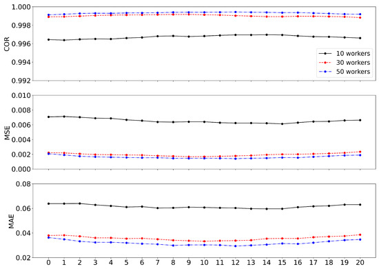
Figure 2. $COR\left(t\right)$, $MSE\left(t\right)$, and $MAE\left(t\right)$ results for the datasets with the cases $N_w=10,30,50$ for each time $t\in {\left[T\right]}_0$.

Figure 3 presents the true and estimated abilities for each group $i\in \left[G\right]$ for the first dataset of the case $N_w=50$. The true abilities tend to lie within the $\pm 2$ standard deviation of the $L=200$ particle sequences, implying that the presented algorithm estimates the true abilities very well. The results for groups 1 and 6 indicate that the estimates can capture increasing or decreasing patterns as well. Figure 3 on the right-hand side shows the analogous plot for the working rate given in (1), suggesting that the ability estimates are useful for estimating the working rates. Note that the estimated working rates are quite accurate for a broad range of working rates. In conclusion, the simulation result demonstrates that the estimation/inference works well for both model parameters and workers’ abilities.

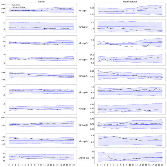
Figure 3. The ability (left) and working rate (right) estimates for all of the groups $i\in \left[G\right]$ of the first dataset in the case of $N_w=50$. The x-axis represents time. The true ability $x_{i,0:T}$ and working rate ${\mu }_{i,0:T}$ for each group $i\in \left[G\right]$ are represented as black solid lines with markers. The estimated ability ${\widehat{x}}_{i,0:T}$ and working rate ${\widehat{\mu }}_{i,0:T}$ values are represented as blue solid lines. The dashed line represents the $\pm 2$ standard deviation of $L=200$ particle sequences for each group.

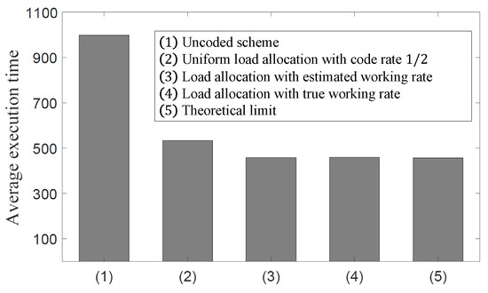
In Figure 4, we compare the expected execution time of the uncoded scheme, the uniform load allocation with code rate $\frac{1}{2}$, the load allocation in (8) with the true working rates, and the load allocation in (8) with estimated working rates. For performance comparisons, the following simulations are conducted with the fixed parameters $m=1$ and $\sigma =1$, ${\sigma }_{ϵ}=0.01$. Moreover, we set $G=2$, $(N_1,N_2)=(20,30)$, $T=20$, and the true working rate $({\mu }_1,{\mu }_2)=(1,5)$ at time $t=0$. At time T, the true working rate varies to $({\mu }_{1,T},{\mu }_{2,T})=(1.0109,4.9999)$. We obtain the estimated working rates of the groups $({\widehat{\mu }}_{1,T},{\widehat{\mu }}_{2,T})=(0.9892,4.8364)$ using the proposed algorithms. This simulation shows that the load allocation in (8) with the estimated working rates can achieve the same performance as the optimal load allocation in (8) with the true working rates. It is also observed that the load allocation in (8) with the estimated working rates shows 54% and 14% reductions in the expected execution times compared to the uncoded scheme and the uniform load allocation with code rate $\frac{1}{2}$, respectively. This result demonstrates that our estimation and the inference of the latent variable are valid in terms of the expected execution time.

Figure 4. Performance comparison between the uncoded scheme, uniform load allocation with code rate $\frac{1}{2}$, load allocation in (8) with the estimated working rates, load allocation in (8) with the true working rates, and the theoretical limit of the expected execution time.

5. Concluding Remarks

In this paper, we model the time-varying ability of workers in heterogeneous distributed computing as latent variables. Since we allow for the ability to change over time, we employ a particle method to infer the latent variables. We present a method for estimating the parameters of the working rate with the latent variable using the EM algorithm combined with sequential Monte Carlo (SMC) for filtering and FFBSa. Monte Carlo simulations verify that the proposed algorithm works reasonably well in estimating the workers’ ability as well as the model parameters. Particularly, the estimation of workers’ ability shows great performance in terms of two measures: COR and MSE between the true and estimated ability.

Exploiting the proposed estimation of the workers’ ability, one can devise the optimal load allocation for minimizing the latency in the heterogeneous distributed computation with workers having time-varying abilities. Numerical simulations show that the load allocation with the estimated working rates achieves the theoretical limit of the expected execution time and reduces the expected execution time by up to 54% compared to existing schemes.

References

- Dean, J.; Corrado, G.; Monga, R.; Chen, K.; Devin, M.; Mao, M.; Senior, A.; Tucker, P.; Yang, K.; Le, Q.V. Large scale distributed deep networks. Proc. Adv. Neural Inform. Process. Syst. (NIPS) 2012, 1, 1223–1231. [Google Scholar]
- Dean, J.; Barroso, L.A. The tail at scale. Commun. ACM 2013, 56, 74–80. [Google Scholar] [CrossRef]
- Lee, K.; Lam, M.; Pedarsani, R.; Papailiopoulos, D.; Ramchandran, K. Speeding up distributed machine learning using codes. IEEE Trans. Inf. Theory 2018, 64, 1514–1529. [Google Scholar] [CrossRef]
- Lee, K.; Suh, C.; Ramchandran, K. High-dimensional coded matrix multiplication. In Proceedings of the 2017 IEEE International Symposium on Information Theory (ISIT), Aachen, Germany, 25–30 June 2017; pp. 2418–2422. [Google Scholar]
- Yu, Q.; Maddah-Ali, M.; Avestimehr, S. Polynomial codes: An optimal design for high-dimensional coded matrix multiplication. In Proceedings of the 31st Conference on Neural Information Processing Systems (NIPS 2017), Los Angeles, CA, USA, 4–9 December 2017; pp. 4403–4413. [Google Scholar]
- Park, H.; Lee, K.; Sohn, J.-Y.; Suh, C.; Moon, J. Hierarchical coding for distributed computing. In Proceedings of the 2018 IEEE International Symposium on Information Theory (ISIT), Vail, CO, USA, 17–22 June 2018; pp. 1630–1634. [Google Scholar]
- Tandon, R.; Lei, Q.; Dimakis, A.G.; Karampatziakis, N. Gradient coding: Avoiding stragglers in distributed learning. In Proceedings of the International Conference Machine Learning, Sydney, Australia, 6–11 August 2017; pp. 3368–3376. [Google Scholar]
- Raviv, N.; Tandon, R.; Dimakis, A.; Tamo, I. Gradient coding from cyclic MDS codes and expander graphs. In Proceedings of the International Conference Machine Learning, Stockholm, Sweden, 10–15 July 2018; pp. 4305–4313. [Google Scholar]
- Ozfaturay, E.; Gündüz, D.; Ulukus, S. Speeding up distributed gradient descent by utilizing non-persistent stragglers. In Proceedings of the 2019 IEEE International Symposium on Information Theory (ISIT), Paris, France, 7–12 July 2019. [Google Scholar]
- Dutta, S.; Cadambe, V.; Grover, P. Coded convolution for parallel and distributed computing within a deadline. In Proceedings of the 2017 IEEE International Symposium on Information Theory (ISIT), Aachen, Germany, 25–30 June 2017; pp. 2403–2407. [Google Scholar]
- Kosaian, J.; Rashmi, K.V.; Venkataraman, S. Learning-Based Coded Computation. IEEE J. Sel. Areas Commun. 2020, 1, 227–236. [Google Scholar] [CrossRef]
- Li, S.; Maddah-Ali, M.A.; Avestimehr, A.S. Coding for distributed fog computing. IEEE Commun. Mag. 2017, 55, 34–40. [Google Scholar] [CrossRef]
- Fu, X.; Wang, Y.; Yang, Y.; Postolache, O. Analysis on cascading reliability of edge-assisted Internet of Things. Reliab. Eng. Syst. Saf. 2022, 223, 108463. [Google Scholar] [CrossRef]
- Zaharia, M.; Konwinski, A.; Joseph, A.D.; Katz, R.H.; Stoica, I. Improving mapreduce performance in heterogeneous environments. In Proceedings of the USENIX Symposium on Operating Systems Design Implement (OSDI), San Diego, CA, USA, 8–10 December 2008; pp. 29–42. [Google Scholar]
- Reisizadeh, A.; Prakash, S.; Pedarsani, R.; Avestimehr, S. Coded computation over heterogeneous clusters. IEEE Trans. Inf. Theory. 2019, 65, 4227–4242. [Google Scholar] [CrossRef]
- Kim, D.; Park, H.; Choi, J.K. Optimal load allocation for coded distributed computation in heterogeneous clusters. IEEE Trans. Commun. 2021, 69, 44–58. [Google Scholar] [CrossRef]
- Gao, J. Machine Learning Applications for Data Center Optimization. Google White Pap. Available online: https://research.google/pubs/pub42542/ (accessed on 6 April 2023).
- Tang, B.; Matteson, D.S. Probabilistic transformer for time series analysis. Adv. Neural Inf. Process. Syst. 2021, 34, 23592–23608. [Google Scholar]
- Lin, Y.; Koprinska, I.; Rana, M. SSDNet: State space decomposition neural network for time series forecasting. In Proceedings of the 2021 IEEE International Conference on Data Mining (ICDM), Auckland, New Zealand, 7–10 December 2021; pp. 370–378. [Google Scholar]
- Hu, Y.; Jia, X.; Tomizuka, M.; Zhan, W. Causal-based time series domain generalization for vehicle intention prediction. In Proceedings of the 2022 International Conference on Robotics and Automation (ICRA), Philadelphia, PA, USA, 23–27 May 2022; pp. 7806–7813. [Google Scholar]
- Jung, H.; Lee, J.G.; Kim, S.H. On the analysis of fitness change: Fitness-popularity dynamic network model with varying fitness. J. Stat. Mech. Theory Exp. 2020, 4, 043407. [Google Scholar] [CrossRef]
- Kitagawa, G. Monte Carlo filter and smoother for non-Gaussian nonlinear state space models. J. Comput. Graph. Stat. 1996, 5, 1–25. [Google Scholar]
- Kantas, N.; Doucet, A.; Singh, S.S.; Maciejowski, J.; Chopin, N. On particle methods for parameter estimation in state-space models. Stat. Sci. 2015, 30, 328–351. [Google Scholar] [CrossRef]
- Pitt, M.K.; Shephard, N. Filtering via simulation: Auxiliary particle filters. J. Am. Stat. Assoc. 1999, 94, 590–599. [Google Scholar] [CrossRef]
- Carpenter, J.; Clifford, P.; Fearnhead, P. Improved particle filter for nonlinear problems. IEE Proc. Radar Sonar Navig. 1999, 146, 2–7. [Google Scholar] [CrossRef]
- Doucet, A.; De Freitas, N.; Gordon, N. An introduction to sequential Monte Carlo methods. Seq. Monte Carlo Methods Pract. 2001, 3–14. [Google Scholar] [CrossRef]
- Doucet, A.; Johansen, A.M. A tutorial on particle filtering and smoothing: Fifteen years later. Handb. Nonlinear Filter 2009, 12, 656–704. [Google Scholar]
- Gilks, W.R.; Wild, P. Adaptive rejection sampling for Gibbs sampling. Appl. Statist. 1992, 41, 337–348. [Google Scholar] [CrossRef]
Disclaimer/Publisher’s Note: The statements, opinions and data contained in all publications are solely those of the individual author(s) and contributor(s) and not of MDPI and/or the editor(s). MDPI and/or the editor(s) disclaim responsibility for any injury to people or property resulting from any ideas, methods, instructions or products referred to in the content. |
© 2023 by the authors. Licensee MDPI, Basel, Switzerland. This article is an open access article distributed under the terms and conditions of the Creative Commons Attribution (CC BY) license (https://creativecommons.org/licenses/by/4.0/).