Featured Application
Radiation thermometry of real objects under real conditions.
Abstract
Despite great technical capabilities, the theory of non-contact temperature measurement is usually not fully applicable to the use of measuring instruments in practice. While black body calibrations and black body radiation thermometry (BBRT) are in practice well established and easy to accomplish, this calibration protocol is never fully applicable to measurements of real objects under real conditions. Currently, the best approximation to real-world radiation thermometry is grey body radiation thermometry (GBRT), which is supported by most measuring instruments to date. Nevertheless, the metrological requirements necessitate traceability; therefore, real body radiation thermometry (RBRT) method is required for temperature measurements of real bodies. This article documents the current state of temperature calculation algorithms for radiation thermometers and the creation of a traceable model for radiation thermometry of real bodies that uses an inverse model of the system of measurement to compensate for the loss of data caused by spectral integration, which occurs when thermal radiation is absorbed on the active surface of the sensor. To solve this problem, a hybrid model is proposed in which the spectral input parameters are converted to scalar inputs of a traditional scalar inverse model for GBRT. The method for calculating effective parameters, which corresponds to a system of measurement, is proposed and verified with the theoretical simulation model of non-contact thermometry. The sum of effective instrumental parameters is presented for different temperatures to show that the rule of GBRT, according to which the sum of instrumental emissivity and instrumental reflectivity is equal to 1, does not apply to RBRT. Using the derived models of radiation thermometry, the uncertainty of radiation thermometry due to the uncertainty of spectral emissivity was analysed by simulated worst-case measurements through temperature ranges of various radiation thermometers. This newly developed model for RBRT with known uncertainty of measurement enables traceable measurements using radiation thermometry under any conditions.
1. Introduction and Literature Review
Since the SARS outbreak in China in 2002, influenza A (H1N1) in 2009, Ebola virus disease (EVD) in 2014 and coronavirus disease in 2019 (COVID-19), when non-contact thermometry was mainly recognized as a practically convenient method for measurement (screening) of human body temperature [1,2,3,4,5], radiation thermometry has continuously expanded to new industries and applications, including the consumer market. Thanks to the progress in the production of thermal radiation sensors in recent decades, the instrumentation in the field of radiation thermometry is now technologically advanced. However, there are also studies available which demonstrate the limitations of the non-contact thermometry [6,7,8,9,10,11].
Despite practical advances, the theory of radiation thermometry with spectral-band sensors has not advanced in recent years. While non-contact temperature measurements are in practice often conducted on simplified grey bodies, no methodology has yet been developed for measuring the temperature of real bodies. The authors of this article strive to introduce traceability into the practice of radiation thermometry of real bodies. To achieve traceable measurements under real conditions, a mathematical model of measurement must be derived and measurement uncertainty evaluated.
1.1. Black Body Radiation Thermometry (BBRT)
A black body (BB) is an ideal radiation source that has a maximum (or ideal, perfect) emissivity value (of 1) at all wavelengths () and in all directions, and does not reflect incident radiation. Therefore, the result of a non-contact temperature measurement on a black body always corresponds only to the temperature of the object and is independent of other environmental influences (neglecting the influence of the atmosphere).
While traceability is easily obtained with such measurements, the black body radiation thermometry (BBRT) method is only applicable to measurements on black bodies, which is an idealization of real properties and only suitable (with negligible effects) when laboratory black bodies are used. In practice, laboratory black bodies are the best approximation of the black body with the highest achievable emissivity, which ideally approaches the emissivity of the theoretical black body (). Despite the ease of measurement, black bodies are difficult to achieve in practice and are usually not feasible.
Established protocols for calibration of non-contact temperature measuring instruments, and consequently most scientific publications in this field, mostly refer to calibrations of radiation thermometers using black bodies. Such calibration protocols are described in [12,13,14,15,16,17,18,19]. BBRT is considered traceable and is therefore used by calibration laboratories to transfer radiation references. This means that black body calibrations are used to transfer reference measurements from the highest levels of traceability to lower levels.
The BBRT model is used by the simplest measuring instruments that operate with a fixed instrumental emissivity value of 1 (e.g., transfer reference thermometers and many industrial sensors), and is also available in the majority of radiation thermometers, which have adjustable instrumental parameters that can be set to a value of 1.
1.2. Grey Body Radiation Thermometry (GBRT)
Grey body radiation thermometry (GBRT) is a simplification used for measuring grey bodies. It assumes that all influential quantities in the system of measurement are spectrally homogeneous and therefore independent of the observed wavelength. Based on this simplification, the spectral behaviour can be summarized with scalar values (constants), and their effect can be considered spectrally independent.
While GBRT is theoretically similar to BBRT in terms of scalar calculation algorithm, it extends the application of radiation thermometry to idealized real bodies—grey bodies.
GBRT requires scalar input parameters, generally referred to as instrumental parameters, which enable compensation of inevitable environmental influences. Input parameters should correspond to the entire system of measurement, which consists of the measured object (and its temperature), the environmental radiation, the transfer path and the measuring instrument. In GBRT, only the influence of actual grey bodies, which are spectrally independent, can be correctly compensated.
The GBRT model and its variations are currently used by most radiation thermometers on the market with an adjustable emissivity parameter. This approach has been documented in numerous non-scientific (e.g., Fluke 4181 calibrator manual [20]) and scientific [21] sources and thoroughly by Saunders [22], who modelled the response of a fixed instrumental emissivity radiation thermometer in calibration with a black body calibrator. Although the article focuses on calibration, the mathematical model is also applicable to measurements. The grey body model by Saunders utilized radiances (total radiant powers throughout the spectrum, denoted ), obtained by the Sakuma–Hattori approximation of Planck’s law. Spectral interactions are not considered later in this model, limiting model performance to spectrally homogenous influence properties of GBRT.
1.3. Real Body Radiation Thermometry (RBRT)
Some authors previously attempted to incorporate the emissivity characterisation within correction of thermal calibration by expressing common parameters [23]; however, such solutions are not applicable upon a change of environmental conditions and require re-calibration.
Currently, best practice in radiation thermometry of real bodies (RBRT) is to adjust the input parameters of the GBRT model while matching the measurement and reference temperature of the surface, obtained with a contact thermometer.
Repeated evaluations of required instrumental parameters are required even in radiation thermometry of grey bodies because of the thermal dependence of spectral influence parameters. While thermal dependence of influence parameters is documented for many materials and often expected in practice, spectral interactions of spectral influence parameters in the system of measurement are always neglected in the GBRT model; therefore, GBRT is not suitable for RBRT, where spectral parameters are non-homogenously distributed.
In order to correctly perform RBRT, instrumental parameters of GBRT should take into account the spectral distribution of influence parameters and the spectral radiances that are emitted and absorbed at each stage of the physical process of RBRT.
The objective of this study was to define a mathematical model for the process of radiation thermometry (including BBRT, GBRT and RBRT) and to define inverse models that serve to compensate for the inevitable influences within the physical model, namely emission, reflection and atmospheric transmission.
2. The Direct (Physical) Model of Radiation Thermometry
2.1. The Full System of Measurement
In radiation thermometry, thermal radiation from objects is transferred to the radiation thermometer according to the physical laws of radiation. In measurement systems, influences of the environment are usually inevitable; therefore, these influences are taken into account and compensated for in the measuring instrument. These influences include reflection, transmission through the air (and possibly optics and filter) and absorption to the sensor surface (Figure 1).
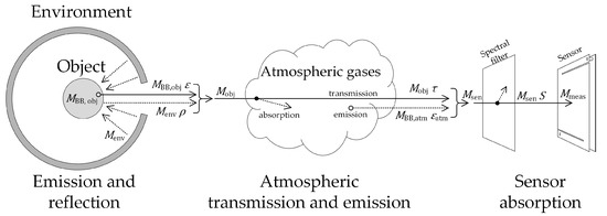
Figure 1.
Physical system of measurement in radiation thermometry with key influence parameters. Physical quantities and their notation correspond to Equation (3).
Radiation thermometer sensors measure the object’s radiant heat flux to its surface. Conventional thermometers use thermal sensors that absorb radiation on an exposed, absorbing surface, and convert it to thermal radiation. This is the case with the most commonly used types of thermopile: MEMS and pyroelectric sensors.
The temperature difference between the exposed and the unexposed side of the absorbing surface is measured and calculated to the incident heat flux, using characteristic functions of the sensor that are beyond the scope of this research and are considered properly calibrated and traceable. The self-emission of the sensor is considered mathematically correctly compensated within the scope of this research, as it is purely dependent on the temperature of the sensor.
The output data of the sensor and the complementary input–output characteristic of the sensor constitute the incident radiance, which is assumed as compensated for natural heat dissipation, both through the case and through the optics. These influences are considered mathematically easy to compensate for, and are beyond the scope of this research.
The incident radiance data of the sensor are later converted by another mathematical model (within the instrument) into the temperature of the radiation source, taking into account the inevitable influences of the environment and reflective properties of the object.
The operation and behaviour of the latter model, which is the inverse of the physical model, is the subject of this article. It represents the opposite of the physical model of radiation transfer, described in Figure 1.
2.2. Thermal Radiation Emission, Transfer and Absorption
Every black body with a thermodynamic temperature emits thermal radiation in the form of spectral radiance (Figure 2) in accordance with Planck’s law (1),
where is the Planck constant, is the Boltzmann constant, is the speed of light in the medium and is the wavelength.
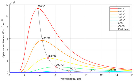
Figure 2.
Spectral radiance emitted by the black body, according to Planck’s law (1).
The actual emission of any real surface is the emission of the black body (2), spectrally reduced by the spectral emissivity of the surface.
A general form for radiation of any real object is described by Equation (3), where represents object’s raw black body emission (2) under an assumption of homogenous temperature; represents incident environmental radiation which is reflected from the surface of a medium; represents spectral radiance behind the object in the case of transmission through a translucent material; and , and represent spectral transmissivity, spectral emissivity and spectral reflectivity of the object, respectively.
Interaction of incident radiation with a medium at any wavelength is described by the equilibrium Equation (4).
According to Kirchhoff’s law [24], emissivity is equal to absorptivity at individual wavelengths (5).
2.3. Input Data of the Physical Model
2.3.1. Object’s Emission and Environmental Radiation Reflection
Equation (6) represents the emission of the surface in the direct model as the spectral radiance of a black body from Equation (2), reduced by the spectral emissivity factor .
According to Equation (4), the only complementary process of emission for real opaque surfaces is reflection. The radiation (7) reflected from the object is considered as being the raw environmental spectral radiance , reduced by the spectral reflectivity factor (8).
The directional dependence of any influence parameter is omitted from this (simplified) model and is considered accounted for in the raw environmental radiation data. This simplification does not affect the performance of the model, as long as the environmental radiation data are obtained in agreement with the spatial reflectivity characteristic of the surface in the given direction of observation.
The directional spectral emissivity of any material can be measured with IR spectroscopy. Databases exist that cover the directional spectral emissivities of various materials, such as ECOSTRESS [25] (formerly ASTER [26]) and USGS Spectral Library Version 7 [27]. The normal (perpendicular) spectral emissivity of Topaz from the USGS Spectral Library is used as an example in this research (Figure 3).
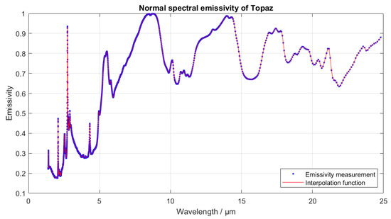
Figure 3.
Example of normal spectral emissivity of Topaz (sample from site 3) from USGS Spectral Library [27].
2.3.2. Atmospheric Transmission and Self-Emission
The emitted and reflected radiation of the object travels through the atmosphere toward the radiation thermometer. During travel, the radiation is partially absorbed according to the spectral absorptivity of the air, while most of the radiation is transmitted according to the spectral transmissivity of the air . According to Kirchhoff’s law (5), spectral absorptivity equals spectral emissivity, therefore atmospheric self-emission is present and can be considered as black body emission (10) reduced by the spectral emissivity of the atmosphere (11).
The spectral transmissivity of the atmosphere is relatively high under usual indoor conditions, as already determined by the authors for the purpose of this study [28]. The spectral transmissivity of air is shown in Figure 4 for a 10 m atmospheric path; however, a 1 m measuring distance—along with 45% relative humidity, 1013.25 hPa atmospheric pressure and 25 °C atmospheric temperature—is used for calculations in this article.
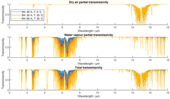
Figure 4.
Spectral transmissivity of dry air, water vapour and combination of both from author’s previous publication [28]. Displayed spectra correspond to 1013.25 hPa atmospheric pressure and 10 m atmospheric path, calculated at 0.01 μm resolution.
2.3.3. Optical System of the Measuring Instrument
The transmission path may also include possible transparent windows and the optical system of the thermometer. Publicly available spectral data of the optics of pyrometers and thermal imagers are limited; however, the properties of the optics are usually included in the spectral sensitivity characteristic of the measuring instrument.
Remaining radiances, detected by the sensor and originating within the measuring instrument, including the optical system, are considered device-compensated and outside the scope of this research.
2.3.4. Sensor Absorption and Characteristic Function
The combined spectral radiance travelling towards the measuring instrument is absorbed at the sensor. The actual detected (measured) spectral radiance to the sensor shown in Figure 1 prior to integration is the incident spectral radiance to the sensor , reduced by the sensor’s relative spectral sensitivity . Relative spectral sensitivity is used exclusively in this research. Absolute scaling is considered as accounted for in sensor calibration and does not influence the operation of the models.
Figure 5 presents the relative spectral sensitivity of the Heitronics KT19.01 and two temperature ranges of the Heitronics Transfer Radiation Thermometer II (TRT II), digitized from Heitronics pyrometer documentation [29], and the generic spectral sensitivity of vanadium oxide (VOx)-based microbolometer detectors of FLIR thermal imagers with 45° field-of-view optics [30].
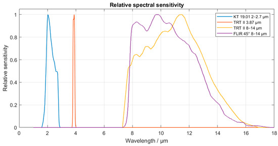
Figure 5.
Spectral sensitivity of Heitronics KT19.01 and the high and the low temperature range of Heitronics Transfer Radiation Thermometer II (TRT II), digitized from Heitronics pyrometer documentation [29], and generic spectral sensitivity of vanadium oxide (VOx)-based microbolometer detectors of FLIR thermal imagers with 45° field-of-view optics [30].
Analytical solutions for the integration of Planck’s law are complex, impractical, and moreover infeasible when the discretely measured spectral sensitivity of the sensor and other influence parameters are taken into account. For this reason, we have opted for entirely numerical calculations.
A sensor’s characteristic function converts from the input quantity to the output quantity. The characteristic function is usually obtained by calibration. Sensors for thermal radiation convert the radiance to an electrical response, generally obtained numerically as a sensor reading.
However, in radiation thermometry, radiance is measured by integration of spectral radiance, according to Equation (13). Calibrations are usually limited to black bodies and therefore the input quantity of a sensor characteristic function is usually extended from radiant power to the temperature of a black body radiator. This assumption utilizes Planck’s law (1) for the missing relationship between the spectral radiance and the temperature of a black body.
For the purpose of this research, the output quantity of the sensor is considered correctly calibrated as the radiance of a black body , detected at the sensor in W sr−1 m−2. The sensor characteristic function is presented in Figure 6.
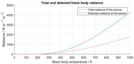
Figure 6.
The total radiance of a black body source at different temperatures and the actual detected radiance at the sensor, forming the sensor characteristic function. VOx sensor sensitivity from Figure 5 was used for this plot.
2.4. Constructed Direct Model of Radiation Thermometry
In radiation thermometry, numerous parameters interfere with the signal of interest, namely the radiation emitted by the surface of the measured object. Considering the described properties of the physical laws, a direct model of radiation thermometry can be generated according to Figure 1. Equation (14) represents the direct model of radiation thermometry.
The process flow of the direct model of radiation thermometry is also presented in Figure 7. The spectral information is lost during the spectral integration during absorption on the active surface of the sensor.
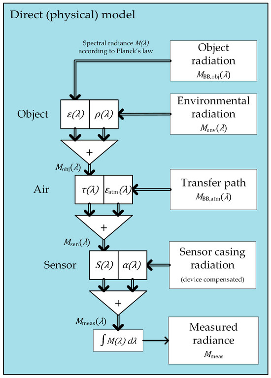
Figure 7.
The direct (physical) model of radiation thermometry, describing the physical process of thermal emission, propagation, absorption and measurement of object (spectral) radiance. The rectangles represent the black body emissions, while the square and triangular operators represent the scaling and summation for the (spectral) radiance. The arrows with the double lines represent the spectral radiance, while the single-line arrows represent the radiance (the total radiant power without spectral information).
Individual contributions can be expressed (15).
2.5. Final Spectral Data of the Physical Model
A theoretical example of spectral behaviour within the direct model (14) is presented in Figure 8. A spectral emissivity characteristic was randomly generated for this research, which is intentionally non-homogeneous across the entire sensitivity spectrum of the sensor to emphasize the effect of non-homogeneous spectral emissivity, as can occur with real objects.
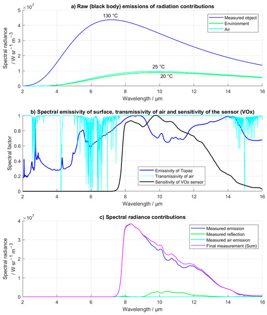
Figure 8.
Shown is the spectrally simulated behaviour of the direct model with (a) the raw spectral radiance of black body emissions; (b) the spectral emissivity of surface, the spectral transmissivity of the air, and the spectral sensitivity of the sensor; and (c) the partial and total spectral radiance, as absorbed in the sensor. The area under the sum of all contributions represents the signal output from the sensor.
Figure 8a presents the raw spectral radiances , and of the three contributing sources of radiation. Figure 8b presents the influence parameters , and . Figure 8c presents the detected spectral radiance of the three contributing sources, as expressed in Equation (15) prior to integration, and the sum of the three, as expressed in Equation (14) prior to integration.
3. The Inverse Model of Radiation Thermometry
3.1. Derivation of the Inverse Model of Radiation Thermometry
The direct model is based on a real physical model of conversion of object temperature to radiant power as a sensor value, including the inevitable influences of the environment. The inverse model, i.e., the inverse of the physical model, is used for the calculation from the radiant power on the sensor to the temperature of the object.
In all inverse models, inevitable influences of the measured object, environment and air, must be calculated and compensated for from the measured radiance. After compensating for these influences, only the black body radiation of the measured object should be present in the resulting signal as raw surface emission , used in Equation (6) in the direct model (of the real system of measurement). This pure black body emission from Equation (1) can be converted to the object temperature using a black body radiance characteristic function, which is theoretically the inverse of the spectrally integrated Planck’s law.
3.1.1. Theoretically Ideal Spectral Direct and Inverse Models
Since the physical model is a spectral model, the inversion of this model results in a spectral inverse model. The correct combination of the direct and inverse models is shown in Figure 9. Spectral radiance is extinct at the sensor; therefore, the ideal traceable measurements should be made in spectral radiance, not radiance. The ideal direct and inverse models should omit spectral integration; therefore, such a model is not practically feasible with radiance sensors.
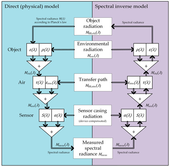
Figure 9.
Theoretically ideal inverse of the direct model. Note that spectral integration is irreversible upon measurement. Therefore, measurement of spectral radiance is required for the ideal inverse model. Spectral integration was omitted from the direct model.
3.1.2. Scalar Inverse Model
Due to spectral data loss at the sensor, most existing radiation thermometers and thermal imagers currently operate with radiances instead of spectral radiances and use the simplified scalar inverse model (Figure 10) and its derivatives. A scalar model is a generalization, used because the sensor reading is obtained as radiance (radiant power), which is a scalar number, rather than spectral radiance, which is defined as a spectrally distributed radiant power.
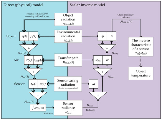
Figure 10.
Model of radiation thermometry with the scalar inverse model. Parameters, beginning with i correspond to scalar instrumental parameters. Dotted lines represent transfer of non-radiation scalar data, such as temperature or calculated scalar equivalent of an influence parameter. The inverse black body radiance characteristic is a characteristic transformation between emitted radiance and temperature of a black body, which can be derived from Planck’s law.
The scalar inverse model can be obtained from the scalar direct model (16); that is, the direct model (14) with scalar influence parameters (, , etc.). This scalar replacement can only be correctly implemented in the direct model under simplification of constant (spectrally independent) influence parameters. The spectrally homogenous (grey) properties of the model, which are required for correct operation, limit the applicability of this model to GBRT.
Assuming an opaque surface, the raw emission of the object can be considered as the emission of a black body of temperature (2). Simplifying for single (homogenous) atmospheric temperature , the raw radiant contribution of the atmosphere can similarly be considered as the emission of a black body (10).
Raw environmental reflection can be simplified as the single temperature emission of a black body as well; however, under real conditions, the incident environmental spectral radiance is a sum of many incident radiances around the measured surface, determined according to the directional reflectivity characteristic of the observed object.
The black body sensor temperature to radiance characteristic of a sensor , obtained in Equation (13), can be expressed from the scalar direct model. Similarly, sensor sensitivity-weighted environmental radiance can be expressed.
By expressing , the scalar inverse model of GBRT can be obtained (18). Parameters marked with the prefix - (e.g., ) are scalar input parameters of the inverse model, called instrumental parameters. These parameters—instrumental emissivity, instrumental reflectivity, instrumental (atmospheric) transmissivity and instrumental atmospheric emissivity—represent the scalar input settings of an instrument’s mathematical model.
The process flow chart of the scalar inverse model is presented in Figure 10.
The temperature measurement can be obtained by inverting the sensor characteristic function , which is obtained from Equation (13) and displayed in Figure 6. The inverse sensor characteristic function is presented in Figure 11.
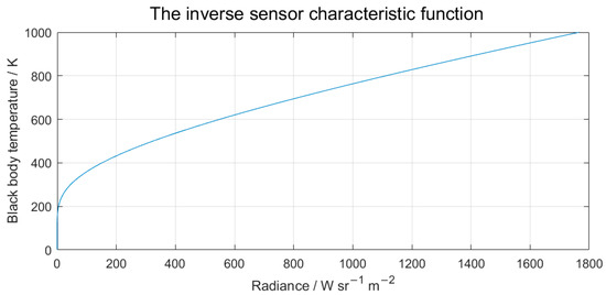
Figure 11.
The inverse characteristic function of a VOx sensor. The characteristic is obtained by inverting the characteristic function of the sensor from Equation (13) and Figure 6.
As a scalar simplification, this model is appropriate for grey GBRT and inherently for BBRT, where interactions are not spectrally dependent. The vast majority of instruments in the field of radiation thermometry currently operate according to this model, as can be seen from the scalar input values.
Since the settings of the measuring instruments are often unknown, these input parameters are usually estimated, taken from literature or determined experimentally, usually without following the rules of traceability for the particular system of measurement. It is also common procedure to use constant instrumental parameters for all measurements of a given surface, regardless of the temperatures and spectral interactions involved.
Due to the omission of processing of the spectral information of the signal, this model and method are considered inaccurate. An improved version of this model is needed to take full advantage of the available accuracy and traceability of radiation thermometry. To do this, the spectral interactions must be accounted for in the inverse model.
3.1.3. Hybrid Model
While an ideal inverse for measurements under real conditions is not possible due to the loss of spectral data in sensor measurement, correct integration of the scalar inverse model for radiation thermometry of real bodies in real conditions (RBRT) can be achieved by correctly accounting for the influence of spectral parameters in instrumental parameters, according to Figure 12.
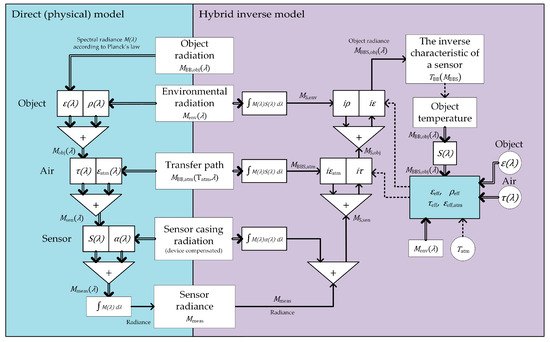
Figure 12.
Hybrid inverse model utilizes effective parameter calculation according to spectral radiances in the system of measurement.
Since the spectral distribution data of the signal are lost in the direct model, it should be accounted for by the effective scalar factor to compensate for the discrepancy between the results of the scalar and the spectral inverse model (19).
These effective scalar parameters correspond to the actual effect of spectral influence parameters on spectral radiances in the direct model (14), as manifested in the measuring instrument.
Since the effective emissivity depends on the spectral radiance of the raw (black body) emission and thus on the temperature of the object, which at the time of measurement is unknown, a recursive relationship is established between the spectral representation of the object’s emission and its temperature. The calculated object temperature can thus be improved iteratively. It is important to note that optimization is only required to better define the spectral distribution of the signal. Therefore, small deviations and fast regression to the optimal results are expected from the model throughout iterations; however, at least two iterations are required to vaguely approximate the spectral distribution of the object’s (temperature-dependent) raw emission.
By definition, spectral influence parameters are defined as the ratio between the real and hypothetically ideal radiant response (i.e., emission, reflection, transmission, absorption) at individual wavelengths. A scalar influence parameter corresponds to the ratio of the actual and theoretically ideal radiance. In terms of radiation thermometry, these radiant contributions correspond to the measured (spectral) radiance, as detected by the sensor with spectral sensitivity .
A theoretically accurate implementation of spectral influence parameters in the scalar inverse model can be achieved by expressing with an effective (scalar) factor the overall effect of the spectral influence parameter on the measurement, as detected by the sensor. For this, the direct model of radiation thermometry (14) can be utilized. By taking into account Planck’s law for an object’s raw (black body) emission, spectral influence parameters and possibly other spectral radiances in the system of measurement (e.g., environmental reflection, atmospheric emission), spectral radiance contributions can be expressed for any stage of the direct (physical) model (14).
First, the effective transmissivity and emissivity of the atmosphere can be expressed. The effective transmissivity corresponds to the radiance of the joint emission and reflection of the atmosphere, whereas the effective emissivity of atmosphere corresponds to the spectral radiance of atmospheric emission.
The effective parameter (e.g., ) is obtained through substitution of a spectral parameter with an effective parameter in the direct model (14) while retaining the result. This is achieved by equating a direct model with the spectral parameter and a direct model with the spectral parameter substituted for an effective scalar (e.g., in Equation (21)). Independent contributions (e.g., emission of atmosphere) are equal on both sides of equation and can therefore be subtracted from expression.
Expressing from Equation (21), effective transmissivity can be expressed.
For advanced use, effective transmissivity can be separated into two entities (23) and (24), according to the direct model, each with individual contributions (15) corresponding to its own contributing emitter and spectral distribution of the affected radiance.
Similarly, the effective atmospheric emissivity (25) can be calculated.
Continuing substitutions in Equation (20), the effective emissivity (26) and reflectivity (27) can be expressed. As effective transmissivity corresponds to influenced radiances, including emissivity and reflectivity, it can substitute for spectral transmissivity and can be, as a constant, expressed outside the integral and reduced from both sides of the division.
A rule can be derived for converting any spectral influence parameter to effective scalar value (28), which allows the calculation of any effective factor under any conditions and in any phase of the direct model. The effective scalar value is equal to the ratio between the actual measured radiance and the ideal radiance of the direct model (14), as it would be measured if the influence parameter was ideal, i.e., a value of 1.
Spectral weights or (29) for averaging of spectral parameters can be expressed from Equations (22) and (25)–(27) and generated for different detectors and black body emissions, as shown in Figure 13. Spectral weights display spectral representation of the given parameter in the final measurement.
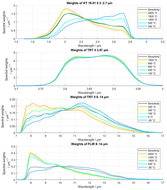
Figure 13.
Spectral weights for averaging of the spectral emissivity for different sensors. Spectral weights were calculated according to Equation (29) using spectral sensitivities from Figure 5 and black body emission according to Equation (1). Note that with the spectral shift of the peak of the spectral radiance to the wavelengths outside the sensitivity range of the sensor, the instrumental emissivity spectral representation is less sensitive to temperature variations.
Detectors with different spectral sensitivities differently respond to anomalies in spectral parameters due to temperature-induced shifts in radiance.
4. Results
4.1. Validation of the Hybrid Inverse Model of Radiation Thermometry
A measurement by radiation thermometry was simulated with a scalar and a hybrid inverse model. The model errors shown in Figure 14 are defined as measurement errors, calculated as the difference between the simulated theoretical measured temperature and the reference temperature of the object used for the simulation.
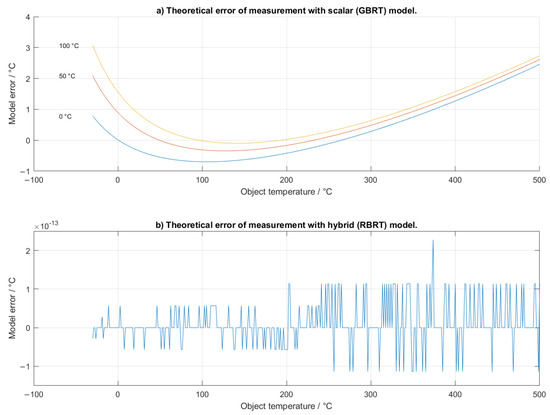
Figure 14.
Theoretical error of grey body (GBRT) and real body (RBRT) radiation thermometry models, using inverse model (a) with constant parameters, spectrally averaged from 8 to 14 μm at various environmental temperatures; and (b) effective parameters, weighted to the signal and the instrument in accordance with the hybrid inverse model. The model error of the hybrid model does not change with environmental temperature and can be easily further decreased by improving the resolution of the inverse characteristic function, obtained as function fit in Figure 11.
The model with constant instrumental values, obtained by the averaging of the spectral parameters, had large model errors. The model with effective scalar values, calculated for the signal and the instrument according to Equation (28), had negligible error.
4.2. Effective Parameters as Instrumental Settings for the Scalar Inverse Model
The equilibrium equation () is in practice usually extended to scalar operators (). This simplification is correct only if the measured surface is an ideal (spectrally homogenous) grey body or if the spectral distributions of the signals involved are equal, i.e., in thermal equilibrium.
Under real conditions, the effective scalar equivalent value of a spectral parameter is determined by the spectral distribution of the spectral parameters, the signal, and the spectral sensitivity of the instrument. Since the spectral parameters are represented according to the signals involved, the effective scalar parameters are independent and therefore the sum of the three instrumental parameters is not necessarily equal to 1 when measured under real conditions. The effective and mean scalars of the emissivity and reflectivity of the object are shown in Figure 15, where each of the parameters is expressed as a function of the influenced value, in this case the temperature of the emitting object and the temperature of the environment, assuming thermal equilibrium of the environment, which is necessary to satisfy the assumption that the radiance is distributed according to Planck’s law.
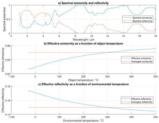
Figure 15.
Shown are (a) the spectral emissivity and spectral reflectivity of the measured surface; (b) the spectrally averaged (8–14 µm) and effective emissivity as a function of the temperature of the measured object; and (c) the spectrally averaged (8–14 µm) reflectivity and effective reflectivity as a function of the environmental temperature, assuming pure emission according to Planck’s law, e.g., when the environment has (a single) homogeneous temperature. Thermally non-homogenous environments are expected under real conditions, in which case, spectral radiance of the environment can be either measured or theoretically derived by summation of emission for this calculation method.
Unlike in the theory of radiation thermometry for grey bodies, the sum of effective parameters in the radiation thermometry of real objects is not necessarily equal to 1. This is evident in Figure 16, where the sum of the two effective parameters is plotted as a function of the object and environmental temperature.
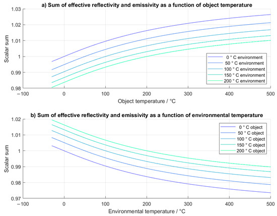
Figure 16.
Sum of effective scalar emissivity and reflectivity with (a) object and (b) environmental temperature. Multiple plots show variation of (a) environmental and (b) object temperature.
The transmissivity was set to 0 and omitted for opaque bodies. Considering that the model error, obtained from the plotted effective parameters in Figure 14b was negligible, the effective parameters are considered valid.
The sum of the effective atmospheric emissivity and the transmissivity at fixed atmospheric temperature (Figure 17) also deviates from 1, but the effect is less pronounced.
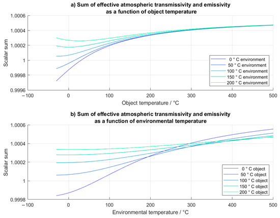
Figure 17.
The sum of effective atmospheric transmissivity and emissivity with (a) object temperature and (b) environmental temperature, assuming a thermally homogeneous environment. Multiple plots show the variation of (a) environmental temperature and (b) object temperature.
4.3. Measurement Uncertainty Due to Uncertainty of Emissivity
The use of grey body measurement principles under real conditions is currently the standard practice in the field of radiation thermometry. Since the grey body simplification of spectral homogeneity never applies under real conditions, the uncertainty of spectral emissivity must be accounted for in the uncertainty of non-contact temperature measurement.
The highest measurement deviations are expected when the spectral parameter (emissivity) is at its highest deviation along the full (measurement) spectrum. Deviations of spectral emissivity in narrow spectral bands always produce a lesser or equal effect than deviations along the full spectrum (of measurement). Therefore, spectrally local uncertainties of the spectral emissivity are considered to be included in the uncertainty budget of the uncertainty interval of the total spectrum. Therefore, the calculation of the measurement of uncertainty interval is performed as the worst-case study, where the highest and the lowest expected deviation of the spectral emissivity (over the whole spectrum) define the uncertainty interval at the output of the measurement process.
Figure 18 shows the uncertainty intervals of GBRT due to the uncertainty of emissivity. Although a (spectrally homogeneous) grey body was used in this figure, any case-specific (spectral) emissivity and the corresponding (spectral) uncertainty can be used for the uncertainty calculation. In such a case, the highest possible uncertainty should be used.
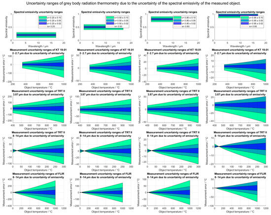
Figure 18.
Measurement uncertainty intervals for grey body radiation thermometry of surfaces with different spectral emissivities and homogeneities. The uncertainty contributions are calculated at 25 °C environmental temperature and correspond to the probability of occurrence of the spectral emissivity within the specified uncertainty interval.
Similarly, the ranges of relative uncertainty are shown in Figure 19. The relative uncertainty is expressed as the ratio between the total measurement uncertainty and the temperature difference between the object and the reflected environment.
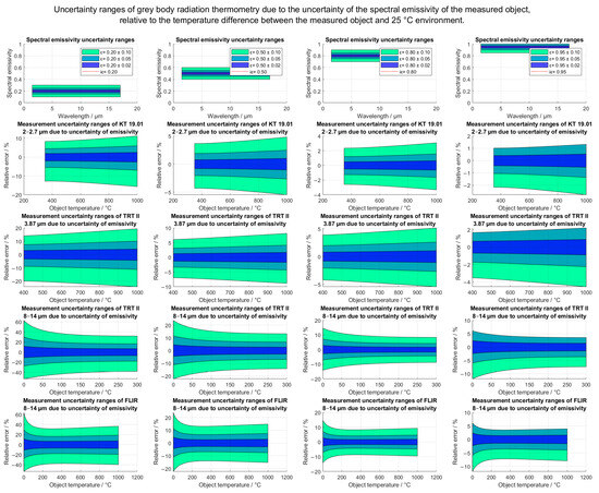
Figure 19.
Relative measurement uncertainty intervals for grey body radiation thermometry of surfaces with different spectral emissivities and homogeneities, expressed relative to the temperature difference between the measured object and the 25 °C environment. The uncertainty contributions correspond to the probability of occurrence of the spectral emissivity within the specified uncertainty interval. The singularity of the relative error at temperature 25 °C due to the division of the absolute error with 0 °C thermal difference was omitted. If the temperature of the object and the reflected radiance are equal, emissivity is irrelevant and the measurement uncertainty due to the uncertainty of the emissivity does not exist.
5. Discussion
5.1. State of the Art in the Field of Radiation Thermometry
Currently the field of radiation thermometry appears to be technologically well supported. Radiation thermometers with state-of-the-art measuring capabilities are available for scientific, professional and consumer use.
Metrological conformity is in practice established for radiation thermometry of black bodies. Calibrations conducted on black body sources are well established and documented in the literature, often also accredited and traceable to national or international standards. Traceable use of radiation thermometers usually only includes BBRT; however, it is often also applied to GBRT while neglecting spectral interactions.
Through theory and scalar inverse models, the use of radiation thermometers can be extended to grey bodies while retaining traceability; however, this is generally not applicable to real conditions. The literature search for theoretically traceable radiation thermometry protocols for real bodies (RBRT) did not yield any existing results.
5.2. The Use of the Equilibrium Equation for Instrumental Settings in Radiation Thermometry under Real Conditions Is Theoretically Incorrect
As demonstrated by the simulation in Figure 15, the effective scalar equivalents of the spectral parameters do not necessarily sum to 1 (Figure 16) under real conditions. Therefore, the usual simplification of the equilibrium equation of the scalar inverse model () is not valid under real conditions, when only a slight spectral non-homogeneity of the spectral factors exists.
The use of this equation under real conditions inevitably results in errors since the data of the spectral distribution of the signals are not taken into account, as shown in Figure 14.
5.3. Theoretically Derived Direct (Physical) Model and Hybrid Inverse, Validated by Simulation
Based on the results of literature review, a physical model of radiation thermometry was defined and scalar and hybrid inverse models were derived.
To correctly account for the interactions between the spectral distributions of the influence parameters and the involved signals, the hybrid inverse model should be used where the scalar influence parameters are determined as effective scalar parameters according to Equation (28).
Considering the results of the model error simulation in Figure 14, the hybrid inverse model, where the instrumental parameters are set to the effective values, was validated as a correct approach for radiation thermometry of real objects, resulting in negligible conversion error. This approach requires an individual calculation of the effective scalar equivalent for each spectral parameter and an iterative calculation of the object temperature.
5.4. Uncertainty of Radiation Thermometry Due to Uncertainty of Spectral Emissivity
Each surface can be classified as an idealized grey body with corresponding spectral homogeneity uncertainty. To assure traceability of measurements, input uncertainties must be evaluated and included in the total measurement uncertainty. A demonstration of the evaluation of uncertainty due to spectral emissivity is shown in Figure 18.
In general, the measurement uncertainty of any radiation thermometer is lowest near the apparent temperature of reflection and increases approximately linearly with the difference from the environment temperature. The linearity was explored in Figure 19, where the measurement uncertainty is expressed in relation to the temperature difference between the measured object and the 25 °C environment.
The results in Figure 18 indicate that different sensors with different spectral sensitivities respond differently to measurement uncertainty, presumably due to different emission/reflection ratios in different spectral sensitivity ranges and at different object temperatures.
As can be seen from the simulation results, the measurement uncertainty increases with decreasing emissivity of the surface (at constant input uncertainty of the emissivity).
As the emissivity uncertainty interval approaches an emissivity value of 0, the total measurement uncertainty will seemingly increase to infinity. This is also logical, since non-emissive surfaces cannot be measured due to the lack of emission.
Another error was found to occur frequently when the compensation algorithms overestimate the influence of influence parameters. In this case, the compensated signal may be calculated to a negative incident radiance of the environment. Overcompensation is very problematic when low temperatures (below 0 °C) are measured at higher environmental temperatures. Due to the steepness of the inverse sensor characteristic (Figure 11) at low temperatures, a small uncertainty in the inverse model translates to a high temperature measurement uncertainty. This is evident in Figure 19 for TRT II and FLIR detectors in 8–14 µm range.
Author Contributions
Conceptualization, V.M. and I.P.; methodology, V.M. and I.P.; software, V.M.; validation, V.M.; formal analysis, V.M. and I.P.; investigation, V.M.; resources, V.M. and I.P.; data curation, V.M.; writing—original draft preparation, V.M.; writing—review and editing, I.P.; visualization, V.M.; supervision, I.P.; project administration, I.P.; funding acquisition, I.P. All authors have read and agreed to the published version of the manuscript.
Funding
The authors acknowledge the financial support from the Slovenian Research Agency (research core funding No. P2-0225). The research was also supported partially by the Ministry of Economic Development and Technology, Metrology Institute of the Republic of Slovenia, in scope of contract 6401-18/2008/70 for the national standard laboratory for the field of thermodynamic temperature and humidity.
Institutional Review Board Statement
Not applicable.
Informed Consent Statement
Not applicable.
Data Availability Statement
All data, presented in this study, are publicly available from cited sources. Plot scripts in MATLAB environment are available upon request.
Conflicts of Interest
The authors declare no conflict of interest.
Correction Statement
This article has been republished with a minor correction to the readability of Figure 14. This change does not affect the scientific content of the article.
Nomenclature
| Terminology | |
| Radiation thermometry | a non-contact method of temperature measurement. Specific to this group of measurement methods is indirect temperature measurement using thermal radiation. A mathematical model of indirect measurement is required to correctly calculate the actual temperature of the measured surface |
| Direct model | a subsection of the radiation thermometry model that occurs in the real world as emission, propagation and absorption of spectral radiance |
| Inverse model | a subsection of the radiation thermometry model that occurs in the measuring instrument as compensation of the (inevitable) environmental influences of the direct model |
| Black body radiation thermometry (BBRT) | a method for radiation thermometry where the measurement algorithm assumes black body properties of the measured surface |
| Grey body radiation thermometry (GBRT) | a method for radiation thermometry where the measurement algorithm assumes real (spectrally non-homogenous) properties of the measured surface and other influences |
| Real body radiation thermometry (RBRT) | a method for radiation thermometry where the measurement algorithm assumes real (spectrally non-homogenous) properties of the measured surface and other influences |
| System of measurement | the physical system of the radiation thermometer and all other objects and environmental conditions which influence the measurement of radiance in radiation thermometry |
| Object | refers to the object, or specifically the surface of interest, in radiation thermometry |
| Radiance | the radiant flux emitted, reflected, transmitted or received by a surface, per unit solid angle per unit projected area. Radiance is a directional quantity |
| Spectral radiance | the spectrally defined radiance per unit wavelength |
| Raw spectral radiance | the spectral radiance of a black body, considered to be correctly defined by Planck’s law (1) |
| Raw environmental spectral radiance | the incident spectral radiance of the hemispherical surroundings of the surface, summed according to the directional reflectivity characteristic of the surface |
| Spectral parameters (also factors) | in the scope of this article they are considered as spectrally defined influence parameters, namely emissivity, transmissivity, reflectivity, absorptivity or instrument sensitivity |
| Scalar parameters (also factors) | in the scope of this article they are considered as being parameters, represented with a (single) scalar value. Spectrally homogenous spectral parameters are considered equivalent to scalar parameters |
| Instrumental parameters: | the input parameters of the instrument; in scope of this article, instrumental parameters are considered as being scalar values used in the scalar section of any inverse model of radiation thermometry. |
| Effective parameters | scalar parameters which correspond to (and can substitute for) the spectral parameter in the given system of measurement. A scalar equivalent of a spectral parameter is obtained as a ratio between actual radiant contribution and ideal radiant contribution if the spectral parameter was ideal and set to a value of 1. The scalar equivalent corresponds to the influence of spectral parameter on the ra-diance contribution, as manifested to the radiation thermometer in the given system of measure-ment. In an ideal case, effective parameters are expected to correctly solve the scalar inverse model. |
| Abbreviations | |
| Thermodynamic temperature in Kelvins | |
| Wavelength of electromagnetic radiation in metres | |
| Black body spectral radiance characteristic (Planck’s law) | |
| Raw spectral radiance of measured object, considered as black body emission | |
| Raw environmental spectral radiance before reflection, calculated or measured according to the object’s directional reflectivity characteristic | |
| Raw spectral radiance of the atmosphere in the transfer path, considered as being black body emission | |
| Spectral emissivity of measured surface | |
| Spectral reflectivity of measured surface | |
| Spectral transmissivity of atmospheric path | |
| Spectral emissivity of atmospheric path | |
| Spectrally homogenous (scalar) parameters | |
| Instrumental parameters (scalars) as input parameters of scalar inverse models | |
| Effective parameter values | |
| Spectral sensitivity of the sensor in absolute or relative scale | |
| Measured radiance, as detected by the sensor | |
| Black body radiance characteristic (integral of Planck’s law) | |
| Black body—sensor radiance characteristic | |
| Any parameter (and similarly, spectral or effective variation) | |
| Spectral weights for conversion of spectral to effective parameter | |
References
- Adams, S.D.; Valentine, A.; Bucknall, T.K.; Kouzani, A.Z. Technologies for Fever Screening in the Time of COVID-19: A Review. IEEE Sens. J. 2022, 22, 16720–16729. [Google Scholar] [CrossRef]
- Yang, X.; Yu, Y.; Xu, J.; Shu, H.; Xia, J.; Liu, H.; Wu, Y.; Zhang, L.; Yu, Z.; Fang, M.; et al. Clinical course and outcomes of critically ill patients with SARS-CoV-2 pneumonia in Wuhan, China: A single-centered, retrospective, observational study. Lancet Respir. Med. 2020, 8, 475–481. [Google Scholar] [CrossRef]
- Nishiura, H.; Kamiya, K. Fever screening during the influenza (H1N1-2009) pandemic at Narita International Airport, Japan. BMC Infect. Dis. 2011, 11, 111. [Google Scholar] [CrossRef] [PubMed]
- Chiu, W.; Lin, P.W.; Chiou, H.Y.; Lee, W.S.; Lee, C.N.; Yang, Y.Y.; Lee, H.M.; Hsieh, M.S.; Hu, C.J.; Ho, Y.S.; et al. Infrared Thermography to Mass-Screen Suspected Sars Patients with Fever. Asia Pac. J. Public Health 2005, 17, 26–28. [Google Scholar] [CrossRef] [PubMed]
- Chan, L.-S.; Cheung, G.T.Y.; Lauder, I.J.; Kumana, C.R. Screening for Fever by Remote-sensing Infrared Thermographic Camera. J. Travel Med. 2004, 11, 273–279. [Google Scholar] [CrossRef]
- Yoon, H.W.; Khromchenko, V.; Eppeldauer, G.P. Improvements in the design of thermal-infrared radiation thermometers and sensors. Opt. Express 2019, 27, 14246–14259. [Google Scholar] [CrossRef] [PubMed]
- Liu, C.-C.; Chang, R.-E.; Chang, W.-C. Limitations of Forehead Infrared Body Temperature Detection for Fever Screening for Severe Acute Respiratory Syndrome. Infect. Control Hosp. Epidemiol. 2004, 25, 1109–1111. [Google Scholar] [CrossRef] [PubMed]
- Vardasca, R.; Marques, A.R.; Diz, J.; Seixas, A.; Mendes, J.; Ring, E.F.J. The influence of angles and distance on assessing inner-canthi of the eye skin temperature. Thermol. Int. 2017, 27, 130–135. [Google Scholar]
- Zhou, Y.; Ghassemi, P.; Chen, M.; McBride, D.; Casamento, J.P.; Pfefer, T.J.; Wang, Q. Clinical evaluation of fever-screening thermography: Impact of consensus guidelines and facial measurement location. J. Biomed. Opt. 2020, 25, 097002. [Google Scholar] [CrossRef]
- Machin, G.; Brettle, D.; Fleming, S.; Nutbrownd, R.; Simpsona, R.; Stevensc, R.; Tooleye, M. Is current body temperature measurement practice fit-for-purpose? J. Med. Eng. Technol. 2021, 45, 136–144. [Google Scholar] [CrossRef]
- Goggins, K.A.; Tetzlaff, E.J.; Young, W.W.; Godwin, A.A. SARS-CoV-2 (COVID-19) workplace temperature screening: Seasonal concerns for thermal detection in northern regions. Appl. Ergon. 2022, 98, 103576. [Google Scholar] [CrossRef]
- Murthy, A.V.; Tsai, B.K.; Saunders, R.D. Radiative Calibration of Heat-Flux Sensors at NIST: Facilities and Techniques. J. Res. Natl. Inst. Stand. Technol. 2000, 105, 293–305. [Google Scholar] [CrossRef] [PubMed]
- König, S.; Gutschwager, B.; Taubert, R.D.; Hollandt, J. Metrological characterization and calibration of thermographic cameras for quantitative temperature measurement. J. Sens. Sens. Syst. 2020, 9, 425–442. [Google Scholar] [CrossRef]
- Donlon, C.J.; Wimmer, W.; Robinson, I.; Fisher, G.; Ferlet, M.; Nightingale, T.; Bras, B. A Second-Generation Blackbody System for the Calibration and Verification of Seagoing Infrared Radiometers. J. Atmos. Ocean. Technol. 2014, 31, 1104–1127. [Google Scholar] [CrossRef]
- Boles, S.; Pušnik, I.; Lochlainn, D.M.; Fleming, D.; Naydenova, I.; Martin, S. Development and characterisation of a bath-based vertical blackbody cavity calibration source for the range −30 °C to 150 °C. Measurement 2017, 106, 121–127. [Google Scholar] [CrossRef]
- Kim, H.-I.; Chae, B.-G.; Choi, P.-G.; Jo, M.-S.; Lee, K.-M.; Oh, H.-U. Thermal Design of Blackbody for On-Board Calibration of Spaceborne Infrared Imaging Sensor. Aerospace 2022, 9, 268. [Google Scholar] [CrossRef]
- Miklavec, A.; Pušnik, I.; Batagelj, V.; Drnovšek, J. A large aperture blackbody bath for calibration of thermal imagers. Meas. Sci. Technol. 2012, 24, 025001. [Google Scholar] [CrossRef]
- Bae, J.Y.; Choi, W.; Hong, S.-J.; Kim, S.; Kim, E.; Lee, C.-H.; Han, Y.-H.; Hur, H.; Lee, K.S.; Chang, K.S.; et al. Design, Fabrication, and Performance Evaluation of Portable and Large-Area Blackbody System. Sensors 2020, 20, 5836. [Google Scholar] [CrossRef]
- Sapritsky, V.; Prokhorov, A. Blackbody Radiometry: Volume 1: Fundamentals. In Springer Series in Measurement Science and Technology; Springer International Publishing: Cham, Switzerland, 2020. [Google Scholar] [CrossRef]
- Calibration, F. Emissivity Compensation for Fluke Calibration 4180 Series Precision Infrared Calibrators. Available online: https://us.flukecal.com/literature/articles-and-education/temperature-calibration/application-notes/emissivity-compensation- (accessed on 26 February 2023).
- Rice, J.P.; Butler, J.J.; Johnson, B.C.; Minnett, P.J.; Maillet, M.A.; Nightingale, T.J.; Hook, S.J.; Abtahi, A.; Donlon, C.J.; Barton, I.J. The Miami2001 Infrared Radiometer Calibration and Intercomparison. Part I: Laboratory Characterization of Blackbody Targets. J. Atmos. Ocean. Technol. 2004, 21, 258–267. [Google Scholar] [CrossRef]
- Saunders, P. Calibration and use of low-temperature direct-reading radiation thermometers. Meas. Sci. Technol. 2008, 20, 025104. [Google Scholar] [CrossRef]
- Bizjan, B.; Širok, B.; Drnovšek, J.; Pušnik, I. Temperature measurement of mineral melt by means of a high-speed camera. Appl. Opt. 2015, 54, 7978–7984. [Google Scholar] [CrossRef] [PubMed]
- DeWitt, D.P.; Nutter, G.D. Theory and Practice of Radiation Thermometry; John Wiley & Sons: Hoboken, NJ, USA, 1991. [Google Scholar]
- Meerdink, S.K.; Hook, S.J.; Roberts, D.A.; Abbott, E.A. The ECOSTRESS spectral library version 1.0. Remote Sens. Environ. 2019, 230, 111196. [Google Scholar] [CrossRef]
- Baldridge, A.M.; Hook, S.J.; Grove, C.I.; Rivera, G. The ASTER spectral library version 2.0. Remote Sens. Environ. 2009, 113, 711–715. [Google Scholar] [CrossRef]
- Kokaly, R.F.; Clark, R.N.; Swayze, G.A.; Livo, K.E.; Hoefen, T.M.; Pearson, N.C.; Wise, R.A.; Benze, W.M.; Lowers, H.A.; Driscoll, R.L.; et al. USGS Spectral Library Version 7; USGS Numbered Series 1035; U.S. Geological Survey: Reston, VA, USA, 2017. [Google Scholar] [CrossRef]
- Mlačnik, V.; Pušnik, I. Influence of Atmosphere on Calibration of Radiation Thermometers. Sensors 2021, 21, 5509. [Google Scholar] [CrossRef]
- Heitronics Infrarot Messtechnik GmbH. Infrared Radiation Pyrometer KT19 II Operation Instructions; Heitronics Infrarot Messtechnik GmbH: Wiesbaden, Germany, 2002. [Google Scholar]
- Teledyne FLIR LLC. What Is the Typical Spectral Response for Certain Camera/Lens Combination? 1AD. Available online: https://www.flir.com/support-center/Instruments/what-is-the-typical-spectral-response-for-certain-cameralens-combination/ (accessed on 26 February 2023).


Disclaimer/Publisher’s Note: The statements, opinions and data contained in all publications are solely those of the individual author(s) and contributor(s) and not of MDPI and/or the editor(s). MDPI and/or the editor(s) disclaim responsibility for any injury to people or property resulting from any ideas, methods, instructions or products referred to in the content. |
© 2023 by the authors. Licensee MDPI, Basel, Switzerland. This article is an open access article distributed under the terms and conditions of the Creative Commons Attribution (CC BY) license (https://creativecommons.org/licenses/by/4.0/).