Generalised Performance Estimation in Novel Hybrid MPC Architectures: Modeling the CONWIP Flow-Shop System

Abstract

The ability to supply increasingly individualized market demand in a short period of time while maintaining costs to a bare minimum might be considered a vital factor for industrialized countries’ competitive revival. Despite significant advances in the field of Industry 4.0, there is still an open gap in the literature regarding advanced methodologies for production planning and control. Among different production and control approaches, hybrid architectures are gaining huge interest in the literature. For such architectures to operate at their best, reliable models for performance prediction of the supervised production system are required. In an effort to advance the development of hybrid architecture, this paper develops a model able to predict the performance of the controlled system when it is structured as a controlled work-in-progress (CONWIP) flow-shop with generalized stochastic processing times. To achieve this, we employed a simulation tool using both discrete-event and agent-based simulation techniques, which was then utilized to generate data for training a deep learning neural network. This network was proposed for estimating the throughput of a balanced system, together with a normalization method to generalize the approach. The results showed that the developed estimation tool outperforms the best-known approximated mathematical models while allowing one-shot training of the network. Finally, the paper develops preliminary insights about generalized performance estimation for unbalanced lines.

1. Introduction

The ability to supply more individualized market demand in a short period of time and at a lower cost is a vital premise for industrialized countries’ competitive recovery against emerging countries with lower technological development and lower social and labor expenses [1,2,3]. The Fourth Industrial Revolution (or Industry 4.0) was born in response to this challenge, with the goal of integrating cutting-edge information technologies, artificial intelligence techniques, and distributed production control approaches [4,5,6,7,8,9]. Said differently, one of Industry 4.0’s ultimate objectives is to resolve the long-standing conflict between the uniqueness of on-demand output and the cost savings attained through economies of scale.

To this aim, a shift from the mass production to the mass customization paradigm is required [10,11], which also necessitates a transformation in the manufacturing planning and control (MPC) structure. The primary challenge in a mass customization scenario is the variability introduced by highly personalized customer orders. Traditionally, this level of customization has been managed through the adaptation of Manufacturing resource planning systems (MRP-II or MRP), while the rise of Industry 4.0 is putting the emphasis on self-aware entities having increased autonomy for more responsive production control, paving the way for the transition towards more decentralized MPC system architectures [12,13,14,15]. This has brought to the development of hybrid MPC architectures whose aim is to break down, from a functional standpoint, the complex behavior of an MPC system to define a structure that is neither centralized (as the typical MRP is) nor decentralized [16,17,18,19]. In contrast, a heterarchical MPC structure entails a fully decentralized architecture, requiring the distribution of overall knowledge of the production system to each entity. In the semi-heterarchical structure, instead, decisions are distributed across different managerial levels, each addressing a specific functional goal and covering a limited physical area of the system. Higher levels typically control the overall system performance (e.g., average throughput or product cycle time) on a longer time horizon and with less detail, remaining tolerant to variations, while lower levels execute precise short-term scheduling activities based on current detailed system state knowledge [20,21,22,23].

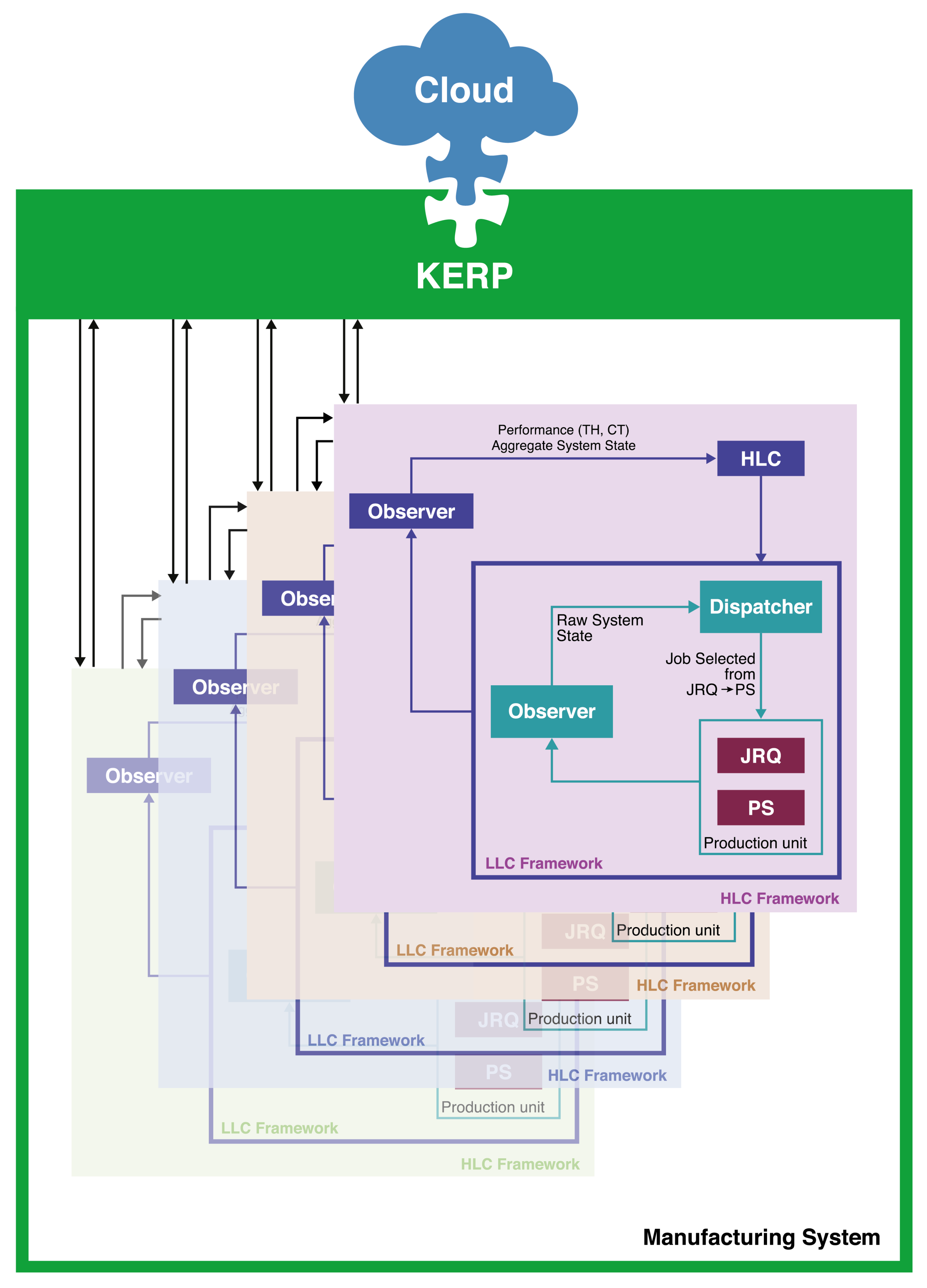
Among the most relevant scientific works, Grassi et al. [22] proposes an innovative framework of a semi-heterarchical MPC architecture distinguishing three functional levels: (i) knowledge-based enterprise resource planning (KERP), responsible for strategic operation of the system and also interacting on a cloud manufacturing base; (ii) the high-level controller (HLC), accountable for the overall performance of the supervised production system; and (iii) the low-level controller (LLC), at which the final schedule of a production unit takes place (Figure 1). As it is possible to note, the KERP level focuses on a business target (i.e., to make a profit), which translates into throughput and cycle time goals that must be met by the supervised HLCs, whereas the LLC level has a more operational goal, managing short-term scheduling activity [24]. The HLC, in particular, operates with a direct work-in-progress (WIP) control, since Spearman et al. [25] demonstrated that it is the most reliable way to be adopted for production control to ensure the achievement of expected performance targets. The perspective here is reversed with respect to the traditional MRP approach, in which orders are released with a “push” logic based on throughput estimation, and the WIP is simply an observable result.

The WIP sizing problem has already been addressed in the scientific literature, however it has only been solved in closed form for problems with restrictive assumption about processing time and production line configuration (i.e., mostly flow-shop) Hopp and Roof [26], Reyes Levalle et al. [27]. Other researchers, instead, tackled the WIP sizing problem with the application of the traditional control theory in a dynamic way [28,29,30,31]. Among these, Vespoli et al. [32] proposed a first implementation of the aforementioned semi-heterarchical architecture for Spearman et al. [25]’s controlled work-in-progress (CONWIP) flow-shop production line, taking advantage of the availability of closed form analytical models. With the aim of controlling the throughput of the supervised production line, they proposed the use of a “cascade control algorithm, composed of an optimal control law based on the analytical model from Hopp and Spearman [33], and of a secondary Proportional-Integral-Derivative (PID) controller capable of performing an additional control action that addresses the error raised by the analytical model” [34]. The proposed mechanism performs well when dealing with productive scenarios in which the assumptions at the base of the analytical model are met. However, when dealing with scenarios whose assumptions deviate significantly from the Hopp and Spearman [33]’s model ones, the proposed cascade control algorithm does not show the same promptness in setting the right level of WIP.

To improve the promptness of Vespoli et al. [32]’s throughput control and to provide a valid and reactive performance prediction tool at the higher levels of similar hybrid architectures where WIP sizing is a fundamental control lever, a model capable of predicting production performance (throughput and cycle time) with more generalized assumptions is required. The development of such a model is the main focus and contribution of this paper, ultimately providing a robust and flexible generalized solution for managing variability in mass customization scenarios.

Given the availability of analytical models in the literature, we begin by focusing on the CONWIP controlled flow-shop line formed by single-machine stations, while developments for more complex shop systems (i.e., hybrid flow-shop, job shop) are left for further research. In particular, we will initially concentrate on a balanced production line in which the only variability entering the system is related to job processing times. Starting with the most well-known analytical model available, which considers a memoryless stochastic system, a first generalization model to be used in production scenarios where processing times are generally distributed is developed. Due to the impossibility of obtaining a closed form analytical solution under the given assumptions, a machine learning procedure to be trained on simulated data [35,36] is introduced. As such algorithms perform best when trained on unrelated datasets and to allow a more generalized training, a first study was conducted to develop and validate a normalization approach, thereby enabling a one-time training on a larger dataset. Then, after demonstrating the development process of a deep learning algorithm for the given balanced CONWIP production line, the more complex problem of unbalanced production lines is considered. To that end, through the analysis of several unbalanced production lines, it was revealed that obtaining a good approximation of production performance is possible by fixing certain summations, thereby reducing the information required to describe the production line’s unbalancing. This finding has significant practical implications when using machine learning algorithms for performance prediction and optimization.

The remainder of the paper is organized as follows. Section 2 presents the theoretical background and the problem statement. Section 3 discusses the normalization approach for the throughput prediction, while Section 4 introduces the proposed machine learning algorithm for throughput estimation, comparing the results to the best mathematical model available in the literature. Section 5 extends the discussion to the unbalanced line case, and, finally, Section 6 concludes the work.

2. Theoretical Background and Problem Statement

As mentioned in the previous Section, the upcoming interest in the hybrid MPC architecture, where the WIP level of a supervised production line is a control lever to be dynamically sized, requires the development of a model capable of dynamically evaluating performances in terms of throughput and cycle time. Hence, as outlined in the Introduction section, we will focus on a flow-shop line controlled by a CONWIP control mechanism whose stations are formed by single machines with a single routing through which all processed components flow. In addition, the components (i.e., jobs or WIP) can be considered units representative of processing batches that can be reasonably measured (i.e., number of jobs or parts being processed in the line). We will therefore focus on a single-product, single-routing production line in which the only variability entering in the system is related to job processing times (Figure 2).

In this context, our research aims to answer the following research questions (RQs):

RQ1

How could a model be developed to accurately predict the performance of a CONWIP-controlled flow-shop system with generalized processing time variability?

RQ2

How can the performance of flow-shop balanced lines be effectively normalized to facilitate the training of machine learning algorithms in a single instance?

RQ3

How will the proposed model be expanded to accommodate unbalanced production line scenarios?

For the purpose of generalizing the generation of processing times, a gamma distribution with shape parameter $\alpha$ and scale parameter $\beta$ was chosen. The choice of the gamma distribution is not accidental, as it is a distribution in which the level of variability can be controlled by modulating $\alpha$. It is, in fact, a continuous probability distribution that includes the exponential distribution as a special case (when $\alpha =1$), allowing to model a variability greater than the exponential one when $\alpha <1$ and less than the exponential one when $\alpha >1$. Thanks to the flexibility of the gamma distribution, high variability scenarios (i.e., the ones related to customized production) as well as low variability ones (i.e., the ones related to standardized production) will be easily modeled.

From a modeling point of view, the CONWIP system can be conceptually reduced to a closed-loop system in which jobs never leave the production system itself, but circulate in it indefinitely in time. While the job entering the production line and the job leaving it are obviously distinct, what remains cyclical is the WIP control card that, once released, returns at the beginning of the line allowing a new job to enter [33].

Nevertheless, for this control to be consistent, mathematical models able to relate throughput (TH) and cycle time (CT) (i.e., the dependent variables) to the WIP (i.e., the independent one) are needed. In this regard, Hopp and Spearman propose three models that are valid under well-defined production conditions: best case (i.e., the best possible operating condition), worst case (i.e., the worst possible operating condition), and practical worst case (i.e., where the operating conditions admit a wide variability). These three scenarios, whose formulas are summarized in

Table 1. The performances models for single-routing and single-product CONWIP line [33].

Scenario	Cycle Time (CT)	Throughput (TH)
Best Case	$C{T}_{min}=\left\{\begin{array}{cc}{T}_0,\hfill & \mathrm{if}w\le W_0\hfill \\ \frac{w}{r_b},\hfill & \mathrm{otherwise}\hfill \end{array}\right.$	$T{H}_{max}=\left\{\begin{array}{cc}\frac{w}{T_0},\hfill & \mathrm{if}w\le W_0\hfill \\ r_b,\hfill & \mathrm{otherwise}\hfill \end{array}\right.$
Worst Case	$C{T}_{max}=w·T_0$	$T{H}_{min}=\frac{1}{T_0}$
Practical Worst Case	$C{T}_{PWC}=T_0+\frac{w-1}{r_b}$	$T{H}_{PWC}=\frac{w}{W_0+w-1}·r_b$

, are built based on the following parameters:

• $T_0$, as “the raw processing time of the line (the sum of the average processing times of each workstation at the steady state)”;
• $r_b$, as “the bottleneck rate of the line at the steady state”;
• $W_0$, as “the critical WIP of the line (i.e., the WIP level for which the line with a defined $T_0$ and $r_b$ achieves maximum throughput with a minimum cycle time if no variability exists in the system)”.

While the best case represents the maximum performance (i.e., absence of variability and balanced line) that can be obtained with a particular WIP value in the production system, the worst case represents its minimum possible performance. The most interesting case for this paper discussion is the practical worst case (PWC), which assumes that the line is balanced over the long term (i.e., the average processing times for all stations are the same), each station is formed by a single machine, and, most importantly, processing time variability is exponential. This choice is motivated by the fact that closed form analytical equations can be easily obtained only at the steady state when stochastic processes are “memoryless”.

Thus, while the PWC model is mathematically exact and solvable in closed form, it is only valid if the assumptions of exponential processing times and balanced line hold. Unfortunately, given the multitude of products and manufacturing operating condition, these assumptions can only serve as a reference, as the authors intended, that is, to provide a baseline against which the performance of an actual production system can be compared to. Indeed, the same authors developed an iterative model [25], based on an approximation of the mean value analysis, to obtain TH and CT estimations as a function of WIP in the more general case of unbalanced line and general variability of processing times. However, as already shown in [35], their estimation suffers from an approximation error that increases in magnitude as one moves away from the case of exponential variability and the balanced line hypotheses, because the model assumptions are no longer adequately verified.

The model proposed in Hopp and Spearman [33] can be summarized in the steps (1)–(4), with the following notation:

• $C{T}_j\left(w\right)$ = cycle time at station j with WIP level w;
• $CT\left(w\right)={\sum }_{j=1}^{n}C{T}_j\left(w\right)$ = cycle time with WIP level w;
• $TH\left(w\right)$ = throughput with WIP level w;
• $WI{P}_j\left(w\right)$ = average WIP level at station j with WIP level w.

Letting $WI{P}_j\left(0\right)=0$ and $TH\left(0\right)=0$, cycle time, throughput, and station-by-station WIP levels can be calculated iteratively as a function of the number of jobs:

$$C{T}_j\left(w\right)=\frac{t_e^2\left(j\right)}{2}[c_e^2\left(j\right)-1]TH(w-1)+[WI{P}_j(w-1)+1]t_e\left(j\right)$$

(1)

$$CT\left(w\right)=\sum _{j=1}^{n}C{T}_j\left(w\right)$$

(2)

$$TH\left(w\right)=\frac{w}{CT\left(w\right)}$$

(3)

$$WI{P}_j\left(w\right)=TH\left(w\right)·C{T}_j\left(w\right)$$

(4)

In light of the research questions posed, the scientific methodology for this study is structured as follows:

• Develop a simulation tool capable of generating data for the analyzed CONWIP flow-shop production system, ensuring the ability to capture the effect of generalized variability in processing times on the performances indicators (throughput and cycle time).
• Conduct a preliminary study to develop and validate a normalization approach for the performance of flow-shop balanced lines, thereby enabling one-time training on a larger dataset and facilitating the use of machine learning algorithms.
• Propose an artificial-intelligence-based model able to estimate line throughput at the steady-state, taking into account characteristic parameters and the WIP under processing.
• Demonstrate the development process of a deep learning algorithm tailored for the balanced CONWIP production line scenario, showcasing its applicability and accuracy.
• Address the more complex issue of unbalanced production lines by introducing a new index capable of identifying unbalanced situations in a way that enables the proposed model to be applied to a wider variety of production line scenarios.

This methodology aims to provide a comprehensive solution for the performance estimation of CONWIP-controlled flow-shop systems in various production environments, ultimately contributing to the development of more efficient and adaptable manufacturing processes. By leveraging machine learning algorithms trained on simulated data, the proposed model is expected to accurately estimate the actual performance of a CONWIP-controlled flow-shop system, dealing with generalized variability entering the system. The development and validation of a normalization approach for flow-shop balanced lines will allow for more effective training of machine learning algorithms, and the extension of the model to unbalanced production line scenarios will further enhance its applicability in a wider range of manufacturing contexts.

3. A Normalized Approach for the Throughput Prediction

As said before, the purpose of this work is to develop a model based on recent machine learning techniques able to estimate the performance (in terms of throughput and cycle time) of a CONWIP single-product, single-routing production system given the operating parameters of the production line and the WIP released in it. We consider the system at the steady-state, so it is sufficient to estimate only one of either TH or CT given that the other can be computed by Little’s law (i.e., $WIP=TH·CT$), the WIP being a controlled parameter. As a result, the discussion will now focus on throughput estimation, while the cycle time will be computed as $CT=WIP/TH$. Given these premises, the purpose of this paragraph is to determine which inputs are strictly necessary for the performance estimation model in order to minimize the size of the experimental campaign required to feed the model. In particular, focusing on the hypothesized production line, which is still assumed to be balanced in this phase, the operating parameters of the line are the following:

• The average processing time at the stations;
• A measure of the processing time’s variability (e.g., the coefficient of variation);
• The production line critical WIP (i.e., the previously defined $W_0$);
• The level of WIP released in the production line.

With regards to the processing time variability, it is worth noting that a dimensionless measure of processing time variability can be represented by the coefficient of variation, which is defined as the ratio of the processing time standard deviation over its mean. Since we are modeling processing times distribution by means of a gamma distribution function, and given that the scale parameter $\beta$ is computed as a function of the average processing time and the shape parameter $\alpha$, the coefficient of variation can be simply computed as $1/\sqrt{\alpha }$, confirming the fact that the variability depends only on $\alpha$. With regard to the critical WIP $W_0$, it can be shown that, in the case of balanced production lines, it exactly equals the number of machines (remember that single-machine stations are considered). As such, the number of machines is then a metric that unambiguously characterizes the production line. Finally, the last parameter is the level of WIP in the production line, which, as previously discussed, has a direct effect on the performances since it hinders the propagation of the disruptive effects of variability. The more WIP in the production line, the higher the throughput achieved or, in other words, the closer this is to the limiting value represented by the best case and, conversely, the longer the average cycle time required for the WIP to cross the production line. Finally, the average processing time relates to the bottleneck rate (i.e., the inverse of $r_b$) since the case of the balanced line is under consideration.

While it is widely recognized that training a machine learning algorithm, particularly neural networks, often requires a large dataset, they can still be effectively employed with moderate datasets, albeit at the cost of potentially reduced performance. In this study, we explore the possibility of removing the $r_b$ parameter from both data generation and prediction, given its multiplicative effect on the throughput value and the hope that it does not alter its dynamic behavior. Our aim is to derive models of throughput performance that are normalized with respect to the bottleneck rate $r_b$, thus only dependent on the variability of processing times and completely independent of the average value. This approach offers two key advantages: first, it reduces the need for large datasets to represent any different average processing time; second, the machine learning model, specifically the neural network, can be trained once (and deeply) on normalized data and then used for various values of average processing time while maintaining high accuracy. Although simpler machine learning methods could potentially be applied given the small errors observed in our test results, the adaptability and scalability of neural networks make them well suited for complex manufacturing scenarios.

Before proceeding to the experimental part, it is useful to note that Hopp and Spearman’s mathematical model already shows a confirmation of what stated, at least in the PWC case. Indeed, by adopting the previously showed PWC law (Table 1), by dividing both members by $r_b$, we obtain:

$$\frac{TH}{r_b}=\frac{w}{W_0+w-1}=f(w,W_0)$$

(5)

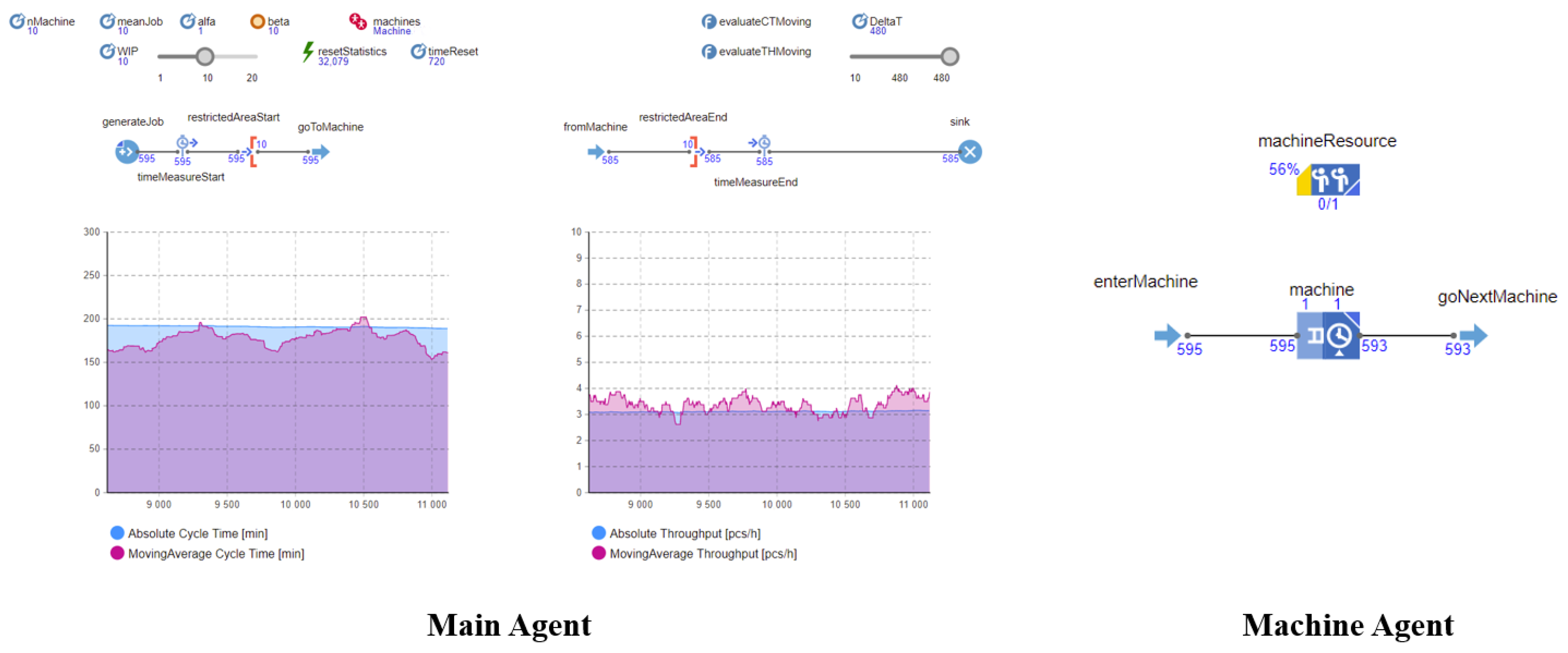
In other words, the left part represents a throughput normalized with respect to the bottleneck rate, whereas the right one is a quantity that is independent of the average processing time but dependent only on the level of WIP in the production line and on $W_0$, the critical WIP that in this balanced case is equal to the number of machines. What we expect is that, when the assumption of exponential variability is relaxed, the quantity on the right may be also dependent on the coefficient of variation, but the independence from the average processing time still remains. Due to the lack of an exact measure for these cases, a simulation tool is here used to experimentally verify if this condition is true. To accomplish this, a simulation tool capable of simulating multiple production lines in a scalable manner has been developed, taking advantages of both discrete-event and agent-based simulation techniques with the use of Anylogic simulation software.

The simulation tool is straightforward and consists of two distinct agent types: a first one, named “Main” (Figure 3), in which the CONWIP system is modeled and includes all the customization parameters necessary to characterize the various simulation scenarios; and a second one, named “Machine” (Figure 3), that consists of a service block capable of simulating both the queue of orders waiting to be processed at the machine and the waiting delay representing the processing time. The reason for developing this agent type is to create a simulator that is not only parametric in terms of average processing time, work in progress, and variability but is also able to effectively scale on the line length, measured in terms of number of machines. Finally, an automatism that can independently simulate multiple sessions (even in parallel) and save all simulation data in an Excel file in terms of performance has been developed.

The simulation tool was then validated against the previously mentioned PWC case to determine whether two-year simulation times are sufficient to achieve steady-state values of the simulated production system and whether the model is statistically representative of the theoretical performance known from the Spearman et al. [25] model, as reported in Table 1. In this regard, after evaluating the $TH$ and $CT$ for various (fixed) WIP values, a t-test was conducted to validate the results, and it was determined, with a confidence level of $99\%$ percent, that the simulation tool obtained the same average $TH$ and $CT$ values as those calculated using Spearman et al. [25]’s PWC model.

Coming back to the objective of this section, having fixed the number of machines in the single-product, single-routing line at five (it should be noted that the same conclusion may be found also when considering production lines with different number of machines), an experimental campaign was carried out according to a full factorial plan with factorial levels shown in

Table 2. Experimental factors and level for the simulation.

Experimental Factor	Level	Measure Unit
Mean processing time	$5÷50$, step 5	[min]
Shape factor ($\alpha$)	$0.5÷3$, step 0.1	[ ]
WIP level	$1÷30$, step 1	[unit]
Number of machines	5	[machines]

. Each simulation was run for a simulated time of two years, collecting the $TH$ value in terms of ratio between unit produced and the time simulated in hours (i.e., units/hours) and the normalized throughput ($TH/r_b$) which is a dimensionless number between 0 and 1. For the sake of clarity, in the following, we will refer to the normalized throughput as a percentage measure, as it may be viewed as a measure of the throughput percentage that the considered production line achieves in respect to the maximum possible throughput $r_b$.

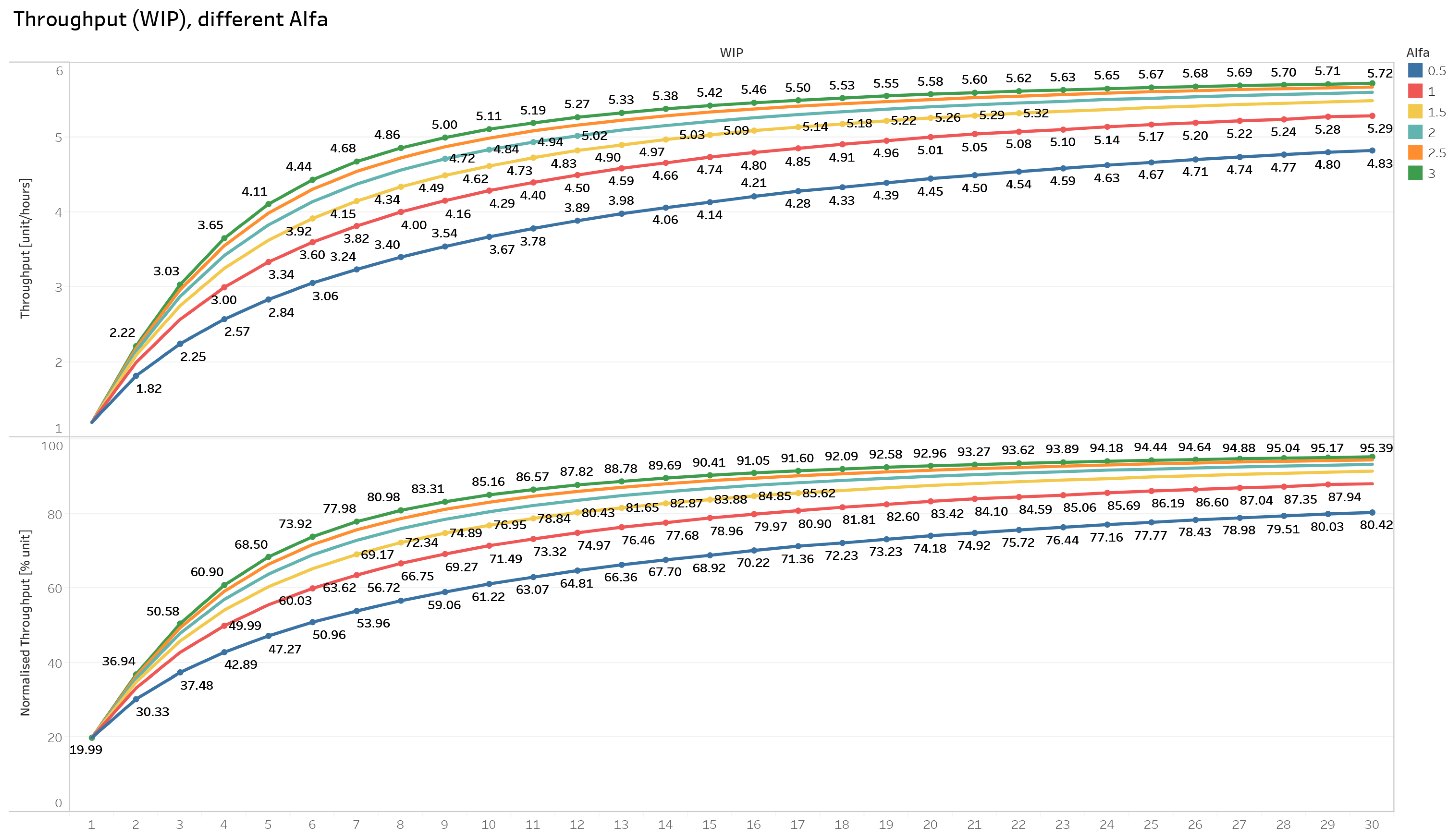
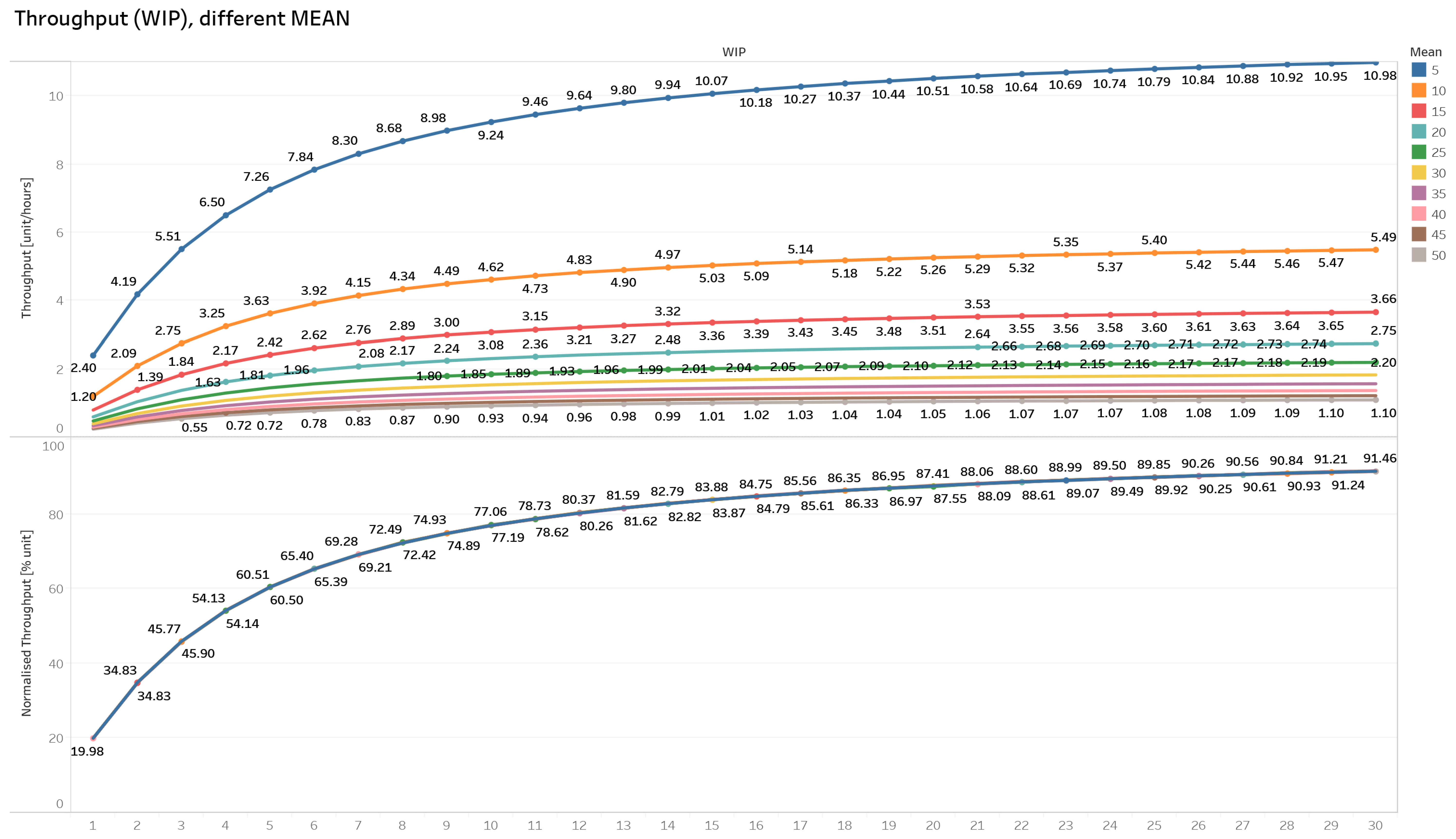
The results for the WIP values and a few of the $\alpha$ values tested are shown in Figure 4 and Figure 5 and

Table 3. The results of the simulation for a balanced CONWIP line of 5 machines.

	Alpha Value
	$\mathbf{\alpha }=\mathbf{0.5}$		$\mathbf{\alpha }=\mathbf{1}$		$\mathbf{\alpha }=\mathbf{1.5}$		$\mathbf{\alpha }=\mathbf{2}$		$\mathbf{\alpha }=\mathbf{2.5}$		$\mathbf{\alpha }=\mathbf{3}$
WIP	$\mathit{E}(\mathit{TH}/{\mathit{r}}_{\mathit{b}})$	$\Delta \%$	$\mathit{E}(\mathit{TH}/{\mathit{r}}_{\mathit{b}})$	$\Delta \%$	$\mathit{E}(\mathit{TH}/{\mathit{r}}_{\mathit{b}})$	$\Delta \%$	$\mathit{E}(\mathit{TH}/{\mathit{r}}_{\mathit{b}})$	$\Delta \%$	$\mathit{E}(\mathit{TH}/{\mathit{r}}_{\mathit{b}})$	$\Delta \%$	$\mathit{E}(\mathit{TH}/{\mathit{r}}_{\mathit{b}})$	$\Delta \%$
1	19.99	0.57%	20.00	0.31%	20.00	0.19%	20.00	0.38%	20.00	0.24%	20.00	0.14%
2	30.30	0.58%	33.34	0.18%	36.94	0.32%	35.83	0.22%	36.46	0.21%	36.94	0.15%
3	37.42	0.40%	42.86	0.25%	50.56	0.38%	47.97	0.21%	49.45	0.13%	50.56	0.11%
4	42.85	0.40%	50.02	0.29%	60.91	0.24%	57.06	0.19%	59.23	0.17%	60.91	0.10%
5	47.24	0.36%	55.55	0.26%	68.49	0.18%	63.89	0.19%	66.46	0.15%	68.49	0.18%
6	50.92	0.25%	60.00	0.19%	73.98	0.25%	69.01	0.24%	71.81	0.18%	73.98	0.15%
7	54.02	0.35%	63.64	0.19%	77.99	0.24%	73.02	0.22%	75.79	0.19%	77.99	0.16%
8	56.80	0.32%	66.66	0.24%	80.99	0.31%	76.09	0.09%	78.85	0.19%	80.99	0.16%
9	59.10	0.34%	69.23	0.13%	83.28	0.21%	78.56	0.16%	81.24	0.29%	83.28	0.11%
10	61.22	0.39%	71.42	0.32%	85.14	0.35%	80.62	0.18%	83.19	0.14%	85.14	0.13%
11	63.08	0.41%	73.35	0.21%	86.59	0.27%	82.33	0.13%	84.77	0.10%	86.59	0.08%
12	64.81	0.31%	74.99	0.25%	87.82	0.24%	83.71	0.24%	86.05	0.15%	87.82	0.12%
13	66.30	0.36%	76.46	0.31%	88.82	0.16%	84.95	0.12%	87.19	0.14%	88.82	0.12%
14	67.72	0.51%	77.79	0.32%	89.66	0.20%	86.00	0.10%	88.14	0.06%	89.66	0.15%
15	69.04	0.47%	78.97	0.16%	90.41	0.08%	86.91	0.14%	88.95	0.14%	90.41	0.16%
16	70.20	0.33%	80.03	0.36%	91.06	0.22%	87.71	0.20%	89.66	0.16%	91.06	0.12%
17	71.28	0.50%	80.92	0.29%	91.60	0.18%	88.45	0.17%	90.30	0.14%	91.60	0.12%
18	72.29	0.23%	81.81	0.31%	92.10	0.17%	89.04	0.17%	90.84	0.08%	92.10	0.09%
19	73.24	0.33%	82.59	0.16%	92.56	0.15%	89.63	0.09%	91.34	0.07%	92.56	0.11%
20	74.15	0.25%	83.35	0.23%	92.95	0.44%	90.11	0.18%	91.78	0.16%	92.95	0.12%
21	74.98	0.24%	84.02	0.35%	93.28	0.22%	90.57	0.16%	92.18	0.18%	93.28	0.16%
22	75.70	0.20%	84.62	0.39%	93.62	0.23%	90.99	0.21%	92.56	0.20%	93.62	0.13%
23	76.48	0.30%	85.17	0.30%	93.91	0.23%	91.42	0.13%	92.88	0.17%	93.91	0.09%
24	77.14	0.39%	85.69	0.39%	94.18	0.15%	91.76	0.17%	93.16	0.10%	94.18	0.19%
25	77.76	0.33%	86.23	0.15%	94.43	0.18%	92.09	0.21%	93.46	0.16%	94.43	0.13%
26	78.44	0.52%	86.65	0.18%	94.63	0.18%	92.38	0.21%	93.69	0.19%	94.63	0.09%
27	78.94	0.23%	87.07	0.18%	94.84	0.16%	92.66	0.14%	93.97	0.11%	94.84	0.24%
28	79.50	0.18%	87.50	0.38%	95.06	0.31%	92.91	0.08%	94.16	0.16%	95.06	0.17%
29	80.05	0.42%	87.90	0.20%	95.21	0.26%	93.14	0.23%	94.38	0.15%	95.21	0.10%
30	80.52	0.27%	88.25	0.28%	95.38	0.17%	93.37	0.18%	94.58	0.15%	95.38	0.18%

. In the Figure 4, the registered throughput and the normalized throughput in function of different $\alpha$ values are shown in different colors. As can be seen, the lowest curve corresponds to the smallest $\alpha$, i.e., the situation in which processing times are highly variable. On the other hand, the curves rise as the alpha value increases because, as the variability within the production system decreases, the system converges to the best case quickly as the WIP increases. A similar pattern holds true for the normalized throughput, which is clearly scaled down by a factor in comparison to the absolute throughput. On the other hand, the Figure 5 shows 10 throughput curves related to 10 different average processing times (and thus different $r_b$), with $\alpha$ set to 0.5. The highest throughput values are clearly obtained when the smallest average processing times are considered since the $r_b$ is in general a scale factor for the line throughput. Nevertheless, the curve of the normalized throughput confirms what we searched for since it practically gets values that are independent of the average processing time considered. Indeed, the different processing time curves cannot be distinguished because they are perfectly superimposed upon one on another.

To further confirm this, in Table 3, two different measures for each combination of values are reported: the average value of the normalized throughput ($E(TH/r_b)$) computed over all the observations and an error measure ($\Delta \%$) evaluated as:

$$\Delta \%=\frac{max(TH/r_b)-min(TH/r_b)}{E(TH/r_b)}·100$$

(6)

Practically, the line throughput for each of the 10 average processing times in {5, 10, 15, 20, 25, 30, 35, 40, 45, 50} was determined by executing 40 runs for each combination of $\alpha$ in $\{0.5,1,1.5,2,2.5,3\}$ and WIP in the range $[1,30]$. Then, the resulting throughput values were normalized with respect to the related $r_b$ (i.e., the inverse of the average processing time under consideration). For each combination, the maximum, minimum, and mean values were computed, and the $\Delta \%$ was calculated using Equation (6). The $\Delta \%$ represents the percentage difference between the highest and lowest observation, and the closer this value is to zero, the more similar the observations for different processing averages are one to the other, basically confirming what the considerations made about the PWC case still hold when general variability is considered. Indeed, it is useful to note that, regardless of the considered $\alpha$ value, $\Delta \%$ values remain close to zero, indicating that all observations have deviations of less than one percentage point. As a confirmation, it is worth noting that the percentage error for the various $\alpha$ is of the same order of magnitude as the percentage error for the $\alpha =1$ case, i.e., when the PWC assumptions are verified. This is significant because, in the case of an exponential distribution, the Hopp and Spearman’s mathematical model confirms the independence of the normalized throughput value from the average processing time, thus pointing out that the overall percentage deviation is due to the simulation variability and not to an unmodeled systematic error.

What has just been shown is of considerable scientific interest as it implies that, in the case of a single-product, single-routing production line that is balanced, the bottleneck rate $r_b$ acts as a scale factor for the throughput even in the general variability case. Hence, once the mean and the coefficient of variation of the processing times in the production line are known, the absolute throughput of the line at the steady state can be estimated by passing through the normalized one.

For the purposes of discussion, we can proceed with the construction of the model for predicting the throughput of a single-product line with single routing, without considering the average processing time as an input to the network and instead setting the normalized throughput as the network output. Thus, once trained, this neural network model will be able to predict the throughput of a wide variety of cases, resulting in a more generic tool.

4. The Throughput Prediction with a Deep Learning Neural Network

The goal of this paper is to take advantage of the machine learning techniques to create a deep learning neural network that, once trained, is able to identify the relationship between WIP and throughput, regardless of the degree of variability in the processing times of the jobs entering the production system. The improvement over the reference scientific literature is that, here, the model is generalized for what concerns the variability of the processing times, while maintaining the assumptions of a balanced line with controlled WIP (i.e., CONWIP), single-product and single-routing. Moreover, given what has been shown in Section 3, it will not be necessary for this neural network model to be trained over different values of the average processing times because, in the case of a balanced line, it is simply a scaling factor of the normalized throughput.

It is worth considering whether, similar to what was observed in Section 3, it might be desirable to normalize the throughput value not only in relation to the average value of the processing times but also in relation to the number of machines of the production line. Additionally, for this case, a simulation campaign has been carried out using the previously mentioned simulation tool. Differently from the previous experimental plan, here the number of machines has been varied between 5 and 15 in steps of one based on the levels of the experimental factors listed in Table 2. 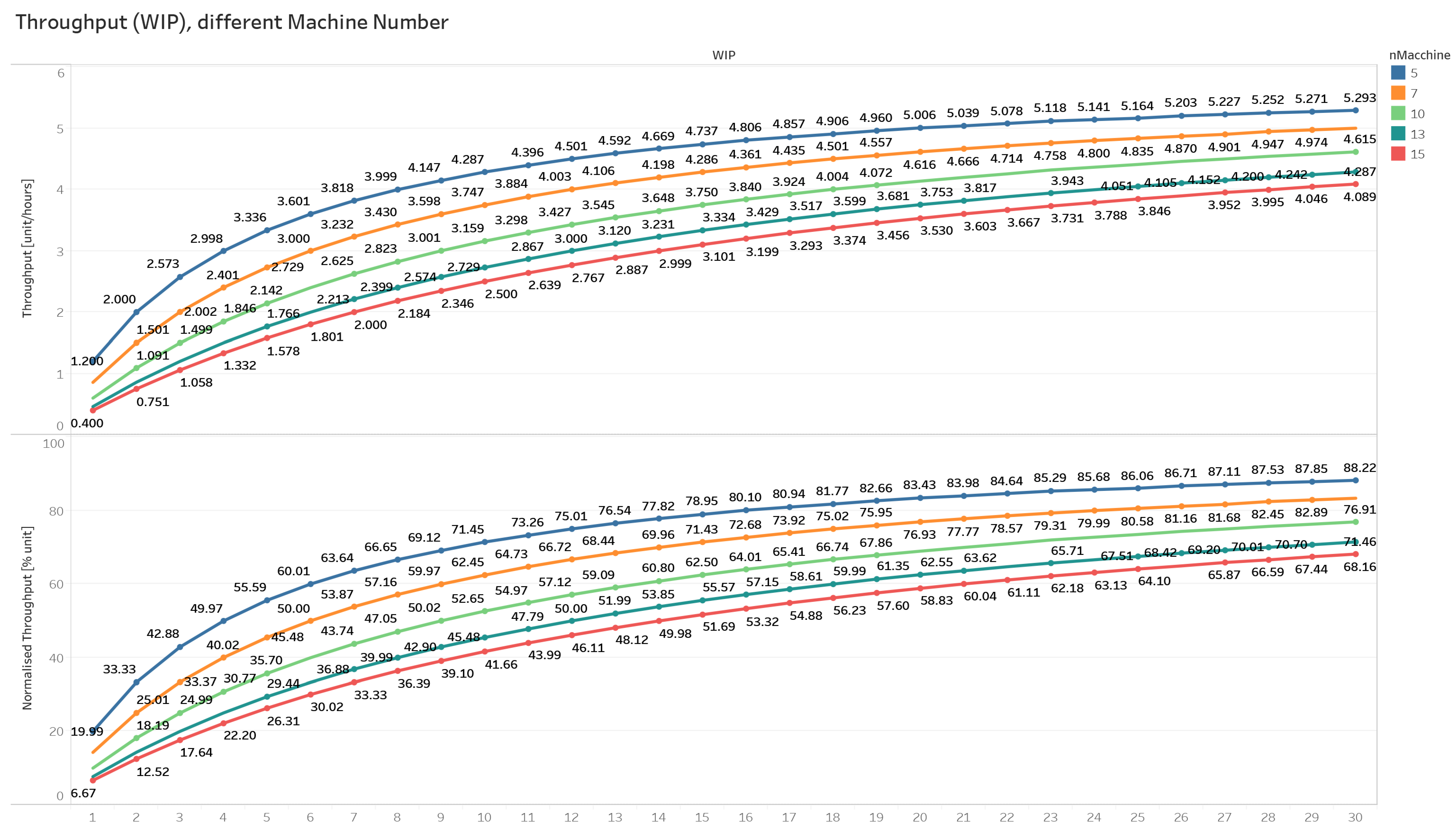Figure 5 depicts the traditional throughput and the normalized ones for a fixed value of processing times mean and coefficient of variation (i.e., fixing the alpha value of the gamma distribution). As expected, as the number of machines considered within the production line increases, both the traditionally calculated throughput and the normalized one show decreasing values (Figure 6). The bad news is that, unlike for the processing time means, this link is not as simple linear and thus cannot be easily simplified as in the first case.

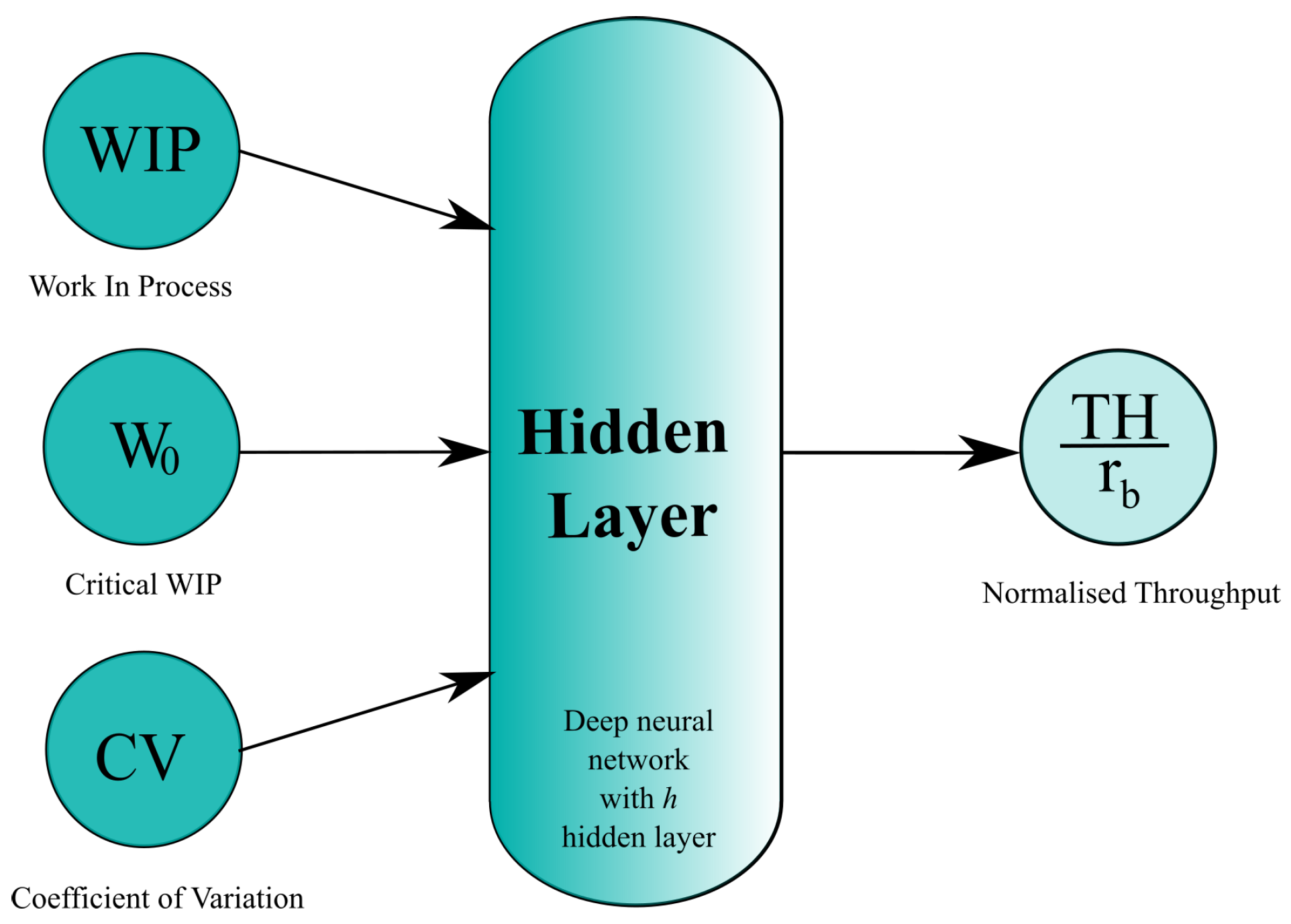
Then, the proposed deep neural network will have as inputs (i) the value of WIP released in the production line, (ii) the coefficient of variation of processing times, (iii) and the value of $W_0$ which, in the case of a balanced line, directly represents the number of machines. The output value, hence, will be the normalized throughput of the production line (see Figure 7). An intensive simulation campaign has been conducted, with the goal of providing the machine learning model with a complete dataset of the various factors under consideration. The factors and levels of experimentation involved, in particular, are those shown in

Table 4. Experimental factors and levels for the data collection.

Experimental Factor	Level	Unit of Measure
Mean processing time	$5÷50$, step 5	[min]
Shape factor ($\alpha$)	$0.5÷3$, step 0.1	[ ]
WIP level	$1÷30$, step 1	[units]
Number of machines (i.e., $W_0$)	$5÷15$, step 1	[machines]

and the experimental plan considered is full factorial. Each parameter combination was reproduced 20 times, with a simulation duration of four years of continuous manufacturing. At the end of each simulation, the absolute and normalized throughput numbers were gathered and saved in an Excel spreadsheet. More than 1,560,000 trials were conducted, yielding similar data rows that served as the dataset for the neural network training phase.

After the architecture of such a model has been determined, hyper-parameters such as the number of neurons and the structure of the hidden layer, activation functions, and loss function must be specified. However, there is no impartial way to choose these settings [37]. Consequently, these was selected with a “trial and error” technique taking advantages of Google Colaboratory and Tensor Flow Keras library for the model construction. After experimenting with various configurations, the ones that best fitted the given problem were composed of: (i) an input layer with the WIP values in the production system, the quadratic coefficient of variation and the critical WIP; (ii) a hidden normalization layer followed by 2 condensed layers of 24 neurons (12 each) with the elu and the sigmoid as activation function; (iii) a final output layer composed of a single neuron with the tanh activation function. Since the neural network is necessary to estimate the normalized throughput, which is known to range from 0 to 1, the choice of the latter activation function is not coincidental due that a value of normalized throughput larger than 1 should not be predicted.

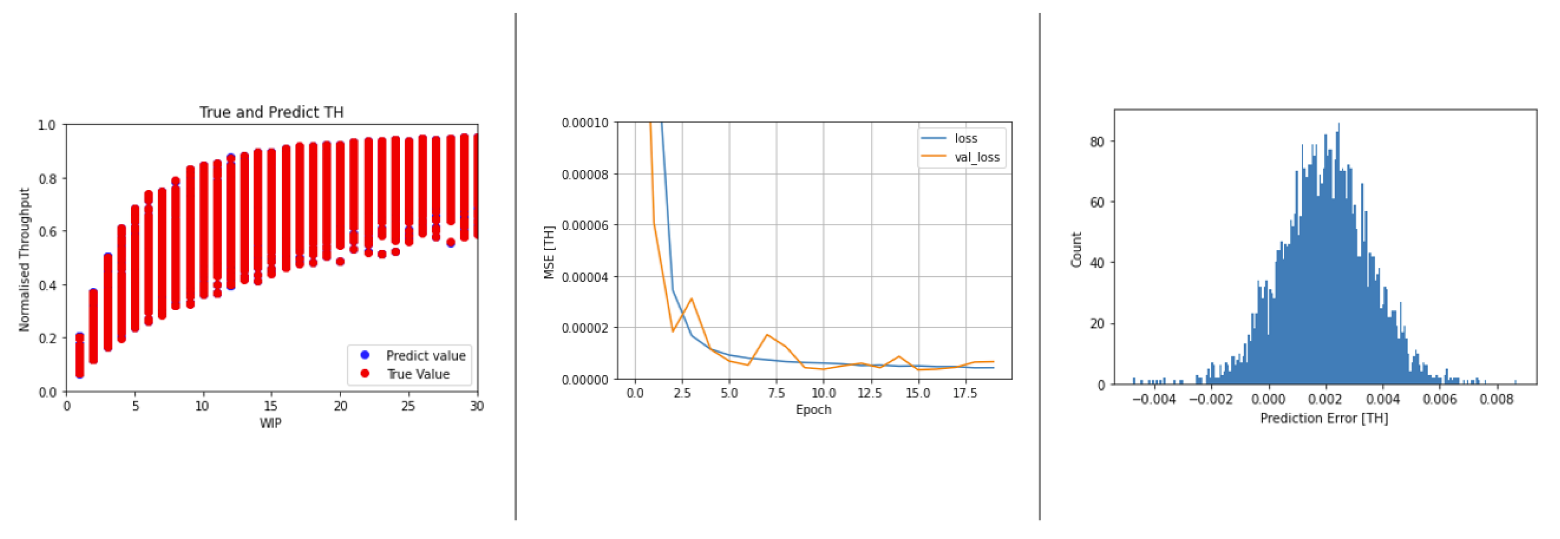
Obviously, other experiments with several neural network architectures were conducted before reaching the proposed one, which we omitted for space considerations. For the assessment of each architectures, the mean squared error (MSE) was considered as loss function. Trials with alternative learning rates were also conducted in this scenario, and the results have a satisfactory MSE value also in the test phase (MSE = $6.42\times {10}^{-6}$). For the training phase, the random seed for the initial neural net weight was fixed to guarantee an effective comparison of the outcomes, examining the model’s sensitivity to differing hyper-parameters while using the ADAM optimizer with a learning rate of 0.001. In terms of epoch number, we found that the proposed structure performed best at roughly 20 epochs, which prevented over-fitting the neural network model. Figure 8 depicts the outcomes of the deep learning neural network model.

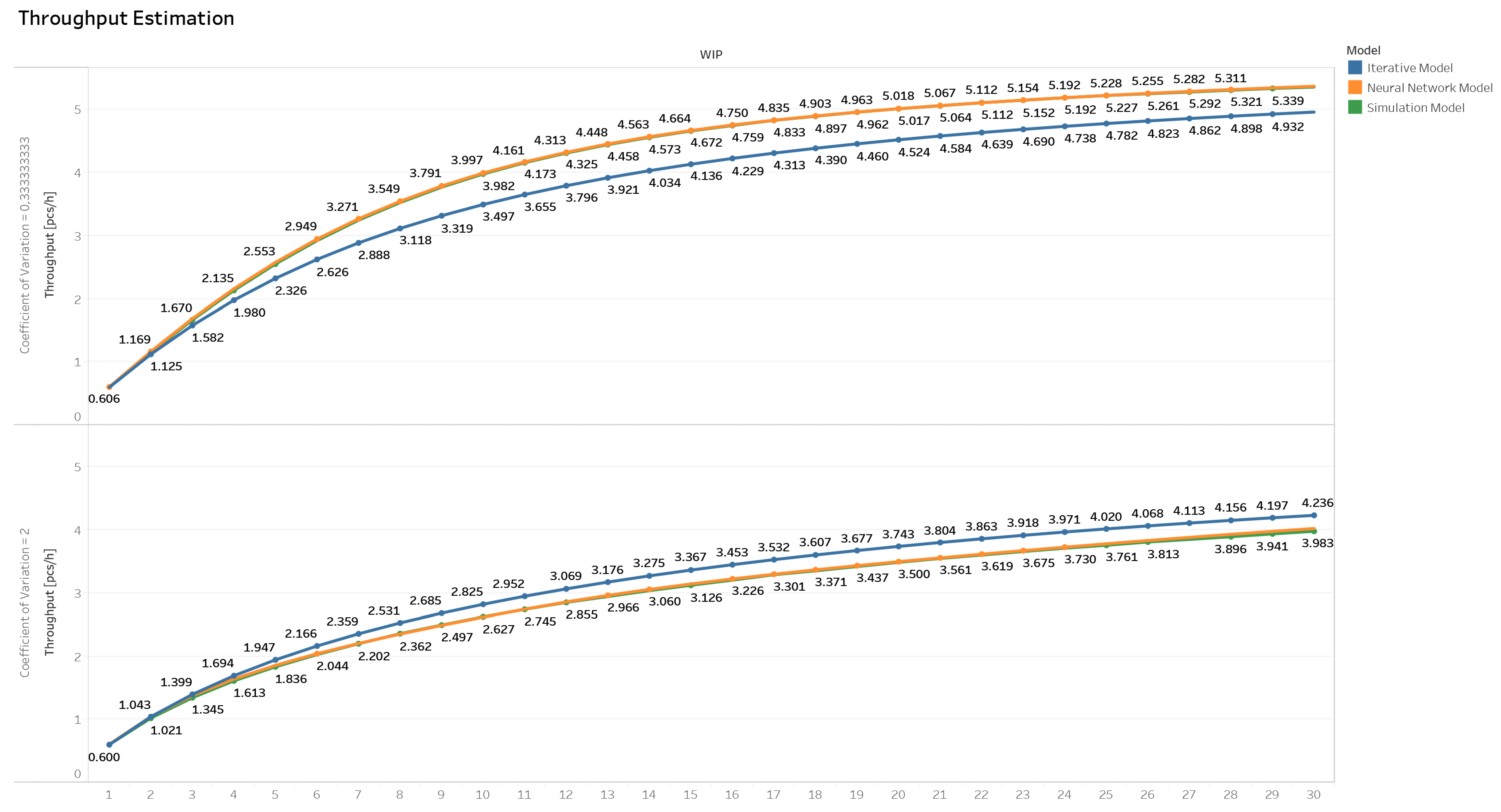
After training the model, it was subjected to a series of stress tests in which the model’s performance was evaluated under extreme or challenging conditions that deviated from the assumptions made during model development. These tests were performed for specific cases by comparing model predictions to those obtained from the simulator and Hopp and Spearman’s iterative model. It should be noted that both models produce predictions with negligible errors when the hypothesis of exponential processing times holds (i.e., when the coefficient of variation is equal to one). However, as one moves away from the exponential distribution (both for lower and higher coefficients of variation), Hopp and Spearman’s iterative model exhibits an increasing amount of drift with respect to true throughput values. In fact, without losing generality, focusing the discussion on a 10-machine scenario with average processing times set at 10 min, in Figure 9 it is possible to observe how the two models under analysis behave in the limit scenarios of the experimental plan considered (i.e., with $\alpha$ value equal to 3 and 0.5).

In the first case, when a coefficient of variation equal to 0.33 is considered, and thus a variability less than the exponential case is represented, the performance of the analyzed production system is on average better than the scenario with exponential variability. In fact, as it is possible to observe in Figure 9, the proposed neural network model (in yellow) captures the different trend completely and perfectly overlaps with the simulated values (in green), whereas the iterative model underestimates the performance (in blue). In the second case, when a coefficient of variation equal to 2 is considered, and thus a variability bigger than the exponential case is represented, the performance of the analyzed production system is on average lower than in the scenario with exponential variability. Again, the proposed model adequately captures this trend, whereas the iterative model overestimates it. This behavior is repeated for all considered cases, also where the number of machines varies, reducing in intensity when the number of machines decreases and amplifying when it increases.

In conclusion, the Hopp and Spearman’s iterative model has been shown to be very accurate for values of processing time variability close to the assumption of exponential distribution (i.e., in situations where the coefficient of variation is equal to 1) but exhibits a growing systematic error as the processing time distribution deviates from this assumption. Using an approach based on machine learning, the proposed neural network model, on the other hand, demonstrated good accuracy even in situations where processing time distribution varied substantially and to be completely generalized with respect to the average processing times, that is, normalized with respect to the bottleneck rate $r_b$.

5. Discussion on Unbalanced Lines Performance

So far, the assumption of balanced line has been considered, involving that machine processing times are taken from a distribution with the same mean value. However, in practice, this assumption is infrequently verified, as the case in which there is not a process more critical than the others is uncommon to find (i.e., there is often a process for which increasing the processing rate is costly than the others).

As a result, it is of scientific and practical interest to try relaxing the balanced line assumption. To do this, additional input parameters need to be provided to the performance estimation model. We have already shown that, from the performance estimation point of view and referring to the balanced line case, the bottleneck rate acts as a simple scale factor. Thus, we wonder if it is possible to reduce the amount of information requested to describe the unbalancing of the production line, thereby reducing the data collection and the training effort required when, as an example, a machine learning algorithm is considered. Starting from the Hopp and Spearman’s modeling approach, the production line can be generally identified by two distinct factors: the processing time of the bottleneck machine ($1/r_b$) and the average crossing time $T_0$ when queuing on machines does not occur. Letting n be the number of machines in the line, it is possible to state that the average processing time $T_0/n$ and the bottleneck processing time $1/r_b$ are unquestionably the first two mutually independent parameters to be used to identify an unbalanced production line. However, it has to be noted that they alone are not enough to express the degree of unbalancing of the line. As an example, let us consider the case of two distinct production lines with five machines that have the following distribution of average processing times:

$$\begin{array}{cc}\mathrm{Line}1:\hfill & 12;10;10;10;8\left[\min \right]\hfill \\ \mathrm{Line}2:\hfill & 12;12;11;8;7\left[\min \right]\hfill \end{array}$$

Both of the two production lines have the same raw processing time ($T_0=50$ min) and the same average processing time for the bottleneck machine ($r_b=12$ min). However, they perform significantly different in function of the WIP released. In fact, it is reasonable to expect Line 1 performing better than Line 2, owing to the fact that the first is less unbalanced than the second. This highlights the insufficiency of using only the raw processing time and the bottleneck machine processing time to distinguish between the performances of production lines with different degrees of unbalancing. In order to identify possible parameters that can uniquely distinguish production lines with the same unbalancing magnitude among stations in the production line, it is worthwhile to consider the Hopp and Spearman [25] iterative model summarized in Equations (1)–(4), which is exact in the case of a production line that is CONWIP-controlled, and the processing times are drawn from an exponential distribution. Therefore, by applying the mentioned model, it is possible to develop the iterative calculation for the throughput value (the TH formula is directly shown for reasons of space, as these can be obtained through simple mathematical steps by applying the equations iteratively):

$$\begin{gathered} TH\left(1\right)=\frac{1}{\sum \left(t\right)}=\frac{1}{T_0} \\ TH\left(2\right)=\frac{2·T_0}{\sum \left(t^2\right)+T_0^2} \\ TH\left(3\right)=\frac{3·(\sum \left(t^2\right)+T_0^2)}{2·\sum \left(t^3\right)+3·\sum \left(t^2\right)·T_0+T_0^3} \\ \dots \end{gathered}$$

As can be seen, apart from the $T_0$ value, the desired $TH\left(w\right)$ function is dependent on the sums of the processing times, where higher-order summations appear as one proceeds with the estimation of consecutive terms. In the case of a balanced line, these summations become constant, collapsing into terms that are always constant except for the value of $T_0$. In fact, if the production line is balanced, the average processing time of different workstations is always equal to $1/r_b$, meaning that:

$$\begin{gathered} \sum \left(t\right)=T_0 \\ \sum \left(t^2\right)=\frac{1}{r_b^2}+\frac{1}{r_b^2}+\dots =n·\frac{1}{r_b^2}=W_0·\frac{1}{r_b^2}=\frac{T_0}{r_b} \\ \sum \left(t^3\right)=\frac{1}{r_b^3}+\frac{1}{r_b^3}+\dots =n·\frac{1}{r_b^3}=W_0·\frac{1}{r_b^3}=\frac{T_0}{r_b^2} \\ \dots \end{gathered}$$

where n is the machine number of the production line, which is equal to $W_0$ for the balanced production line. This explains why the PWC model has such a simple and effective form since the sum of the processing times collapses in calculations dependent always on $T_0$ and $r_b$. In the case of an unbalanced line, these terms vary as the imbalance of the machines becomes more pronounced. It is of interest to investigate whether these summations are related to each other, i.e., whether fixing a sufficient number of them, the others cannot vary anymore.

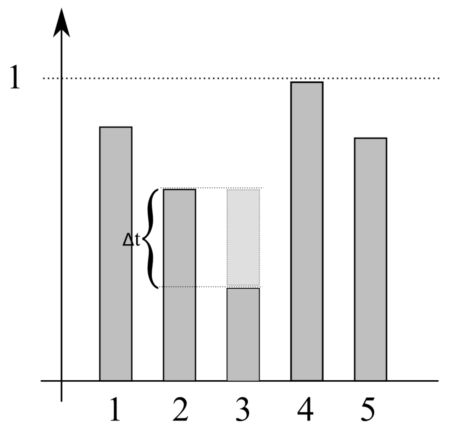
Without loss of generality, let us consider the case of a production line with five machines and analyze what happens if a defined amount of average processing time ($\Delta t$) is taken from one machine to another, without altering the $T_0$ and the $r_b$ of the considered line, as shown in Figure 10. This scenario is equivalent to the two machines swapping places, and the summations of processing time indeed remain constant in both cases. This observation confirms what the commutative property of addition would suggest that when the order of processing time sum is changed (whether they are squares, cubes, or otherwise), the result of their sum remains unaltered. In fact, as the considered production line constitutes a closed queue network (CONWIP), the position of the unbalanced production machine does not affect performance variations.

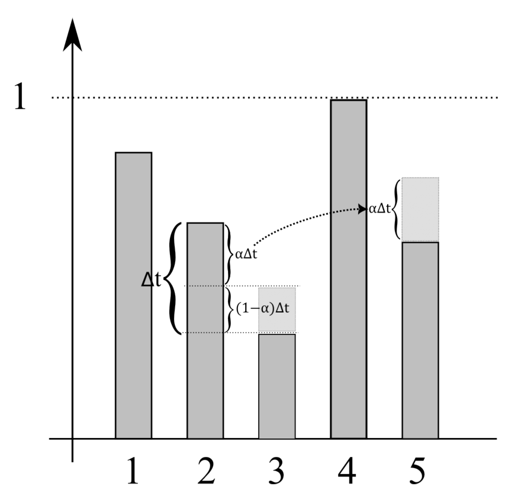
Now, consider the case of distributing the same amount of average processing time $\Delta t$ not to a single machine but dividing this amount between two other machines. In this scenario, it is possible to state that a fraction of this $\Delta t$, denoted as $\alpha$, will be assigned to one machine and the $1-\alpha$ to another. This situation is illustrated in Figure 11, in which the fraction of average processing time $\Delta t$ of machine 2 is assigned to machines 3 and 5, determining:

$$\begin{gathered} t_{2_n}=t_{2_o}-\Delta t \\ {t}_{3_n}=t_{3_o}+(1-\alpha )·\Delta t \\ {t}_{5_n}=t_{5_o}+\alpha ·\Delta t \end{gathered}$$

where $t_{m_n}$ represents the new average processing time of the m-th machine, and $t_{m_o}$ denotes the previous average processing time. It is of interest to investigate whether there exist combinations of $\alpha$ and $\Delta t$ for which the $\sum \left(t_o^3\right)$ remains unchanged for $\sum \left(t_n^3\right)$, in order to analyze the change of these solutions for the other summation terms. Considering the position of the equations above, it is possible to write:

$$\begin{gathered} \sum \left(t_n^3\right)=\sum \left(t_o^3\right)\Rightarrow \sum \left(t_n^3\right)-\sum \left(t_o^3\right)=0\Rightarrow \\ {(t_{2_o}-\Delta t)}^3+{(t_{3_o}+(1-\alpha )·\Delta t)}^3+(t_{5_o}+\alpha ·\Delta t)-(t_{2_o}^3+t_{3_o}^3+t_{5_o}^3)=0 \end{gathered}$$

Solving for $\Delta t$ yields:

$$\Delta t=\frac{t_{2_o}+t_{3_o}(\alpha -1)-t_{5_o}\alpha }{{\alpha }^2-\alpha +1}$$

(7)

Equation (7) highlights the relationship between $\Delta t$ and $\alpha$, providing a means to explore various scenarios where the redistribution of processing time does not impact the cubic summation of processing times. By analyzing these combinations, further insights can be gained into the behavior of the system under different redistributions and their effects on other performance metrics. We solved the Equation (7) numerically, showing that the only combinations that satisfy the equation are those where the amount of processing time involved in the exchange results in a situation where the machines have moved positions. For example, the actual processing time of machine $t_2$ is moved to machine $t_3$, and the processing time of machine $t_3$ to machine $t_5$. Having demonstrated this phenomenon in the case of two machines and in the case of three machines, we can inductively state that this reasoning is valid for other combinations of time shifting, always considering the case of production lines whose summation of average processing times remains constant, with a fixed $T_0$. Therefore, it is possible to conclude that even a small variation in the processing time distribution leads to a consequent change in the summations and, consequently, in the performance metrics they determine.

Therefore, from the analysis of the conducted experiment with various unbalanced production lines, it can be observed that, depending on the size of the production line, a good approximation can be accepted by fixing some summations. For example, in the case of a production line with five machines, fixing the first summation, which is equivalent to fixing the raw processing time ($T_0$), and the squared summation, the production line identified, while varying slightly in the other summations, does not cause significantly different throughput performances. In the case of ten machines, it has been observed that two summations are no longer sufficient for the approximation, but by fixing the third summation, the estimation error of performances is again limited. In an inductive way, it may be concluded that, as the number of machines in the production line increases, more summations are needed to predict the production performances accurately. However, by fixing some of the summations, it is possible to obtain a good approximation of the production performances, thus reducing the amount of information needed to describe the unbalancing of the production line. This finding can be of great practical interest, especially when considering a machine learning algorithm for performance prediction and optimization.

6. Conclusions

In today’s rapidly evolving market scenario, time to market plays a crucial role in providing a competitive edge, often surpassing the importance of mere productivity. Concurrently, the demand for increased product customization necessitates a higher level of variability within the manufacturing system. In response to these challenges, this paper contributes to the advancement of hybrid MPC architectures by developing a generalized performance estimation model for CONWIP flow-shop production lines, able to improve the promptness of the throughput control and to provide a valid and reactive performance prediction tool, where WIP sizing is a fundamental control lever.

To that end, for the case where the system is balanced, a normalization approach was proposed to generalize the measure of the throughput with the final goal of developing a machine learning tool that can be trained in one shot from a large dataset (RQ2). Then, an artificial-intelligence-based model capable of estimating normalized throughput as a function of system variability and WIP in the system was designed and validated (RQ1). The results demonstrated the model’s exceptional accuracy in predicting throughput, facilitating a finer tuning of WIP than previously achievable in scenarios with non-memoryless variability. This breakthrough has the potential to significantly improve production efficiency and adaptability in the face of ever-changing market demands.

Additionally, this paper delved into the estimation of throughput for unbalanced flow-shop production lines (RQ3). Through the analysis of various unbalanced production lines, it was revealed that obtaining a good approximation of production performance is possible by fixing certain summations, thereby reducing the information required to describe the production line’s unbalancing. This insight holds substantial practical implications, particularly when considering machine learning algorithms for performance prediction and optimization.

Despite these promising findings, the study has its limitations. The methodology presented here is focused primarily on balanced lines, and further research is needed to better understand and address the complexities of unbalanced lines. Moreover, the scope of the research is limited to CONWIP flow-shop systems and does not extend to other configurations, such as hybrid flow-shop and job-shop systems.

Looking ahead, future research may explore more generalized shop configurations, such as hybrid flow-shop and job-shop systems, with the aim of extending the normalization approach to encompass these scenarios. This may involve considering factors such as the number of machines and the type and magnitude of unbalancing present in the production system. By building on the groundwork laid by this study, forthcoming research stands to further advance the field of manufacturing, ultimately contributing to more efficient and adaptable production systems in an era of ever-increasing customization and complexity.