An Effective Plant Recognition Method with Feature Recalibration of Multiple Pretrained CNN and Layers

Abstract

Current existing methods are either not very discriminative or too complex. In this work, an effective and very simple plant recognition method is proposed. The main innovations of our method are threefold. (1) The feature maps of multiple pretrained convolutional neural networks and multiple layers are extracted; the complementary information between different feature maps can be fully explored. (2) Performing spatial and channel feature recalibration on each feature map enables our method to highlight salient visual content and reduce non-salient content; as a result, more informative features can be discerned. (3) In contrast to conventional transfer learning with end-to-end network parameters fine-tuning, in our method one forward process is enough to extract discriminative features. All recalibrated features are concatenated to form the plant leaf representation, which is fed into a linear support vector machine classifier for recognition. Extensive experiments are carried out on eight representative plant databases, yielding outstanding recognition accuracies, which demonstrates the effectiveness and superiority of our method obviously. Moreover, the retrieval experiments show our method can offer higher or competitive mean average precisions compared with state-of-the-art method. The feature visualization shows our learned features have excellent intra-class similarity and inter-class diversity for leaf species from the same genus.

1. Introduction

Plants can be seen everywhere in our daily life, such as soybeans, maple leaves, grasses and vegetables. We can get abundant resources from plants, for instance, vitamins, energy, medicines, protein, fiber and oxygen. It is estimated that there are about 400,000 plant species [1] in existence in the world, and there is a certain percentage of plants that we do not recognize adequately. According to recent research [2], human beings cause more than two kinds of plants to disappear from the earth every year on average. Hence, it is urgent to study and protect plants, which is beneficial to plant rediscovery, rare plant conservation and environment protection. The most critical and important step in protecting plants is identifying them. Additionally, once we have an accurate plant recognition software in our mobile phones [3,4], we can recognize and learn more about plants anytime and anywhere; this could further raise public awareness of plant protection. Consequently, plant recognition [5,6] is a significant research topic.

It is noteworthy that the most popular trait used for plant recognition is leaf; however, there are also many works that use other traits to accomplish plant identification and perception. Kritsis established a new dataset for Greek vascular plant recognition [7], in which the image trait includes leaf, flower, fruit and stem, the plant images are collected from tree, herb and fern. Xu constructed a minirhizotron image dataset for plant root architecture understanding [8]. Because leaf is the most basic and significant appearance feature for plants, we follow common plant recognition works [5] to utilize leaf images as our research object.

According to the summary and analysis, the difficulty of plant recognition comes from three aspects. Firstly, biological categorization is a hierarchical structure from coarse to fine: kingdom, phylum, class, order, family, genus and species; so the leaf species from the same genus share similar appearance; their visual differences are small. What is more, plant leaf images are always degraded by viewpoint, illumination, occlusion, resolution and other factors in the collection and imaging process, as a result, the similarity of homogeneous plant images decreases and the similarity of heterogeneous plant images increases. Thirdly, the semantic gap between leaf image visual content and the corresponding category labels is huge for computers. The above difficulties render plant recognition an open and challenging research direction. How to learn effective plant leaf representation is a long-standing pattern recognition problem.

Extracting discriminative features from leaf images has been recognized as an indispensable method to reduce the semantic gap. Over the past two decades, considerable efforts have been dedicated to learning effective leaf representation. In the literature, the existing plant recognition methods can be grouped into two categories: handcrafted feature methods and learning feature methods. In the early stage, researchers mainly developed plant features from the raw pixels, shape and texture of leaf images manually. Representative handcrafted methods are height description [3], shape context [9,10], local binary pattern and texture [11], triangle-based representation [12,13] and Fourier description [14]. Such features have the advantage of simple calculation and good performance for ordinary and unconstrained plant datasets; however, the accuracy will decrease dramatically for the plant leaf dataset collected in uncontrolled and wild environment.

Learning features in a data-driven fashion is gradually becoming the mainstream method of improving feature generalization abilities. Wang et al. proposed bag of fragment to discern middle-level shape features in the bag of visual words framework [15]. Zeng et al. presented a robust plant leaf identification method via locality constrained dictionary learning and sparse representation [16].

In recent years, with the renaissance of artificial intelligence technology, deep convolutional neural networks (CNN) has become one of the most important and popular technologies for computer vision tasks. CNN models have also been introduced in plant recognition [17,18,19,20], achieving great progress in classification and retrieval accuracy. It should be pointed out that the obvious disadvantage of the neural network is that it requires a large amount of learning data, a powerful computing platform and sophisticated training skills.

1.1. Motivations

Deep neural network (DNN) has been recognized as a feasible way to overcome the drawbacks of handcrafted methods in enhancing feature discrimination. However, when the sample number in an image dataset is limited, for instance, there are only 1125 and 1907 leaf images in the Swedish and Flavia datasets, training a deep convolution network from scratch is not a preferred choice, because the overfitting issue will occur definitely. Fortunately, transfer learning provides a solution to avoid the overfitting problem; however, the retraining or fine-tuning (FT) process also requires a large computational burden and sophisticated transfer experience and tricks.

Moreover, the past four years have witnessed the prosperity of attention mechanism [21] in computer vision, which learns an attention map, that is, a weight matrix or tensor, to rearrange the feature map, aiming to improve the model’s capability. The squeeze-and-excitation network learns global channel attention weight to obtain more informative features [22], which has become a plug-and-play module. We can observe and summarize that rearranging the features in a feature map via attention weight may be a plausible way to enhance discrimination ability.

In addition, different features can be learned by different CNNs, and with the deepening of the network layer, the level of learned features is gradually growing: from low-level to mid-level to high-level. Generally speaking, there always exist complementary elements between different levels of features; therefore, fusing them could improve the representation power of leaf image features.

Motivated by the analysis above, in this paper, we propose a novel method to learn features for plant leaf images, where the feature maps from multiple pretrained CNNs and multiple layers are adopted directly without the need of parameter fine-tuning; the spatial weighting and channel weighting are used to recalibrate the features without any parameter training. The feature distribution in two-dimensional space for 600 leaves from 9 species of the same genus Acer is shown in Figure 1. Although they belong to the same genus and have similar appearance, the features learned via our method for leaves from the same species are gathered closely, and the learned features for leaves from diverse species are separated clearly. This can reveal that our learned leaf features have strong discriminative power.

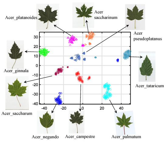
Figure 1. Our learned feature distribution of the 9 species belonging to the same genus Acer from MEW2012 dataset. The t-SNE technology is applied for feature distribution display. Images of the same class are marked with the same color and marker. A total of 600 images are used.

1.2. Contributions

The major contributions of this paper are summarized as follows:

• We present a novel feature learning method for plant leaf representation, which can exploit pretrained neural network features without time-consuming end-to-end retraining.
• We recalibrate each leaf feature map by using spatial weighting and channel weighting, which is able to capture salient information and squash non-salient information.
• We propose to leverage the feature maps of multiple pretrained CNNs and multi-layers; this strategy not only can combine the features from different networks, but also can explore the complementary elements between low-level and high-level features from different layers.
• Extensive plant leaf recognition and retrieval experiments are conducted on eight popular and complicated datasets; the mean accuracies and mean average precisions can corroborate the effectiveness and feature discrimination of our method.

The remainder of this paper is arranged as follows. Four kinds of related works are presented in Section 2. The three procedures of our proposed method are detailed in Section 3. Plant recognition experiments on eight datasets are provided in Section 4, as well as plant leaf retrieval experiments. Finally, the conclusions are presented in Section 5.

2. Related Works

2.1. Handcrafted Plant Features

Shape is one of the natural features for plant leaves; therefore, a large number of methods have been proposed to extract features from shape, for instance, shape context (SC) [9] and inner-distance shape context (IDSC) [10], where dynamic programming (DP) is applied in the shape matching stage. Adamek and O’Connor introduced capturing the contour convexities and concavities at multiple scale levels (MCC) for nonrigid shapes [23]. Hu et al. proposed a rotation, scaling and translation invariant shape contour descriptor dubbed multiscale distance matrix (MDM) [24]. It can be observed that the triangles between the shape corners have the ability to distinguish plant leaf images; therefore, a number of triangle-based methods were proposed subsequently; representative ones are triangle-area representation (TAR) [12], multiscale triangular centroid distance (MTCD) [13], triangular-based multiscale Fourier descriptor (MFD) [14] and improved multiscale triangle representation (IMTR) [25]. Texture is also an important features for plant leaves and the local binary pattern (LBP) [11] is well known as a texture descriptor. Consequently, Wang et al. proposed convoluting the leaf image with elliptical half Gabor filters and extracting the line texture features named maximum gap local line direction pattern (MGLLDP) [26]. Yang combined multiscale triangle descriptor (MTD) and local binary pattern histogram Fourier (LBP-HF) [27]; the former is used to capture the shape feature and the latter is used to characterize the texture feature. Lv et al. proposed extracting mixed multiple neighbourhood weighted LBP (MMNLBP) [28] features from different image regions. Moreover, Wang et al. proposed a novel method termed multiscale arch height (MARCH) [3] for leaf image representation, which possesses good properties of invariance, compactness and high efficiency.

2.2. Neural Network-Based Plant Features

Due to the hierarchical abstract feature learning capability by the end-to-end training manner, deep neural network models have achieved many breakthroughs in pattern recognition, natural language processing, biology, damage diagnosis and others fields. Zhou et al. introduced a filter predefined shallow CNN face image recognition method via multi-scale principle component analysis [29]. Wang et al. recently designed a new approach [30] via deep neural network and discrete cosine transform for the task of image encryption [31,32]. Yu et al. established a novel 2D CNN method via improved bird swarm algorithm [33] to evaluate the torsional capacity of reinforced concrete beams, achieving high accurate prediction results. In the community of damage diagnosis, Yu et al. [34] proposed an original method via deep stacked autoencoders to learn features for the data from multiple sensors, yielding higher diagnostic accuracy for concrete jack arch beam.

Considering the surprising progress made by neural networks in many such communities, numerous researchers also introduced neural network models to study plant image recognition. The pioneering deep learning-based plant recognition was studied in [17], where the auto-encoder and CNN were exploited to extract leaf features. Lee et al. proposed a novel plant identification method dubbed Deep Plant, which exploits CNN to learn leaf features from the raw input data and utilises deconvolutional networks to obtain insight into different orders of venation [18]. Shah et al. presented the Dual-Path CNN [19] to learn the complementation between shape and texture characteristics; their network has two branches with different kinds of inputs: leaf image and texture patch. In addition, a novel marginalized shape context descriptor was designed in [19]. To overcome the large diversity problem of plant organs, Lee et al. further proposed a hybrid generic-organ CNN (HGO-CNN) [20], in which the organ and generic information are considered and fed into two subnetworks; the features learned by the two branches are combined via a novel fusion scheme. In [35], a mask covariance network is proposed for ultra fine grained image classification, where an auxiliary self supervised learning module is devised to improve the discriminability of their model with the help of spatial covariance context of image patches. Feng leveraged radial basis kernel function [36] to extract the second-order statistics of the feature map at a specific layer of a pretrained CNN, where the principle component analysis is used to reduce channel dimensionality of the feature map. In [37], SWP-LeafNET is proposed with maximum behavioral resemblance based on botanist’s behavior, which consists of three deep learning models; two models are learned from scratch and one model is transferred from the mobile network. More recently, Wu et al. put forward the IMTD+relu5_2 [38] to study improved multi-scale triangle descriptor (IMTD) and combine the convolution features from different layers.

2.3. Transfer Learning

Transferring a CNN model pretrained on a large image dataset to other computer vision tasks is a common, effective and efficient method because it can improve the efficiency of feature learning and make full use of the learned knowledge. Ghazia et al. transferred three networks, AlexNet, VGG and GoogleNet, to plant identification [39]; in their method, data augmentation techniques, parameter fine-tuning and decision-level fusion of different classifiers are exploited to enhance overall recognition performance. Kaya et al. investigated four types of transfer learning approaches to plant classification [40], namely, VGG plus fine-tuning, VGG plus linear discriminative analysis, CNN plus recurrent neural network and AlexNet plus linear discriminative analysis. A novel nine-layer CNN is proposed to identify plant leaf disease with the help of six types of data augmentation tricks in [41], which is compared with several popular transfer learning methods. Atila et al. explored employing eight EfficientNet architectures B0–B7 and another four deep neural networks to perform a successful plant classification [42], in which all layers of the networks are set to be trainable. Different from these transfer learning methods for plant leaf or leaf disease recognition, in this paper, we directly applied pretrained CNNs to extract leaf features with only one forward process; end-to-end parameter fine-tuning is not required. Somewhat surprisingly, we found that this strategy is capable enough to achieve promising plant leaf recognition performance.

2.4. Existing Datasets for Plant Recognition

Generally speaking, there are many kinds of traits that can be used to identify plants, such as genes, fruits, leaves, flowers, plant roots and stems. Over the past several decades, biologist and image processing specialists have constructed many plant datasets to promote the development of plant recognition. Swedish [43] is a classical and simple plant dataset; there are 1125 leaves from 15 classes of trees. Flavia [44] is a collection of leaves from 32 classes of trees. The leaves in Middle European Woods (MEW) 2012 [45], CVIP100 [46] and Leafsnap [47] datasets are also gathered from trees or woods including 153, 100 and 184 species, separately. The leaf images in the ICL [3,48] dataset are captured from 220 classes of herbs and trees. The presentation forms of plants in the datasets of Oxford Flower [49] and Jena Flower [50] are various kinds of herb flowers. There are diverse root images collected from switchgrass, sesame, peanut, cotton, sunflower and papaya in the plant root minirhizotron imagery dataset [8]. The above plant databases contain single organs, such as leaves, roots and flowers. The image cross language evaluation forum (ImageCLEF) is organized for plant recognition competition; one new dataset is provided each year, containing more than one million images with different organs from trees, herbs and ferns in the PlantCLEF2015 dataset. More recently, Kritsis introduced the Greek vascular plants (GRASP) dataset [7] with 16,367 leaf, flower, fruit and stem images from 125 species that are acquired from trees, herbs and ferns.

What is more, to tackle the issue of recognizing plant diseases, numerous plant disease datasets have been established. Liu et al. constructed a large-scale plant disease dataset that has 220,592 leaf images with 271 kinds of plant disease classes [51]. Turkoglu et al. created the Turkey Plant dataset [52] to facilitate the diagnosis of diverse plant diseases and pests, consisting of 4447 unconstrained photographs from 15 categories.

3. Proposed Method

In this section, we present our method (our source code will be released at https://github.com/dxtyut/plantleaf) in detail. It is composed of three main steps: feature map extraction via multiple CNNs and layers, feature recalibration in spatial and channel dimensions, feature representation and classification. The feature extraction and recognition procedures of our proposed method are shown in Figure 2.

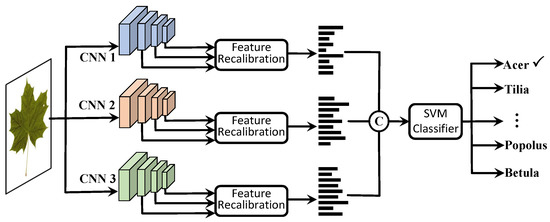
Figure 2. Our plant leaf image feature extraction and classification process.

3.1. Multiple CNNs and Layers

Since the well known residual network was proposed, for the purpose of fair comparison, the input image size of CNN- or Transformer-based models seems to be the uniform size 224 × 224 × 3. Let $\mathit{x}\in R^{a\times b\times 3}$ be a color plant leaf image; following [20], we first resize $\mathit{x}$ to make the shortest edge equal 224, then the center patch of size 224 × 224 × 3 is cropped, which is also denoted as $\mathit{x}$ in this work. We feed it into a CNN model pretrained on the large-scale image dataset imagenet [53] to extract the activated feature maps from several layers. Because there exist abundant complementary elements between low-, middle- and high-level features, we explore combining the feature maps at different layers. In addition, different CNN models distinguish plant images via learning different dominant features, so three pretrained CNN models, VGG16, VGG19 [54] and ResNet50 [55], are regarded as feature extractors with the hope of learning more discriminative cues for leaves. The features map at a specific layer L is obtained as follows:

$${\mathit{F}}_{v16}^{\left(L\right)}=VGG16(\mathit{x},L)$$

(1)

$${\mathit{F}}_{v19}^{\left(L\right)}=VGG19(\mathit{x},L)$$

(2)

$${\mathit{F}}_{res}^{\left(L\right)}=ResNet(\mathit{x},L)$$

(3)

In this paper, there are 37, 43 and 175 layers for VGG16, VGG19 and ResNet50 when the network is completely unfolded, including fully connected layers and softmax probability layer; moreover, the correlation between the convolutional features of adjacent layers is relatively strong. Therefore, in order to extract more complementation information, the activated layers of {9, 16, 23, 30} are adopted for VGG16, the activated layers of {9, 18, 27, 36} are employed for VGG19 and the activated layers of {90, 100, 110, 120, 130, 140, 152} are utilized for ResNet50.

3.2. Feature Recalibration

To simulate visual cognition in mammals, attention mechanism has been acknowledged as an indispensable module in CNN models because it can assign large weights for important features and small weights for trivial features. As shown in Figure 3, there are 24 image feature maps at one layer of ResNet for a leaf image. It is apparent that the activation responses of different channels are different, and the activation responses at different positions are also different. So recalibrating the features via attention weight is capable of highlighting discriminative features and suppressing redundant features. Most traditional attention weight matrices are fine-tuned together with the learning process of neural networks, for example, convolutional block attention module [56] and squeeze-and-excitation module [22]. For the sake of simplicity, we follow [57] in adopting a non-parametric scheme to learn the attention weight from spatial and channel dimensions.

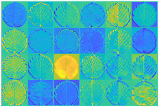
Figure 3. The first 24 feature maps of layer 15 of ResNet50 for a plant image.

Assuming the tensor shape of feature map $\mathit{F}$ at layer L is $h\times w\times c$, we compute the sum matrix $\mathit{S}$ of $\mathit{F}$ along the channel dimension as follows. The $\mathit{F}\left(c\right)$ represents the c-th channel.

$$\mathit{S}=\sum _c\mathit{F}\left(c\right)\in R^{h\times w}$$

(4)

Then the sum matrix $\mathit{S}$ is power normalized with parameter $\alpha$ and $\beta$. The spatial attention weight is calculated with the following formula:

$${\mathit{W}}_{sp}={\left(\frac{\mathit{S}}{{\left({\sum }_{x,y}{\mathit{S}}_{xy}^{\alpha }\right)}^{1/\alpha }}\right)}^{1/\beta }\in R^{h\times w}$$

(5)

where $(x,y)$ denotes the coordinate on $\mathit{S}$; the parameters $\alpha$ and $\beta$ are set to 0.5 and 2, respectively, as indicated in [57]. Finally, the weight matrix ${\mathit{W}}_{sp}$ is multiplied with each channel of $\mathit{F}$ in an element-wise manner and the resultant values are thus summed. Thereby, we obtain the spatial recalibrated features via the dot multiplication operation ⊙:

$${\mathit{f}}_{sp}={\left[\sum _{xy}{\mathit{W}}_{sp}\odot {\mathit{F}}_{xy}\left(1\right),\dots ,\sum _{xy}{\mathit{W}}_{sp}\odot {\mathit{F}}_{xy}\left(c\right)\right]}^T\in R^{c\times 1}$$

(6)

To calculate the channel weight, we firstly compute the proportion of positive numbers to the total number in each channel feature map as follows:

$$\mathsf{\Omega }=\frac{{\sum }_{xy}𝟙\left[{\mathit{F}}_{xy}>0\right]}{wh}\in R^{c\times 1}$$

(7)

where $𝟙$ is an indicator function; it returns 1 when the assertion is true and 0 otherwise. The authors in [57] found that the images from the same class have correlated channel sparsity 1-$\mathsf{\Omega }$, that is to say, channel sparsity offers discriminative information, which can be utilized to reveal the significance of infrequently occurring features. Accordingly, the channel attention weight can be calculated with the following formula:

$${\mathit{W}}_{ch}=log\left(\frac{c\delta +{\sum }_i{\mathsf{\Omega }}_i}{\delta +\mathsf{\Omega }}\right)\in R^{c\times 1}$$

(8)

where $\delta$ is a constant close to zero and is used to prevent the denominator from being zero. Finally, the weight vector ${\mathit{W}}_{ch}$ is multiplied with each position of $\mathit{F}$ in an element-wise way and all the resulting vectors are summed, so the channel recalibrated features can be obtained as follows:

$${\mathit{f}}_{ch}=\sum _{xy}{\mathit{W}}_{ch}\odot {\mathit{F}}_{xy}\in R^{c\times 1}$$

(9)

3.3. Feature Representation and Classifier

Having obtained the spatial and channel recalibrated features, we multiple them in an element-wise fashion instead of vector concatenation as follows:

$$\mathit{f}={\mathit{f}}_{sp}\odot {\mathit{f}}_{ch}\in R^{c\times 1}$$

(10)

It is obvious that one feature representation $\mathit{f}\in R^{c\times 1}$ can be deduced for each feature map $\mathit{F}\in R^{h\times w\times c}$. For the feature maps ${\mathit{F}}_{v16}^{\left(L\right)}$, ${\mathit{F}}_{v19}^{\left(L\right)}$ and ${\mathit{F}}_{res}^{\left(L\right)}$ at different layers, the corresponding recalibrated features are computed firstly and then concatenated to form the final representation of 11008 dimensionality for the leaf image $\mathit{x}$, which is followed by the $L_2$ normalization. Afterwards, in order to remove redundant features, white principle component analysis is used to reduce the feature vector’s dimensionality. In the recognition phase, the linear support vector machine (SVM) classifier is employed, in which the parameters are set to s=1 and c=10 without fine-tuning for the sake of simplicity.

In summary, the procedures of our method can be summarized as follows: (1) Split a plant leaf dataset into training set and testing set randomly. (2) Download the pretrained CNN models from the vlfeat website. (3) Extract CNN features from multiple CNNs and layers for each leaf image using MATCONVNET toolbox, where network fine-tuning is not required. (4) Call the Liblinear library to train an SVM classifier with parameter setting [-s 1 -c 10 -q]. (5) Predict the label for each test leaf image. It is worth noting that the parameters of linear SVM are not fine-tuned; we did not even try the other c and s values. We believe that the performance of our method may be enhanced if we select the optimal parameters.

4. Experiment

In this section, the necessity of multiple CNNs, multiple layers and feature recalibration are analyzed first. Extensive plant recognition experiments are then conducted on eight simple and complex plant databases in order to evaluate the effectiveness of our learned features thoroughly; the datasets are Swedish, Flavia, MEW2012, ICL, ICL compound, CVIP100, Leafsnap and Turkey Plant. The dimensionality reduction is not performed on Leafsnap and Turkey Plant. The species, training ratio and image number of train and test set are summarized in Table 1. What is more, leave-one-out test plant leaf image retrieval experiments are also carried out. The evaluation metrics are accuracy and mean average precision. Each experiment is repeated for five rounds with different training sample random selections; the average results and standard deviations are reported. The performances of our method are compared with seven handcrafted methods and nine neural network-based methods. The handcrafted methods include SC+DP [9], IDSC+DP [10], MDM [24], MTCD [13], MFD [14], MTD+LBP-HF [27] and MMNLBP [28]. The deep learning related methods are AlexNet+relu5 [58], VGG16+relu5_2 [54], Dual-Path CNN [19], Deep Plant [18], HGO-CNN [20], MaskCOV [35], KernelPool [36], SWP-LeafNET [37] and IMTD+relu5_2 [38]. The results of all the other comparative methods are quoted from the original articles or the references [3,27,38]. The software, framework and hard configuration of our implementation are MATLAB 2020a, MATCONVNET, Intel(R) Xeon(R) Silver 4210R CPU, 2.4 GHz with 64 GB. The feature extraction time for one image, the linear SVM classifier training time and the prediction time for one image are 8.89, 2.35 and 0.001 seconds, respectively. Because the leaf feature extraction processes of our method for different CNNs and different layers are independent, we believe the feature extraction time can be greatly reduced if parallel computing is applied.

Table 1. Summary of the involved plant leaf databases.

Name	Swedish	Flavia	MEW 2012	ICL	ICL Compound	CVIP100	Leaf- Snap	Turkey Plant
#Species	15	32	153	220	11	100	184	15
#Img Total	1125	1907	9745	5720	654	1208	7719	4447
Train Ratio	25	70%	30	50%	70%	70%	70%	70%
#Train Img	375	1352	4590	2860	452	807	5484	3107
#Test Img	750	555	5155	2860	202	401	2235	1340

4.1. Parameter Analysis

4.1.1. Is Feature Recalibration Necessary?

One natural question is whether the feature recalibration can improve the discriminative capability of our learned features. In order to corroborate the effectiveness of feature recalibration, we conduct several experiments on the Flavia dataset with and without feature recalibration, where nine activated layers of {16, 26, 36, 48, 58, 68, 78, 90, 100} of ResNet are used. The comparison results are shown in Figure 4; as expected, in all nine cases, our method always obtains higher recognition accuracy when the feature recalibration is applied. Therefore, we can get the conclusion that feature recalibration is a significant module in our method that can produce more informative features for leaf images.

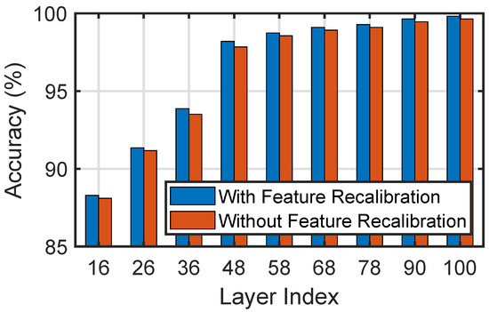
Figure 4. Recognition performance comparison of our method with and without feature recalibration on Flavia dataset under different layers of ResNet.

4.1.2. Are Multiple CNNs Necessary?

In what follows, we study the effect of multiple CNNs on the performance of our method on the Flavia dataset. The recognition results of VGG16, VGG19, ResNet and their combination are reported in Figure 5. The adopted layers for the three CNNs are {9, 16, 23, 30}, {9, 18, 27, 36} and {90, 100, 110, 120, 130, 140, 152}; each experiment is repeated five times. It can be seen that the combined model outperforms the three single models and the standard deviation of the combined model is the smallest. This indicates that a combination of multiple CNNs is an effective strategy to boost the recognition accuracy and stability for plant recognition.

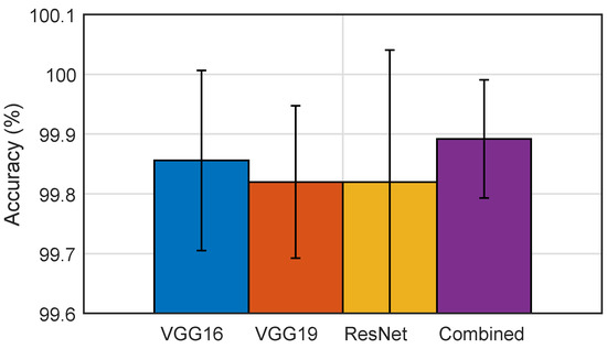
Figure 5. Comparison of recognition results between different convolution networks on the Flavia dataset.

4.1.3. Are Multiple Layers Necessary?

In this subsection, we examine the necessity of multiple layers; 19 kinds of layer configurations are studied, as shown in Table 2, which includes various types of combinations: low–low–low, low–middle, middle–high, low–middle–high, etc. The layer number ranged from 3 to 16. It should be noted again that there are 175 layers of tensors for the network ResNet50 when it is unrolled, including the prediction probability layer of size 1 × 1 × 1000. The recognition accuracy and feature length are shown in Figure 6. The greater the feature length, the higher the recognition rate generally, because more features are utilized. Obviously, one can conclude that more layers will lead to better recognition performance. Although the 9th, 12th, 14th and 15th configuration indexes obtained good enough accuracy, the 17th and 19th configuration indexes obtained higher recognition rates. Considering the trade-off between feature length and recognition rate, we select the 17th configuration index; in other words, the layers of {90, 100, 110, 120, 130, 140, 152} for ResNet are used in this work.

Table 2. Layer number configuration of ResNet used in our experiment.

# Layers	Configuration Index	Layer Configuration
3	1	16-26-36
	2	48-58-68
	3	78-90-100
	4	110-120-130
	5	140-152-162
4	6	16-26-36-48
	7	58-68-78-90
	8	100-110-120-130
	9	140-152-162-172
5	10	16-26-36-48-58
	11	68-78-90-100-110
	12	120-130-140-152-162
6	13	16-26-36-48-58-68
	14	78-90-100-110-120-130
	15	120-130-140-152-162-172
7	16	16-26-36-48-58-68-78
	17	90-100-110-120-130-140-152
	18	110-120-130-140-152-162-172
16	19	16-26-36-48-58-68-78-90-100-
		110-120-130-140-152-162-172

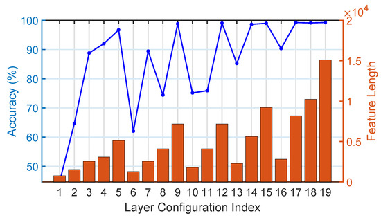
Figure 6. Accuracy and feature length for different layer configurations in Table 2.

4.2. Experiments on Swedish

Swedish is a classical and relatively simple plant leaf dataset [43], consisting of 1125 leaf images from 15 categories; each class has 75 leaves. Example images are shown in Figure 7. Following the popular train–test split scheme, for each class, 25 leaves are chosen as the training set; the other 50 leaves are used to constitute the testing set. As a result, there are 375 and 750 images in total in the training and testing set, respectively. The comparison results are enumerated in Table 3. Our method offers the highest classification rate of 99.97%, which is the average value of 100%, 100%, 99.87%, 100%, 100% for the five repeated experiments. That is to say, only one image is misclassified for the third experiment. It is evident that our learned features have strong distinguishing capability for the Swedish dataset.

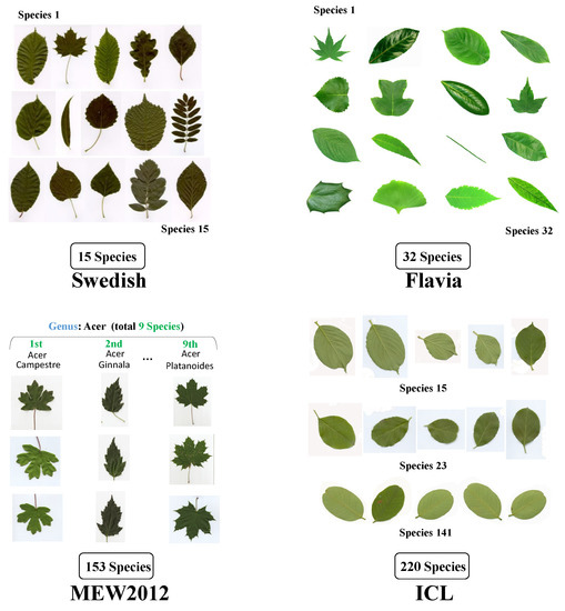
Figure 7. Example images for Swedish, Flavia, MEW2012, ICL datasets.

Table 3. Classification accuracy (%) comparison on Swedish dataset with identical settings.

Methods		Accuracy	Year
Hand	SC+DP [9]	88.12	2002 TPAMI
	MCC [23]	94.75	2004 TCSVT
	TAR [12]	95.97	2007 PR
	IDSC+DP [10]	94.13	2007 TPAMI
	MDM [24]	93.60	2012 TIP
	MARCH [3]	97.33	2015 IS
	MTCD [13]	96.31	2016 ECAI
	MGLLDP [26]	98.40	2020 ACCESS
	IMTR [25]	99.35	2020 ACCESS
	MFD [14]	97.60	2019 SPIC
	MTD+LBP-HF [27]	98.48	2021 PR
	MMNLBP [28]	99.52	2023 DSP
DNN	AlexNet+relu5 [58]	98.67	2012 NIPS
	VGG16+relu5_2 [54]	98.67	2015 ICLR
	Dual-Path CNN [19]	96.28	2017 ICIP
	Deep Plant [18]	97.54	2017 PR
	HGO-CNN [20]	96.83	2018 TIP
	MaskCOV [35]	98.27	2021 PR
	KernelPool [36]	99.87	2022 MTA
	IMTD+relu5_2 [38]	99.47	2023 ESA
	Ours	99.97(±0.06)	-

4.3. Experiments on Flavia

As illustrated in Figure 7, there are 1907 leaves from 32 plant species in the Flavia [44] dataset; the image number is about 50-70 for each species. We follow [38] to adopt the common setting: 70% images per species are selected as training images; the other 30% as testing images. There are 1352 and 555 leaf images in total in the training and testing set, respectively. The recognition results of our method and the competing methods are tabulated in Table 4. Our method achieves the highest classification rate of 99.89%, which is the average value of 100%, 99.82%, 99.82%, 100%, 99.82% for the five repeated experiments. The accuracy gain of our method over the best handcrafted MMNLBP [28] is 0.59%. The improvement of our method over the second best neural network-based method, KernelPool [36], is 0.18%. The main reasons for the superior performance of our method are twofold: complementation information utilization between various CNNs and layers; the discriminative features highlighted via feature recalibration.

Table 4. Classification accuracy (%) comparison on Flavia dataset with identical settings.

Methods		Accuracy	Year
Hand	SC+DP [9]	84.62	2002 TPAMI
	IDSC+DP [10]	77.80	2007 TPAMI
	MDM [24]	82.55	2012 TIP
	MTCD [13]	85.49	2016 ECAI
	MFD [14]	89.51	2019 SPIC
	MTD+LBP-HF [27]	99.16	2021 PR
	MMNLBP [28]	99.30	2023 DSP
DNN	AlexNet+relu5 [58]	97.60	2012 NIPS
	VGG16+relu5_2 [54]	98.25	2015 ICLR
	Dual-Path CNN [19]	99.28	2017 ICIP
	Deep Plant [18]	98.22	2017 PR
	HGO-CNN [20]	97.53	2018 TIP
	MaskCOV [35]	99.30	2021 PR
	KernelPool [36]	99.71	2022 MTA
	SWP-LeafNET [37]	99.67	2022 ESA
	IMTD+relu5_2 [38]	99.65	2023 ESA
	Ours	99.89(±0.09)	-

4.4. Experiments on MEW2012

The objective of conducting this experiment is to evaluate our method on the more complicated plant dataset, MEW2012 [45]. There are 9745 leaf images from 153 species, containing 50 to 99 leaves for each species; example images are shown in Figure 7. There are also intra-class differences and inter-class similarities caused by the variations of image scale, viewpoint, color, illumination, etc. The biggest challenge for MEW2012 is that many species come from the same genus, as shown in Figure 8. In other words, the species belonging to the same genus share similar visual appearance that renders MEW2012 a challenging plant leaf dataset. The comparison of our method and the other 14 comparative methods is displayed in Table 5. Our method obtains the highest recognition rate, 99.41%, which is the average value of 99.28%, 99.38%, 99.32%, 99.50% and 99.59% for the five repeated experiments. Our approach outperforms the best handcrafted method MTD+LBP-HF [27] by a large margin of 3.77%. The improvements of our method over the famous deep learning methods Dual-Path CNN, Deep Plant and HGO-CNN are 4.83%, 7.25% and 5.39%, respectively. Although IMTD+relu5_2 [38] combines multi-scale triangle descriptor and convolutional features, its accuracy is still inferior to our accuracy by a margin of 3.2%. Although KernelPool [36] obtains results close to our method, its feature length is larger than ours. Its outstanding performance demonstrates the superiority of our method in learning features for plant leaf recognition.

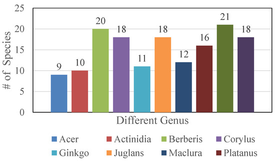
Figure 8. The species number for the 10 genera of the MEW2012 dataset.

Table 5. Classification accuracy (%) comparison on MEW2012 dataset with identical settings.

Methods		Accuracy	Year
Hand	SC+DP [9]	82.04	2002 TPAMI
	IDSC+DP [10]	71.60	2007 TPAMI
	MDM [24]	65.47	2012 TIP
	MTCD [13]	85.12	2016 ECAI
	MFD [14]	89.31	2019 SPIC
	MTD+LBP-HF [27]	95.64	2021 PR
DNN	AlexNet+relu5 [58]	96.41	2012 NIPS
	VGG16+relu5_2 [54]	98.06	2015 ICLR
	Dual-Path CNN [19]	94.58	2017 ICIP
	Deep Plant [18]	92.16	2017 PR
	HGO-CNN [20]	94.02	2018 TIP
	MaskCOV [35]	98.32	2021 PR
	KernelPool [36]	99.37	2022 MTA
	IMTD+relu5_2 [38]	99.09	2023 ESA
	Ours	99.41(±0.13)	-

4.5. Experiments on ICL

To further evaluate the potential power of our approach in plant recognition, in this experiment, we utilize the ICL dataset [3,48]; there are 16851 leaves from 220 classes; the leaf image number and species number are both more than in the MEW2012 dataset. The image number in each species ranges from 26 to 1078. The ICL dataset is constructed by the Intelligent Computing Laboratory at Hefei Botanical Garden, Hefei, Anhui province, China. From Figure 7, we can see that the visual appearance of the images from the 15th, 23rd and 141st species are very similar; this implies ICL is a more challenging dataset. We follow [3] in using the first 26 leaf images for each species and setting the training ratio to 50%; therefore, both have 2860 samples in the training set and testing set. The classification comparison results are shown in Table 6; our method achieves the best accuracy result of 98.67%, which is the mean value of 98.71%, 98.88%, 98.64%, 98.43% and 98.71% for the five repeated experiments. Compared with handcrafted features, deep neural network-based methods obtain higher classification rates because they have automatic hierarchical semantic feature learning abilities. Our method outperforms the well known handcrafted leaf descriptor MARCH [3] by a margin of 12.64%. The accuracy of our method is 11.75%, 4.09% and 0.81% higher than that of VGG16+FT, ResNet50+FT and KernelPool, which can be attributed to the usage of complementation information between the convolution features from various layers and CNNs and salient features boosted by feature recalibration in our method.

Table 6. Classification accuracy (%) comparison on ICL dataset with identical settings.

Methods	Accuracy	Year
MCC [23]	73.17	2004 TCSVT
TAR [12]	78.25	2007 PR
IDSC+DP [10]	81.39	2007 TPAMI
MARCH [3]	86.03	2015 IS
VGG16+FT [54]	86.92	2015 ICLR
ResNet50+FT [55]	94.58	2016 CVPR
KernelPool [36]	97.86	2022 MTA
Ours	98.67(±0.16)	-

4.6. Experiments on ICL Compound

According to the statistics and analysis, the images in the 10th, 12th, 25th, 27th, 49th, 56th, 126th, 132nd, 168th, 169th and 215th species of the ICL dataset are compound leaves, where a compound leaf splits several times in the middle to form two or more leaflets. Obviously, the compound leaf images bring more challenges to plant recognition. Therefore, Wang et al. [59,60] collected those leaf images to construct the ICL compound dataset; there are 11 classes and 654 leaves in total; example images are shown in Figure 9. In order to assess the effectiveness of our method on compound leaves, we conduct an experiment on the ICL compound dataset. The training ratio for each class is 70%; the remaining 30% is used for testing. As we can see from the comparison results in Table 7, our method also obtains the amazing accuracy of 100% for all the five repeated experiments, which again corroborates the effectiveness of our method in learning discriminative features for plant leaves.

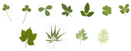
Figure 9. Example images from ICL compound dataset, one image for each species.

Table 7. Classification accuracy (%) comparison on ICL compound dataset with identical settings.

Methods		Accuracy	Year
Hand	SC+DP [9]	96.94	2002 TPAMI
	IDSC+DP [10]	94.90	2007 TPAMI
	MDM [24]	94.90	2012 TIP
	MTCD [13]	95.92	2016 ECAI
	MFD [14]	97.96	2019 SPIC
	MTD+LBP-HF [27]	100	2021 PR
DNN	AlexNet+relu5 [58]	100	2012 NIPS
	VGG16+relu5_2 [54]	100	2015 ICLR
	Dual-Path CNN [19]	98.56	2017 ICIP
	Deep Plant [18]	94.90	2017 PR
	HGO-CNN [20]	96.43	2018 TIP
	MaskCOV [35]	100	2021 PR
	IMTD+relu5_2 [38]	100	2023 ESA
	Ours	100(±0.00)	-

4.7. Experiments on CVIP100

The CVIP100 dataset [46] contains 1208 leaf images from 100 species; each class has at least 12 images. Figure 10 illustrates 24 images for 4 species; one can observe that the leaves for many species have very similar shapes, textures and visual appearance, and image rotation is also a variation factor, which makes CVIP100 a challenging plant dataset. In each category, 70% of the images are considered the training set; the rest are regarded as the testing set. The comparison results are reported in Table 8. Our proposed method achieves 99.65% recognition accuracy, which is the average value of 100%, 99.75%, 99.50%, 99.75% and 99.25% for the five repeated experiments. AlexNet+relu5 [58] and VGG16+relu5_2 [54] only utilize the features from one layer, which leads to a lack of sufficient characteristics. As a result, these methods cannot achieve an extremely promising recognition rate. Similar to the results in the previous tables, the neural network-based methods generally obtain higher results than handcrafted methods, which reveals the advantages of convolutional features. We further combine the convolutional features from multiple CNNs and multiple layers; therefore, our approach can provide higher recognition results as expected. Our method outperforms the best state-of-the-art method IMTD+relu5_2 [38] by a margin of 0.4%.

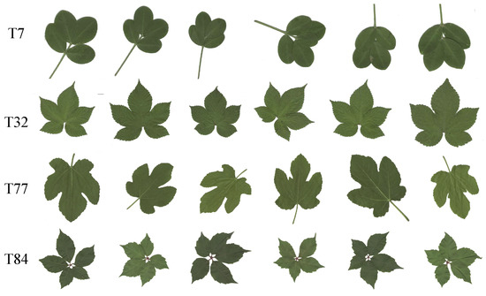
Figure 10. Example images from CVIP100 dataset; four species are shown.

Table 8. Classification accuracy (%) comparison on CVIP100 dataset with identical settings.

Methods		Accuracy	Year
Hand	SC+DP [9]	92.25	2002 TPAMI
	IDSC+DP [10]	87.75	2007 TPAMI
	MDM [24]	80.25	2012 TIP
	MTCD [13]	88.75	2016 ECAI
	MFD [14]	94.50	2019 SPIC
	MTD+LBP-HF [27]	97.50	2021 PR
DNN	AlexNet+relu5 [58]	96.00	2012 NIPS
	VGG16+relu5_2 [54]	98.20	2015 ICLR
	Dual-Path CNN [19]	95.78	2017 ICIP
	Deep Plant [18]	94.26	2017 PR
	HGO-CNN [20]	95.16	2018 TIP
	MaskCOV [35]	96.25	2021 PR
	IMTD+relu5_2 [38]	99.25	2023 ESA
	Ours	99.65(±0.28)	-

4.8. Experiments on Leafsnap

We further evaluate the performance of our method on a large-scale plant dataset Leafsnap [47]. Leafsnap includes 23147 lab images and 7719 field images from 184 tree species. The image number varies from 10 to 183 for each tree species. As shown in Figure 11, the leaf images from diverse categories have similar shape and visual appearance. Therefore, it is very challenging to distinguish the leaves in Leafsnap correctly. In our experiment, we use the field images; seventy percent of the images in each species are regarded as the training set, the other thirty percent as the testing set. All comparison results on this dataset are tabulated in Table 9. Our method achieves 93.40% recognition rate, which is the average value of 93.55%, 92.80%, 92.80%, 94.49% and 93.36% for the five repeated experiments. Because large variations existed in the leaf images of Leafsnap, the recognition accuracies of all handcrafted methods are less than 75%. Among the neural network-based methods, our proposed method outperforms the second and third best methods by 2.11% and 3.28%. The experiment results can demonstrate the effectiveness of our method evidently.

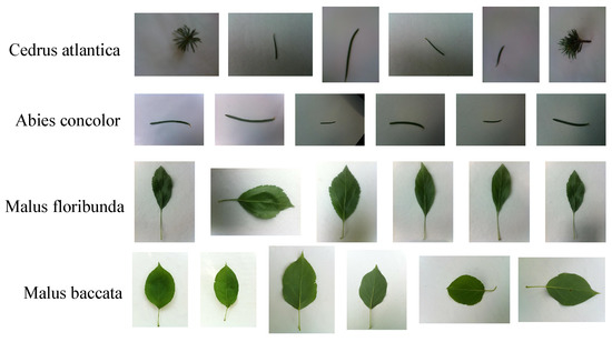
Figure 11. Example images from Leafsnap dataset; four species are shown.

Table 9. Classification accuracy (%) comparison on Leafsnap dataset with identical settings.

Methods		Accuracy	Year
Hand	SC+DP [9]	59.21	2002 TPAMI
	IDSC+DP [10]	46.81	2007 TPAMI
	MDM [24]	39.66	2012 TIP
	MTCD [13]	50.59	2016 ECAI
	MFD [14]	61.07	2019 SPIC
	MTD+LBP-HF [27]	73.65	2021 PR
DNN	AlexNet+relu5 [58]	86.61	2012 NIPS
	VGG16+relu5_2 [54]	89.86	2015 ICLR
	Dual-Path CNN [19]	88.54	2017 ICIP
	Deep Plant [18]	86.12	2017 PR
	HGO-CNN [20]	86.57	2018 TIP
	MaskCOV [35]	90.12	2021 PR
	IMTD+relu5_2 [38]	91.29	2023 ESA
	Ours	93.40(±0.69)	-

4.9. Experiments on Turkey Plant

The Turkey Plant disease and pest dataset was established by the Agricultural Faculty of Bingol and Inonu Universities in Turkey [52]; we call it Turkey Plant in this paper for the sake of simplicity. It is designed to promote the research of plant disease and pest recognition. There are 4447 images of size 4000 × 6000 from 15 categories. The minimal and maximum sample number for an image class are 69 and 1110, respectively. Example images for each class are shown in Figure 12. The image background is very complex and in each class, for example, Apple Aphis spp, some images only contain many apple leaves inside, some images contains apple fruits and leaves inside, some images focus on the tree branch and a few leaves and some images do not have leaves. Therefore, it is hard to identify different plant diseases correctly; that is to say, Turkey Plant is an extremely challenging plant disease dataset. In order to test the performance of our method on Turkey Plant, we conducted an experiment to compare our method and other competing methods, the comparison results are presented in Table 10; our proposed method achieves the highest recognition accuracy, 96.19%, which is the average value of 95.82%, 97.01%, 96.27%, 96.49% and 95.37% for the five repeated experiments. More importantly, our method is the only method with a recognition rate of more than 90%, which outperforms the second best method by nearly 10%. Compared with the results on previous plant datasets, the performance of the handcrafted methods decrease heavily; the reason is that those methods extract leaf shape information; however, it is difficult to estimate the shape features for the leaves in the Turkey Plant dataset. It is obvious that our learned plant features are very effective and discriminative for plant leaf disease recognition even if the plant images have a complex background, scale variations and viewpoint rotation.

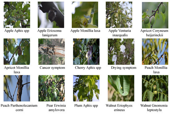
Figure 12. Example images from Turkey Plant dataset; one image for each species.

Table 10. Classification accuracy (%) comparison on Turkey Plant dataset with identical settings.

Methods		Accuracy	Year
Hand	SC+DP [9]	22.17	2002 TPAMI
	IDSC+DP [10]	19.55	2007 TPAMI
	MDM [24]	17.60	2012 TIP
	MTCD [13]	18.50	2016 ECAI
	MFD [14]	20.22	2019 SPIC
	MTD+LBP-HF [27]	28.61	2021 PR
DNN	AlexNet+relu5 [58]	80.67	2012 NIPS
	VGG16+relu5_2 [54]	86.59	2015 ICLR
	Dual-Path CNN [19]	83.56	2017 ICIP
	Deep Plant [18]	82.58	2017 PR
	HGO-CNN [20]	82.43	2018 TIP
	MaskCOV [35]	86.14	2021 PR
	IMTD+relu5_2 [38]	86.83	2023 ESA
	Ours	96.19(±0.63)	-

Moreover, we display the confusion matrix for the recognition results on Turkey Plant in Figure 13, in which $ci$ means the i-th class. Among the 15 categories, there are 12 categories with accuracy beyond 90% and 3 categories with accuracy equal to 100%. The misclassified samples of each category are 6, 2, 10, 6, 1, 3, 0, 1, 0, 4, 1, 2, 2, 0, 2 respectively. The confusion matrix can reveal that our method is robust against dataset unbalancing.

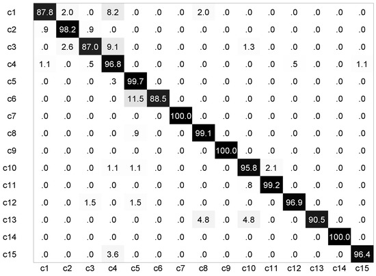
Figure 13. Confusion matrix result of our method on Turkey Plant dataset.

4.10. Leaf Retrieval Experiment

In this section, in order to evaluate the feature discriminative ability of our method further, several experiments are carried out to compute the leaf retrieval results, where the leave-one-out test scheme is applied. Suppose that there are N samples and K categories in a leaf dataset and let $X_{ki}$ be the i-th leaf image that belongs to class k with $C_k$ samples. Firstly, we compute the Euclidean distances between $X_{ki}$ and the other N-1 leaf images. Secondly, the average precision [61] for $X_{ki}$ is formulated as follows:

$$AP\left(X_{ki}\right)=\frac{{\sum }_{n=1}^{N-1}(P\left(n\right)\times s\left(n\right))}{C_k-1}$$

(11)

where $P\left(n\right)$ means the precision at cut-off n; $s\left(n\right)$ is equivalent to 1 if the n-th retrieval image is relevant to $X_{ki}$ and 0 otherwise. Finally, the retrieval evaluation metric mean average precision (MAP) can be obtained via the following equation:

$$MAP=\frac{1}{N}\sum _{k=1}^K\sum _{i=1}^{C_k}AP\left(X_{ki}\right)$$

(12)

Without loss of generality, two simple leaf datasets (Swedish, Flava) and two complicated datasets (Leafsnap, Turkey Plant) are used in our retrieval experiments. The retrieval MAP results of our method are compared with those of the newly published state-of-the-art approach IMTD+relu5_2 [38]. One can see from Figure 14 that our method gets higher MAP scores on Swedish and Turkey Plant than IMTD+relu5_2. The MAP scores of our method on Leafsnap is 49.16%, which is very close to the 49.44% of IMTD+relu5_2.

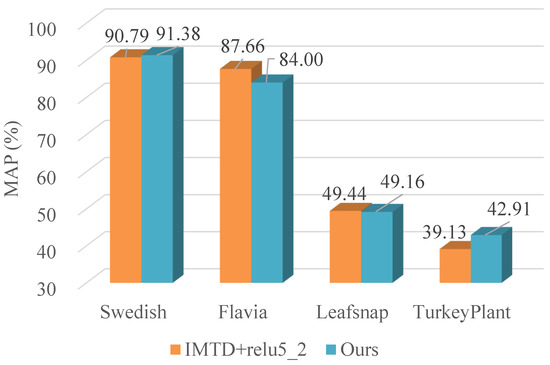
Figure 14. Retrieval MAP performance comparison between our method and the state-of-the-art method IMTD+relu5_2.

We randomly select five leaf images from Flavia dataset and display the top 10 retrieval results for each leaf image. It can be seen from line 2 of Figure 15 that there is only one wrong retrieval result that shares similar appearance with the query image. What is more, we also display the top 10 retrieval results for five leaf images from the Leafsnap datastet. The closest retrieval images for all the five queries are correct, which is consistent with the identification results in Table 9. All the 10 retrieval results are correct for the query images in lines 3 and 5 of Figure 16; this can prove the feature representation ability of our method. Although there are several wrong retrieval results in lines 1, 2 and 4 of Figure 16, the wrong retrieval leaves have visual appearance and shape very similar to the query images, especially for the results in lines 1 and 4.

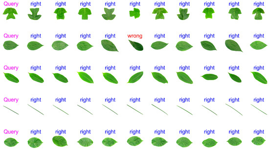
Figure 15. Top 10 retrieval images for five leaf images from Flavia dataset.

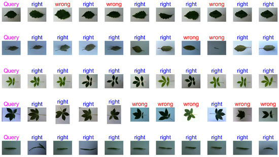
Figure 16. Top 10 retrieval images for five leaf images from Leafsnap dataset.

4.11. Effect of Classifier

In this section, we study the effect of different classifiers on the performance of our method, including LinearSVM with parameters c = 10 and s = 1, ridge regression classifier (RRC) with parameter $\lambda$ equal to 0.005, nearest neighbour classifier with cosine distance and ensemble classifier Bagging (fitensemble (data, label, ‘Bag’, 100, ‘tree’, ‘type’, ‘classification’)). For comparison fairness, each experiment is repeated for 20 rounds here. It should be emphasised that we do not optimize the parameters of the four classifiers; the usual parameter values are applied. We believe that the performance of our method could be further promoted if the parameters are fine-tuned. Without loss of generality, the two complicated datasets Leafsnap and Turkey Plant are used. From the box plot Figure 17, we can see LinearSVM yields the second best results. Surprisingly, the RRC obtains slightly better performance than LinearSVM. Even the results of nearest neighbour classifier decrease by 3–5%, but it is still promising compared with the results in Table 9 and Table 10. Bagging classifier obtains unsatisfying results; the reason is probably that the ensemble method and tree number should be chosen carefully; however, we just use the default setting.

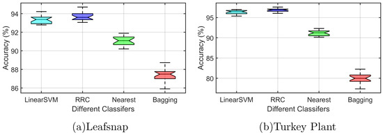
Figure 17. Recognition performance of four classifiers on two complicated datasets.

5. Conclusions

In this work, we present a novel, effective and very simple feature extraction method for plant recognition, which consists of three stages: extracting feature maps from multiple CNNs and multiple layers, feature recalibration and classification via the off-the-shelf linear support vector machine classifier. Our approach is able to take advantage of the complementation information between the layers of different CNNs. In addition, feature recalibration is capable of highlighting informative features and suppressing redundant features, which is important to image classification tasks. As a result, the feature distributions show that our learned features have excellent separating ability for the nine leaf species even from the same genus; see Figure 1. Our method can achieve leading performance on eight representative datasets compared with seven handcrafted and nine deep learning-based methods; see Table 3, Table 4, Table 5, Table 6, Table 7, Table 8, Table 9 and Table 10. Additionally, the retrieval MAP scores of our approach are better or very close to those of the state-of-the-art method; see Figure 14, Figure 15 and Figure 16. In the near future, we intend to devise vision transformer-based networks to learn plant leaf features, fusing the contrastive learning mechanism may be an effective way to enhance feature learning ability.

References

- Wang, X.; Huang, D.; Du, J.; Xu, H.; Heutte, L. Classification of plant leaf images with complicated background. Appl. Math. Comput. 2008, 205, 916–926. [Google Scholar] [CrossRef]
- Humphreys, A.M.; Govaerts, R.; Ficinski, S.Z.; Nic Lughadha, E.; Vorontsova, M.S. Global dataset shows geography and life form predict modern plant extinction and rediscovery. Nat. Ecol. Evol. 2019, 3, 1043–1047. [Google Scholar] [CrossRef] [PubMed]
- Wang, B.; Brown, D.; Gao, Y.; Salle, J.L. MARCH: Multiscale-arch-height description for mobile retrieval of leaf images. Inf. Sci. 2015, 302, 132–148. [Google Scholar] [CrossRef]
- Shelke, A.; Mehendale, N. A CNN-based android application for plant leaf classification at remote locations. Neural Comput. Appl. 2023, 35, 2601–2607. [Google Scholar] [CrossRef]
- Zhang, S.; Huang, W.; Huang, Y.-a.; Zhang, C. Plant species recognition methods using leaf image: Overview. Neurocomputing 2020, 408, 246–272. [Google Scholar] [CrossRef]
- Sachar, S.; Kumar, A. Survey of feature extraction and classification techniques to identify plant through leaves. Expert Syst. Appl. 2021, 167, 114181. [Google Scholar] [CrossRef]
- Kritsis, K.; Kiourt, C.; Stamouli, S.; Sevetlidis, V.; Solomou, A.; Karetsos, G.; Katsouros, V.; Pavlidis, G. GRASP-125: A Dataset for Greek Vascular Plant Recognition in Natural Environment. Sustainability 2021, 13, 11865. [Google Scholar] [CrossRef]
- Xu, W.; Yu, G.; Cui, Y.; Gloaguen, R.; Zare, A.; Bonnette, J.; Reyes-Cabrera, J.; Rajurkar, A.; Rowland, D.; Matamala, R.; et al. PRMI: A Dataset of Minirhizotron Images for Diverse Plant Root Study. arXiv 2022, arXiv:2201.08002. [Google Scholar]
- Belongie, S.; Malik, J.; Puzicha, J. Shape matching and object recognition using shape contexts. IEEE Trans. Pattern Anal. Mach. Intell. 2002, 24, 509–522. [Google Scholar] [CrossRef]
- Ling, H.; Jacobs, D.W. Shape Classification Using the Inner-Distance. IEEE Trans. Pattern Anal. Mach. Intell. 2007, 29, 286–299. [Google Scholar] [CrossRef]
- Ojala, T.; Pietikainen, M.; Maenpaa, T. Multiresolution gray-scale and rotation invariant texture classification with local binary patterns. IEEE Trans. Pattern Anal. Mach. Intell. 2002, 24, 971–987. [Google Scholar] [CrossRef]
- Alajlan, N.; El Rube, I.; Kamel, M.S.; Freeman, G. Shape retrieval using triangle-area representation and dynamic space warping. Pattern Recognit. 2007, 40, 1911–1920. [Google Scholar] [CrossRef]
- Yang, C.; Wei, H.; Yu, Q. Multiscale Triangular Centroid Distance for Shape-Based Plant Leaf Recognition. In Proceedings of the Twenty-Second European Conference on Artificial Intelligence (ECAI), The Hague, The Netherlands, 29 August–2 September 2016; pp. 269–276. [Google Scholar]
- Yang, C.; Yu, Q. Multiscale Fourier descriptor based on triangular features for shape retrieval. Signal Process. Image Commun. 2019, 71, 110–119. [Google Scholar] [CrossRef]
- Wang, X.; Feng, B.; Bai, X.; Liu, W.; Jan Latecki, L. Bag of contour fragments for robust shape classification. Pattern Recognit. 2014, 47, 2116–2125. [Google Scholar] [CrossRef]
- Zeng, S.; Zhang, B.; Du, Y. Joint distances by sparse representation and locality-constrained dictionary learning for robust leaf recognition. Comput. Electron. Agric. 2017, 142, 563–571. [Google Scholar] [CrossRef]
- Liu, Z.; Zhu, L.; Zhang, X.; Zhou, X.; Shang, L.; Huang, Z.; Gan, Y. Hybrid Deep Learning for Plant Leaves Classification. In Proceedings of the Intelligent Computing Theories and Methodologies, Fuzhou, China, 20–23 August 2015; pp. 115–123. [Google Scholar]
- Lee, S.H.; Chan, C.S.; Mayo, S.J.; Remagnino, P. How deep learning extracts and learns leaf features for plant classification. Pattern Recognit. 2017, 71, 1–13. [Google Scholar] [CrossRef]
- Shah, M.P.; Singha, S.; Awate, S.P. Leaf classification using marginalized shape context and shape+texture dual-path deep convolutional neural network. In Proceedings of the IEEE International Conference on Image Processing (ICIP), Beijing, China, 17–20 September 2017; pp. 860–864. [Google Scholar]
- Lee, S.H.; Chan, C.S.; Remagnino, P. Multi-Organ Plant Classification Based on Convolutional and Recurrent Neural Networks. IEEE Trans. Image Process. 2018, 27, 4287–4301. [Google Scholar] [CrossRef] [PubMed]
- Vaswani, A.; Shazeer, N.; Parmar, N.; Uszkoreit, J.; Jones, L.; Gomez, A.N.; Kaiser, L.; Polosukhin, I. Attention is All you Need. In Proceedings of the Advances in Neural Information Processing Systems, Long Beach, CA, USA, 4–9 December 2017; Volume 30. [Google Scholar]
- Hu, J.; Shen, L.; Albanie, S.; Sun, G.; Wu, E. Squeeze-and-Excitation Networks. IEEE Trans. Pattern Anal. Mach. Intell. 2020, 42, 2011–2023. [Google Scholar] [CrossRef]
- Adamek, T.; O’Connor, N.E. A multiscale representation method for nonrigid shapes with a single closed contour. IEEE Trans. Circuits Syst. Video Technol. 2004, 14, 742–753. [Google Scholar] [CrossRef]
- Hu, R.; Jia, W.; Ling, H.; Huang, D. Multiscale Distance Matrix for Fast Plant Leaf Recognition. IEEE Trans. Image Process. 2012, 21, 4667–4672. [Google Scholar]
- Su, J.; Wang, M.; Wu, Z.; Chen, Q. Fast Plant Leaf Recognition Using Improved Multiscale Triangle Representation and KNN for Optimization. IEEE Access 2020, 8, 208753–208766. [Google Scholar] [CrossRef]
- Wang, X.; Du, W.; Guo, F.; Hu, S. Leaf Recognition Based on Elliptical Half Gabor and Maximum Gap Local Line Direction Pattern. IEEE Access 2020, 8, 39175–39183. [Google Scholar] [CrossRef]
- Yang, C. Plant leaf recognition by integrating shape and texture features. Pattern Recognit. 2021, 112, 107809. [Google Scholar] [CrossRef]
- Lv, Z.; Zhang, Z. Research on plant leaf recognition method based on multi-feature fusion in different partition blocks. Digit. Signal Process. 2023, 134, 103907. [Google Scholar] [CrossRef]
- Zhou, D.; Feng, S. M3SPCANet: A simple and effective ConvNets with unsupervised predefined filters for face recognition. Eng. Appl. Artif. Intell. 2022, 113, 104936. [Google Scholar] [CrossRef]
- Wang, C.; Zhang, Y. A novel image encryption algorithm with deep neural network. Signal Process. 2022, 196, 108536. [Google Scholar] [CrossRef]
- Wen, W.; Zhang, Y.; Fang, Y.; Fang, Z. Image salient regions encryption for generating visually meaningful ciphertext image. Neural Comput. Appl. 2018, 29, 653–663. [Google Scholar] [CrossRef]
- Wen, W.; Hong, Y.; Fang, Y.; Li, M.; Li, M. A visually secure image encryption scheme based on semi-tensor product compressed sensing. Signal Process. 2020, 173, 107580. [Google Scholar] [CrossRef]
- Yu, Y.; Liang, S.; Samali, B.; Nguyen, T.N.; Zhai, C.; Li, J.; Xie, X. Torsional capacity evaluation of RC beams using an improved bird swarm algorithm optimized 2D convolutional neural network. Eng. Struct. 2022, 273, 115066. [Google Scholar] [CrossRef]
- Yu, Y.; Li, J.; Li, J.; Xia, Y.; Ding, Z.; Samali, B. Automated damage diagnosis of concrete jack arch beam using optimized deep stacked autoencoders and multi-sensor fusion. Dev. Built Environ. 2023, 14, 100128. [Google Scholar] [CrossRef]
- Yu, X.; Zhao, Y.; Gao, Y.; Xiong, S. MaskCOV: A random mask covariance network for ultra-fine-grained visual categorization. Pattern Recognit. 2021, 119, 108067. [Google Scholar] [CrossRef]
- Feng, S. Kernel pooling feature representation of pre-trained convolutional neural networks for leaf recognition. Multimed. Tools Appl. 2022, 81, 4255–4282. [Google Scholar] [CrossRef]
- Beikmohammadi, A.; Faez, K.; Motallebi, A. SWP-LeafNET: A novel multistage approach for plant leaf identification based on deep CNN. Expert Syst. Appl. 2022, 202, 117470. [Google Scholar] [CrossRef]
- Wu, H.; Fang, L.; Yu, Q.; Yuan, J.; Yang, C. Plant leaf identification based on shape and convolutional features. Expert Syst. Appl. 2023, 219, 119626. [Google Scholar] [CrossRef]
- Mehdipour Ghazi, M.; Yanikoglu, B.; Aptoula, E. Plant identification using deep neural networks via optimization of transfer learning parameters. Neurocomputing 2017, 235, 228–235. [Google Scholar] [CrossRef]
- Kaya, A.; Keceli, A.S.; Catal, C.; Yalic, H.Y.; Temucin, H.; Tekinerdogan, B. Analysis of transfer learning for deep neural network based plant classification models. Comput. Electron. Agric. 2019, 158, 20–29. [Google Scholar] [CrossRef]
- Geetharamani, G.; Pandian, A. Identification of plant leaf diseases using a nine-layer deep convolutional neural network. Comput. Electr. Eng. 2019, 76, 323–338. [Google Scholar]
- Atila, U.; Ucar, M.; Akyol, K.; Ucar, E. Plant leaf disease classification using EfficientNet deep learning model. Ecol. Inform. 2021, 61, 101182. [Google Scholar] [CrossRef]
- Soderkvist, O.J.O. Computer Vision Classifcation of Leaves from Swedish Trees. Master’s Thesis, Linkoping University, Linkoping, Sweden, 2001. [Google Scholar]
- Wu, S.G.; Bao, F.S.; Xu, E.Y.; Wang, Y.; Chang, Y.; Xiang, Q. A Leaf Recognition Algorithm for Plant Classification Using Probabilistic Neural Network. In Proceedings of the IEEE International Symposium on Signal Processing and Information Technology, Giza, Egypt, 15–18 December 2007; pp. 11–16. [Google Scholar]
- Novotny, P.; Suk, T. Leaf recognition of woody species in Central Europe. Biosyst. Eng. 2013, 115, 444–452. [Google Scholar] [CrossRef]
- Wang, B.; Gao, Y. Hierarchical String Cuts: A Translation, Rotation, Scale and Mirror Invariant Descriptor for Fast Shape Retrieval. IEEE Trans. Image Process. 2014, 23, 4101–4111. [Google Scholar] [CrossRef]
- Kumar, N.; Belhumeur, P.N.; Biswas, A.; Jacobs, D.W.; Kress, W.J.; Lopez, I.C.; Soares, J.V.B. Leafsnap: A Computer Vision System for Automatic Plant Species Identification. In Proceedings of the European Conference on Computer Vision (ECCV), Florence, Italy, 7–13 October 2012; pp. 502–516. [Google Scholar]
- Zhao, C.; Chan, S.S.; Cham, W.K.; Chu, L. Plant identification using leaf shapes - A pattern counting approach. Pattern Recognit. 2015, 48, 3203–3215. [Google Scholar] [CrossRef]
- Nilsback, M.E.; Zisserman, A. Automated Flower Classification over a Large Number of Classes. In Proceedings of the Sixth Indian Conference on Computer Vision, Graphics & Image Processing, Bhubaneswar, India, 16–19 December 2008; pp. 722–729. [Google Scholar]
- Seeland, M.; Rzanny, M.; Alaqraa, N.; Waldchen, J.; Mader, P. Plant species classification using flower images—A comparative study of local feature representations. PLoS ONE 2017, 12, 1–29. [Google Scholar] [CrossRef] [PubMed]
- Liu, X.; Min, W.; Mei, S.; Wang, L.; Jiang, S. Plant Disease Recognition: A Large-Scale Benchmark Dataset and a Visual Region and Loss Reweighting Approach. IEEE Trans. Image Process. 2021, 30, 2003–2015. [Google Scholar] [CrossRef] [PubMed]
- Turkoglu, M.; Yanikoğlu, B.; Hanbay, D. PlantDiseaseNet: Convolutional neural network ensemble for plant disease and pest detection. Signal Image Video Process. 2022, 16, 301–309. [Google Scholar] [CrossRef]
- Deng, J.; Dong, W.; Socher, R.; Li, L.J.; Li, K.; Fei-Fei, L. ImageNet: A large-scale hierarchical image database. In Proceedings of the IEEE Conference on Computer Vision and Pattern Recognition, Miami, FL, USA, 20–25 June 2009; pp. 248–255. [Google Scholar]
- Simonyan, K.; Zisserman, A. Very deep convolutional networks for large-scale image recognition. In Proceedings of the International Conference on Learning Representations (ICLR), San Diego, CA, USA, 7–9 May 2015; pp. 1–14. [Google Scholar]
- He, K.; Zhang, X.; Ren, S.; Sun, J. Deep Residual Learning for Image Recognition. In Proceedings of the IEEE Conference on Computer Vision and Pattern Recognition (CVPR), Las Vegas, NV, USA, 27–30 June 2016; pp. 770–778. [Google Scholar]
- Woo, S.; Park, J.; Lee, J.Y.; Kweon, I.S. CBAM: Convolutional Block Attention Module. In Proceedings of the European Conference on Computer Vision (ECCV), Munich, Germany, 8–14 September 2018; pp. 3–19. [Google Scholar]
- Kalantidis, Y.; Mellina, C.; Osindero, S. Cross-Dimensional Weighting for Aggregated Deep Convolutional Features. In Proceedings of the European Conference on Computer Vision Workshops, Amsterdam, The Netherlands, 8–10 October 2016; pp. 685–701. [Google Scholar]
- Krizhevsky, A.; Sutskever, I.; Hinton, G.E. ImageNet Classification with Deep Convolutional Neural Networks. Communications of the ACM 2017, 60, 84–90. [Google Scholar] [CrossRef]
- Wang, B.; Gao, Y.; Sun, C.; Blumenstein, M.; La Salle, J. Chord Bunch Walks for Recognizing Naturally Self-Overlapped and Compound Leaves. IEEE Trans. Image Process. 2019, 28, 5963–5976. [Google Scholar] [CrossRef]
- Wang, B.; Gao, Y.; Sun, C.; Blumenstein, M.; La Salle, J. Can Walking and Measuring Along Chord Bunches Better Describe Leaf Shapes? In Proceedings of the IEEE Conference on Computer Vision and Pattern Recognition (CVPR), Honolulu, HI, USA, 21–26 July 2017; pp. 2047–2056. [Google Scholar]
- Schütze, H.; Manning, C.D.; Raghavan, P. Introduction to Information Retrieval; Cambridge University Press: Cambridge, UK, 2008; Volume 39. [Google Scholar]
Disclaimer/Publisher’s Note: The statements, opinions and data contained in all publications are solely those of the individual author(s) and contributor(s) and not of MDPI and/or the editor(s). MDPI and/or the editor(s) disclaim responsibility for any injury to people or property resulting from any ideas, methods, instructions or products referred to in the content. |
© 2023 by the authors. Licensee MDPI, Basel, Switzerland. This article is an open access article distributed under the terms and conditions of the Creative Commons Attribution (CC BY) license (https://creativecommons.org/licenses/by/4.0/).