An Efficient Cellular Automata-Based Classifier with Variance Decision Table

Abstract

Classification is an important task of machine learning for solving a wide range of problems in conforming patterns. In the literature, machine learning algorithms dealing with non-conforming patterns are rarely proposed. In this regard, a cellular automata-based classifier (CAC) was proposed to deal with non-conforming binary patterns. Unfortunately, its ability to cope with high-dimensional and complicated problems is limited due to its applying a traditional genetic algorithm in rule ordering in CAC. Moreover, it has no mechanism to cope with ambiguous and inconsistent decision tables. Therefore, a novel proposed algorithm, called a cellular automata-based classifier with a variance decision table (CAV), was proposed to address these limitations. Firstly, we apply a novel butterfly optimization, enhanced with a mutualism scheme (m-MBOA), to manage the rule ordering in high dimensional and complicated problems. Secondly, we provide the percent coefficient of variance in creating a variance decision table, and generate a variance coefficient to estimate the best rule matrices. Thirdly, we apply a periodic boundary condition in a cellular automata (CA) boundary scheme in lieu of a null boundary condition to improve the performance of the initialized process. Empirical experiments were carried out on well-known public datasets from the OpenML repository. The experimental results show that the proposed CAV model significantly outperformed the compared CAC model and popular classification methods.

1. Introduction

Data mining and pattern recognition are critical components of many fields and represent essential classification processes. Popular algorithms include the Support Vector Machine (SVM) [1,2], Dense Neural Network (DNN) [3,4], Deep Learning [5,6,7], K-nearest neighbor (k-NN) [8,9,10], and Naive Bayes [11,12,13]. In particular, Deep Learning is a widely used to solve a variety of problems, such as Alzheimers Disease classification [14,15,16,17]. In contemporary times, the challenges associated with classification have become increasingly complex and diverse. This is particularly true when dealing with non-conforming binary formats, which are low-level binary data. Therefore, it remains challenging to use recognition or classification techniques and implement a classifier that can directly handle the aforementioned data type.

However, classifier-based cellular automata (CA) successfully handle the complex problem of binary pattern classification tasks using a simple CA rule. For example, image compression [18], image classification [19,20], image encryption [21,22], and texture recognition [23,24], especially for pattern classification [25], have been proposed as highly reliable classifier methods based on elementary cellular automata (CAC). These methods play a role in non-conforming and conforming patterns for binary data.

The primary objective of this research is to employ the “network-reduction” technique to improve the ability of the cellular automata-based classifier to handle increasingly complex and challenging issues [26]. Despite its utilization of basic cellular automata rule matrices and the concept of two-class classification akin to SVM, the classification performance of CAC remains encumbered by two key issues. Firstly, the data with ambiguity impact the rule ordering process to generate the rule matrices from the decision of the genetic algorithm (GA) by a random boundary cutting point without a statistical background for classification using only random values does not produce effective results in the classification model. Secondly, when working with high-dimensional data, the rule ordering procedure that utilizes GA may become trapped in a local optimal solution [27] because GA is limited when dealing with high-dimensional problems [28]. One alternative to GA is butterfly optimization, which has been shown to improve usage in a number of applications, including feature selection [29,30] and enhancing the BOA utilizing a mutualism scheme [31]. Butterfly optimization performs better than classical optimization. In this paper, we proposed an efficient classification called cellular automata-based with a variance decision table (CAV) using the percentage coefficient of variation ($\%CV$).

This study makes three critical contributions to the literature. First, we created an initial rule matrix based on finding the edge using the periodic boundary condition instead of zero constants (null boundary condition) to reduce data redundancy and demonstrate the proper form of the data for a more precise classification. Secondly, besides the ability to classify data patterns instead of random intersections by using a meta-heuristic algorithm, coefficients of variation were used to determine the relationships between classes, giving the data pattern more clarity and reducing the solution area from two-variable solutions to only a single variable that was less reliant on the search algorithm’s ability. Finally, an efficient butterfly optimization algorithm (m-MBOA) was implemented instead of a genetic algorithm. We evaluated CAV using well-known classification algorithms in RapidMiner studio [32] and used 15 datasets for classification tasks from an OpenML repository [33].

This study is divided into six parts: the introduction in Section 1, related work on the proposed cellular automata classifier, and a novel butterfly optimization algorithm (m-MBOA) (Section 2). Section 3 expands on our proposed CAV method. Section 4 contains a comparison of experimental results. Section 5 presents an empirical study of the experimental results. Section 6 concludes the paper.

2. Related Work

2.1. Cellular Automata for Pattern Recognition

Cellular automata (CA) are lattice-based systems that evolve according to a local transition function [34]. The simplest form of 1-dimensional cellular automata that focuses on the left neighbor, right neighbor, and present-state cell is called an elementary cellular automata (ECA) [35].

Cellular automata are widely used as a basis in pattern recognition and classification research, such as texture recognition based on local binary patterns [23], melanoma skin disease detection [36], and real-time drifting data streams [37], mainly based on ECA, such as reservoir computing systems [38] and texture analysis [24].

On the other hand, in 2016, an efficient classifier based on ECA was proposed and is called the cellular automata base classifier (CAC) [25]. Figure 1 shows the process of CAC rule ordering output as rule matrices $R^{+}$ and $R^{-}$$\in \{0,1\}$, which are the best solutions for the classifier with the decision function $f(Q_{R^{+}}^{t+1},Q_{R^{-}}^{t+1})$∈$\{-1,1\}$. They were designed based on the decision support ECA (DS-ECA). $f(Q_{R^{+}}^{t+1},Q_{R^{-}}^{t+1})$ is a sign function that depends on $(Q_{R^{+}}^{t+1},Q_{R^{-}}^{t+1})$, as expressed in Equation (1).

$$f(Q_{R^{+}}^{t+1},Q_{R^{-}}^{t+1})=sgn\left(\sum _{i=0}^{n-1}(Q_{i,R^{+}}^{t+1}-Q_{i,R^{-}}^{t+1})\right)$$

(1)

where $Q_{R^{+}}^{t+1}$ and $Q_{R^{-}}^{t+1}$ are the next states generated by the rule matrices $R^{+}$ and $R^{-}$. $Q_{i,R^{+}}^{t+1}$ and $Q_{i,R^{-}}^{t+1}$ are the ith cells of n bits from $Q_{R^{+}}^{t+1}$ and $Q_{R^{-}}^{t+1}$.

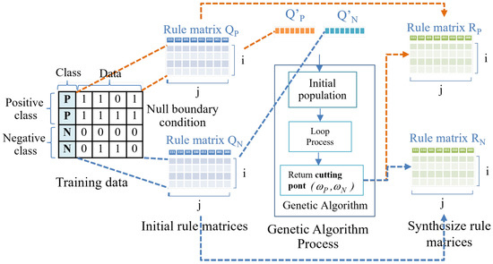
Figure 1. CAC rule ordering.

The next two states $Q_{R^{+}}^{t+1}$ and $Q_{R^{-}}^{t+1}$ are generated as follows in Equations (2) and (3)

$$Q_{R^{+}}^{t+1}=(R^{+},Q^t)$$

(2)

$$Q_{R^{-}}^{t+1}=(R^{-},Q^t)$$

(3)

As shown in Figure 1, the process of ordering the rule matrices using the initial rule matrices $\left[Q_P\right]$ and $\left[Q_N\right]$ in the first step consists of continuous data. Rule matrices with values of 0 and 1 resulting from the rule ordering process transform the data from a fuzzy set into a discrete set.

2.2. An Enhanced Butterfly Optimization Algorithm (m-MBOA)

The m-MBOA is an improved BOA with the mutualism phase of the SOS algorithm to determine the characteristics of the relationship between the two organisms.

The effectiveness of m-MBOA depends on variable configurations to control the probability that the simulated butterfly will either fly directly to the food source or fly randomly [39,40]. Its structure is mostly based on the butterfly prey approach, which employs scent recognition to detect the location of sustenance or mating sets. The discovery and handling concept is based on three critical conditions: fragrance $\left(f\right)$, sensory exposure $\left(c\right)$, stimulus intensity $\left(I\right)$, and power $\left(a\right)$. Based on these hypotheses, the fragrance in the BOA is described as a component of the boost’s physical strength, as follows:

$$f=c{I}^a$$

(4)

where f represents the magnitude of scent recognition, i.e., the intensity of smell identification by other butterflies; c represents the sensory receptor; I represents the stimulating force, and a represents the exponent power, depending on the modality. The m-MBOA has four phases: (1) startup, (2) iteration, (3) mutualism, and (4) recursive search in the initial m-MBOA operation. The algorithm is terminated at the last stage after obtaining the best response.

In the first step, the algorithm determines the problem-solving region and function purpose, as well as the parameters used in the m-MBOA set. The butterfly’s position in the search zone was generated at random, and its fragrance and suitability values were computed and stored. Further parts of this technique involve initial and recursive phase computations. An algorithm is used to accomplish the second stage of the method, which is the looping phase and several iterations. All butterflies in the solution region are transferred to a new position and evaluated for suitability in each iteration. The first algorithm determines the suitability of all butterflies in various spots in the solution region. These butterflies then use Equation (4) to produce smells based on their position. This method has two critical steps: the local and global search algorithms. Butterflies go to the most appropriate butterfly $g^{*}$ response in the global search process, as stated by Equation (5).

$$b_i^{t+1}=b_i^t+(r^2\times g^{*}-b_i^t)\times f_i$$

(5)

where $g^{*}$ is the best solution for all butterflies in the current iteration, $b_i^t$ is the ith butterfly number in iteration t, $f_i$ is the fragrance of the ith butterfly, and a random number [0, 1] is represented by r. The next best butterfly position is as follows (6).

$$b_i^{t+1}=b_i^t+(r^2\times b_j^t-b_k^t)\times f_i$$

(6)

where $b_j^t$ and $b_k^t$ are the jth and kth butterfly positions in the solution space. If $b_j^t$ and $b_k^t$ result in the same local space, and random numbers between $[0,1]$ are represented by the parameter r, then Equation (6) is the result of the random butterfly behavior. An additional phase is then used to calculate the symbolic relation of the two distinct m-MBOAs, which calculates the mutual phase in the last decision using Equations (7) and (8).

$$b_{inew}=b_i+rand[0,1]\times (b_{best}-Mutua{l}_{Vector}\times BF1)$$

(7)

$$b_{jnew}=b_j+rand[0,1]\times (b_{best}-Mutua{l}_{Vector}\times BF2)$$

(8)

where $b_{inew}$ and $b_{jnew}$ is a new butterfly value, the $Mutua{l}_{Vector}$ from (9) is used randomly. $b_{best}$ is the final solution answer; BF1 and BF2 are the random numbers of benefit factors 1 and 2, respectively.

$$Mutua{l}_{Vector}=(b_i\times b_j)/2$$

(9)

where $Mutua{l}_{Vector}$ is a mean of butterfly vector $b_i$ and $b_j$.

The threshold for stopping an answer can be defined in many ways. For example, it can be determined by the operation of the CPU, the number of calculation cycles, or the error value that occurs. If there is no error, the calculation can be stopped. This algorithm exports the most appropriate solution. The three steps described above comprise the complete algorithm of the butterfly optimization algorithms, as shown in Algorithm 1.

Algorithm 1: m-MBOA.

3. Proposed Method

We propose a novel classifier-based elementary cellular automaton that uses the variance of the initial rule matrices. In this section, several preliminaries are presented, and some essential equations are simplified. Additionally, we present the motivation for the model based on the limitations of the traditional classifier. In Table 1, we first introduce some notations that are frequently used in this study.

Table 1. Notation.

Notation	Description
$i,j$	Number of datasets (binary data) features, number of possible ECA configuration $(2^3=8)$
k	Number of samples from $U_p$ and $U_n$= 2
$U_p\in {\mathbb{R}}^{i\times j}$	Initial rule matrix of the data in positive class
$U_n\in {\mathbb{R}}^{i\times j}$	Initial rule matrix of the data in negative class
$V\in {\mathbb{R}}^{i\times j}$	Variance Decision Table matrix
$V^{{}^{\prime }}$	Variance Decision Table vector
$W_p\in {\mathbb{R}}^{i\times j}$	Rule matrix of the positive class
$W_n\in {\mathbb{R}}^{i\times j}$	Rule matrix of the negative class
$\overline{x}$	Mean of each ${\left[U_p\right]}_{ij}$ and ${\left[U_n\right]}_{ij}$
S	Standard deviation of each ${\left[U_p\right]}_{ij}$ and ${\left[U_n\right]}_{ij}$
$\%CV$	Percentage coefficient of variance
${\mathcal{D}}_t$	Training data
${\omega }_v$	The variation coefficient

First, let us provide an example of the equations for finding the rule matrices according to Equations (10) and (11) before analyzing the problem.

$${\left[R^{+}\right]}_{ij}=\left\{\begin{array}{cc}1,\hfill & {\left[U_p\right]}_{ij}\ge {\omega }_p\hfill \\ 0,\hfill & otherwise\hfill \end{array}\right.$$

(10)

$${\left[R^{-}\right]}_{ij}=\left\{\begin{array}{cc}1,\hfill & {\left[U_n\right]}_{ij}\ge {\omega }_n\hfill \\ 0,\hfill & otherwise\hfill \end{array}\right.$$

(11)

where $R^{+}$ and $R^{-}$ are the rule matrices of the positive and negative classes, respectively; ${\omega }_p$ and ${\omega }_n$ are the cutting-point decisions used to eliminate some values from the initial rule matrices $U_p$ and $U_n$ in the ith column and jth row, respectively, where $i,j=1,2,3\dots ,n$ in order to generate rule matrices with the best classification accuracy.

Definition 1 

(conflict value). A conflict value is the difference between the same position element of the initial rule matrices $\left[U_p\right]ij$ and $\left[U_n\right]ij$, arising from the creation processes of the rule matrices $\left[R^{+}\right]ij$ and $\left[R^{-}\right]ij$. The conflict value can be represented by Equation (12).

$$Conflictvalue=\left\{\begin{array}{cc}|{\left[U_p\right]}_{ij}-{\left[U_n\right]}_{ij}|,\hfill & {\left[U_p\right]}_{ij}and{\left[U_n\right]}_{ij}\ge 1\hfill \\ 0,\hfill & {\left[U_p\right]}_{ij}or{\left[U_n\right]}_{ij}=0\hfill \end{array}\right.$$

(12)

where $Conflictvalue\in I^{+}$

Lemma 1. 

The higher the conflict value the lower the classification accuracy.

Proof of Lemma 1. 

Equations (10) and (11) show that all elements of ${\left[U_p\right]}_{ij}$ and ${\left[U_n\right]}_{ij}$ would convert to 1 if their value is greater than 0.

Assume that $U_p\gg U_n$ when $\underset{x\to \infty }{lim}{\left[U_p\right]}_{ij}=\infty$ and $\underset{x\to \infty }{lim}{\left[U_n\right]}_{ij}=1$ then

$$\begin{array}{c}Conflictvalue=|{\left[U_p\right]}_{ij}-{\left[U_n\right]}_{ij}|\hfill \\ =\infty -1\hfill \\ =\infty \hfill \end{array}$$

(13)

From the above Equation (13), the conflict value $\left[U_p\right]ij$ is much greater than $\left[U_n\right]ij$. The conflict value is equivalent to the maximum value. However, from (10) and (11), it can be observed that small values are equalized with large values. Unfair behavior leads to an unreasonable increase in the amount of data. This increase in the number affects the prediction of the test data because both $\left[U_p\right]ij$ and $\left[U_n\right]ij$ are converted to 1 in the rule ordering process.    □

Definition 2 

(percentage of variation coefficient). The coefficient of variation ($CV$) is defined as the ratio of the standard deviation (S) in Equation (14) and the sample mean ($\overline{x}$) in Equation (15).

$$\overline{x}=\frac{{\displaystyle \sum _{k=1}^n}{x}_k}{N}$$

(14)

where $\overline{x}$ represents the sample mean of the elements at the same position in the initial rule matrices $\left[U_p\right]$ and $\left[U_n\right]$. $x_k$ is the observed value, where $k=(1,2,\dots ,n)$, and N represents the total number of observations. In this particular case, the number of observations is always $N=2$.

$$S=\sqrt{\sum _{k=1}^n\left(\frac{{(x_k-\overline{x})}^2}{N-1}\right)}$$

(15)

where S is the standard deviation of the elements in the initial rule matrices $U_p$ and $U_n$ at corresponding positions and the percentage $CV$ ($\%CV$) can be represented as (16)

$$\%CV=\frac{S}{\overline{x}}\times 100$$

(16)

Lemma 2. 

The percentage coefficient of variance can measure the classification ability of the initial rule matrices for each position.

To make all positions of the initial matrix comparable, we used the percentage coefficient of variation to measure the abilities of each initial rule matrix position, instead of using direct conflict values that do not allow for comparisons.

Proof of Lemma 2. 

First, we simplify (16) to calculate the $\%CV$ of matrices $U_p$ and $U_n$ as follows:

Represent $\overline{x}$($U_p$, $U_n$) for each element, i is the row and j is the column of matrices $U_p$ and $U_n$ as following (17)

$$\begin{array}{c}\overline{x}(U_p,U_n)={\displaystyle \frac{{\left[U_p\right]}_{ij}+{\left[U_n\right]}_{ij}}{2}}\hfill \end{array}$$

(17)

Substituting $N=2$, x = ${\left[U_p\right]}_{ij}$ and ${\left[U_n\right]}_{ij}$ into (15)

$$\begin{array}{c}S(U_p,U_n)=\sqrt{{\displaystyle \frac{{({\left[U_p\right]}_{ij}-\overline{x})}^2+{({\left[U_n\right]}_{ij}-\overline{x})}^2}{2-1}}}\hfill \\ \\ =\sqrt{{({\left[U_p\right]}_{ij}-\overline{x})}^2+{({\left[U_n\right]}_{ij}-\overline{x})}^2}\hfill \end{array}$$

(18)

Substitute $\overline{x}(U_p$, $U_n)$ from (17) in (18), we obtain:

$$\begin{array}{c}S=\sqrt{{\left({\left[U_p\right]}_{ij}-\left({\displaystyle \frac{{\left[U_p\right]}_{ij}+{\left[U_n\right]}_{ij}}{2}}\right)\right)}^2+{\left({\left[U_n\right]}_{ij}-\left({\displaystyle \frac{{\left[U_p\right]}_{ij}+{\left[U_n\right]}_{ij}}{2}}\right)\right)}^2}\hfill \\ \\ =\sqrt{{\left({\displaystyle \frac{2{\left[U_p\right]}_{ij}-{\left[U_p\right]}_{ij}-{\left[U_n\right]}_{ij}}{2}}\right)}^2+{\left({\displaystyle \frac{2{\left[U_n\right]}_{ij}-{\left[U_p\right]}_{ij}-{\left[U_n\right]}_{ij}}{2}}\right)}^2}\hfill \\ \\ =\sqrt{{\left({\displaystyle \frac{{\left[U_p\right]}_{ij}-{\left[U_n\right]}_{ij}}{2}}\right)}^2+{\left({\displaystyle \frac{{\left[U_n\right]}_{ij}-{\left[U_p\right]}_{ij}}{2}}\right)}^2}\hfill \\ \\ =\sqrt{{\displaystyle \frac{{({\left[U_p\right]}_{ij}-{\left[U_n\right]}_{ij})}^2+{({\left[U_n\right]}_{ij}-{\left[U_p\right]}_{ij})}^2}{4}}}\hfill \end{array}$$

(19)

Assuming that

$${\displaystyle \frac{{({\left[U_p\right]}_{ij}-{\left[U_n\right]}_{ij})}^2}{4}}={\displaystyle \frac{{({\left[U_n\right]}_{ij}-{\left[U_p\right]}_{ij})}^2}{4}}$$

(20)

where ${\displaystyle \frac{{({\left[U_p\right]}_{ij}^{{}^{\prime }}-{\left[U_n\right]}_{ij}^{{}^{\prime }})}^2}{4}},{\displaystyle \frac{{({\left[U_n\right]}_{ij}-{\left[U_p\right]}_{ij})}^2}{4}}\in {\mathbb{R}}^{+}$.

Substitute Equation (20) in to Equation (19)

$$\begin{array}{cc}\hfill S& =\sqrt{\frac{{({\left[U_p\right]}_{ij}-{\left[U_n\right]}_{ij})}^2}{4}+\frac{{({\left[U_p\right]}_{ij}-{\left[U_n\right]}_{ij})}^2}{4}}\hfill \\ & =\sqrt{2\frac{{({\left[U_p\right]}_{ij}-{\left[U_n\right]}_{ij})}^2}{4}}\hfill \\ & =\frac{\left|{\left[U_p\right]}_{ij}-{\left[U_n\right]}_{ij}\right|}{\sqrt{2}}\hfill \end{array}$$

(21)

Substituting $\overline{x}$ and S from (17) and (21) into (16)

$$\begin{array}{cc}\hfill \%C{V}_{ij}& ={\displaystyle \frac{{\displaystyle \frac{\left|{\left[U_p\right]}_{ij}-{\left[U_n\right]}_{ij}\right|}{\sqrt{2}}}}{{\displaystyle \frac{{\left[U_p\right]}_{ij}+{\left[U_n\right]}_{ij}}{2}}}}\times 100\hfill \\ & =\left\{\begin{array}{c}\sqrt{2}{\displaystyle \frac{\left|{\left[U_p\right]}_{ij}-{\left[U_n\right]}_{ij}\right|}{{\left[U_p\right]}_{ij}+{\left[U_n\right]}_{ij}}}\times 100,{\left[U_p\right]}_{ij}+{\left[U_n\right]}_{ij}>0\hfill \\ 0,otherwise\hfill \end{array}\right.\hfill \end{array}$$

(22)

Assuming that ${\left[U_p\right]}_{ij}>{\left[U_n\right]}_{ij}$ then

$$\begin{array}{c}Conflictvalue=|{\left[U_p\right]}_{ij}-{\left[U_n\right]}_{ij}|\hfill \end{array}$$

(23)

Substitute (23) into (22), then

$$\begin{array}{c}\%C{V}_{ij}=\left\{\begin{array}{c}\sqrt{2}{\displaystyle \frac{\left(Conflictvalue\right)}{{\left[U_p\right]}_{ij}+{\left[U_n\right]}_{ij}}}\times 100,{\left[U_p\right]}_{ij}+{\left[U_n\right]}_{ij}>0\hfill \\ 0,otherwise\hfill \end{array}\right.\hfill \end{array}$$

(24)

From Equation (24), we can observe that as the conflict value increases, the percentage of variance also increases. This implies that the two values are directly proportional to each other, indicating that the percentage variance can be used to measure classification ability.    □

Lemma 3. 

Eliminating the element with the lower value could improve classification accuracy.

Proof of Lemma 3. 

Assuming that ${\left[U_p\right]}_{ij}\gg {\left[U_n\right]}_{ij}$ and ${\omega }_p,{\omega }_n$ = 0 from (10) and (11), then

$$\begin{array}{c}Conflictvalue={\left[U_p\right]}_{ij}-{\left[U_n\right]}_{ij}\hfill \\ \\ Conflictvalue\approx {\left[U_p\right]}_{ij}\hfill \end{array}$$

(25)

where ${\left[U_n\right]}_{ij}$ > 0.

From Equation (25), if we set $\left[U_n\right]ij$ to 0, only the data for $\left[U_n\right]ij$ will be lost, where $\underset{x\to \infty }{lim}\left[U_n\right]ij=1$. From (24), we can reduce the $conflictvalue$ and $\%CV$ by setting $\left[U_p\right]ij$ to 0. This means that the classifier can better classify patterns because a lower $\%CV$ indicates greater classification ability.    □

Definition 3 

(Variance decision table). The variance decision table (V) is the $\%CV$ representation in the matrix form.

Definition 4 

(Loss of data). The loss of data is part of the data converted to zero to improve overall classification accuracy.

Lemma 4. 

Appropriate estimation of the percentage coefficient of variance can produce a suitable rule matrix.

Proof of Lemma 4. 

From Lemma 3 $min({\left[U_p\right]}_{ij},{\left[U_n\right]}_{ij})$ is eliminated to increase the ability to classify patterns when ${\left[U_p\right]}_{ij}\gg {\left[U_n\right]}_{ij}$ or ${\left[U_n\right]}_{ij}\gg {\left[U_p\right]}_{ij}$.

However, when ${\left[U_p\right]}_{ij}\approx {\left[U_n\right]}_{ij}$, if we convert $min({\left[U_p\right]}_{ij},{\left[U_n\right]}_{ij})$ to 0, loss of data $\approx {\left[U_p\right]}_{ij}$ and ${\left[U_n\right]}_{ij}$, which could result in overfitting of the classifier model. Appropriate approximations were used to prevent the above problems and to obtain results that provided the best classification capability.    □

Definition 5 

(Variation coefficient). The variation coefficient (${\omega }_v$) was obtained using V. This was estimated using the m-MBOA algorithm, which can be used to generate the best rule matrices in the synthesis process.

Theorem 1. 

The coefficient of variation and variance decision table can create effective rule matrices for the classification.

3.1. Proposed Method

This paper proposes an efficient cellular automata-based classifier with a variance decision table (CAV). We present this algorithm in Algorithm 2. As a result, when using only the estimated random border to determine the class using the GA in rule ordering, the traditional technique has a classification accuracy problem and cannot handle high-dimensional problems. This work overcomes this limitation by adopting a unique butterfly optimization technique (m-MBOA) instead of the genetic approach depicted in Figure 2.

Algorithm 2: CAV labeled.

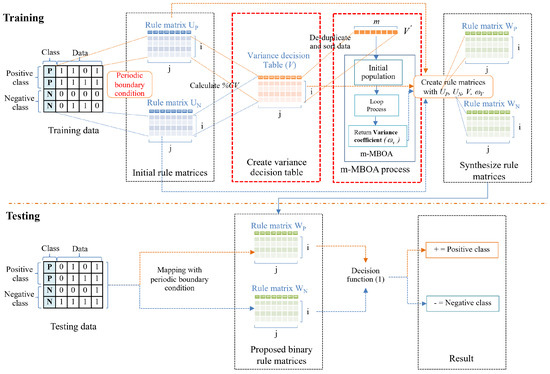
Figure 2. An overview of the proposed CAV methods.

3.1.1. Initial Values of Rule Matrices

If the input data is not binary, the rule ordering procedure begins by converting it to binary code using a Gray code [41,42,43] encoder. Cyclical or periodic [44,45] boundary conditions are used to maximize the rule-output equality of the available systems, whereas null boundary conditions can be relied upon to increase the overall complexity of a system [46,47]. Figure 3 shows $U_p$ and $U_n$ are the initial rule matrices created by counting the $PAB$ and $NAB$ attractor basins, respectively. The initial rule matrix $U_p$ is represented in matrix form with the ith $(i=1,2,\dots ,n)$ row and the jth $(j=1,2,\dots ,n)$ column. The rows reflect the number of binary features in the data, and the columns represent the number of patterns from $PAB$ in which the nearest neighbors $(U_{i-1}^t,U_i^t,U_{i+1}^t)$ for the $ith$ cell decoded to decimal must equal j. Similarly, $NAB$ is used to formulate an element of matrix $U_n$.

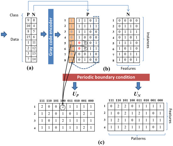
Figure 3. The initial rule matrices process consists of three steps: (a) converting the input data into binary data using a gray code encoder; (b) creating initial rule matrices with periodic boundary conditions; and (c) generating initial rule matrices for both positive and negative data.

3.1.2. Create Variance Decision Table

The variance decision table (V) corrects the percentage of the variance coefficient value and is represented in matrix form.

Subsequently, (22) is used to generate the variance decision table when ${\left[U_p\right]}_{ij}+{\left[U_n\right]}_{ij}>0.$

$$V=\left[\begin{array}{cccc}\%C{V}_{11}& \%C{V}_{12}& ···& \%C{V}_{18}\\ \%C{V}_{21}& \%C{V}_{22}& \cdots & \%C{V}_{28}\\ ⋮& ⋮& \ddots & ⋮\\ \%C{V}_{n1}& \%C{V}_{n2}& ···& \%C{V}_{n8}\end{array}\right]$$

(26)

where n refers to the number of features in the dataset represented by the binary patterns. An example of creating a variance decision table is shown in Figure 4.

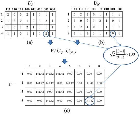
Figure 4. The Create Variance Decision Table process. (a) Initial rule matrix of positive data; (b) initial rule matrix of negative data; and (c) generating variance decision table.

3.1.3. m-MBOA Process

The CAV starts by transforming V into vector $V^{\prime }$ under the following conditions, as shown in Figure 5:

Figure 5. The m-MBOA process. (a) Variance decision table; (b) Create vector V′ by de-duplicate and sort data; (c) process m-MBOA algorithm to create the variation coefficient; and (d) variation coefficient.

Matrix V is transformed into an array that is sorted but not complete, and the result is stored in array $V^{\prime }$. The result from m-MBOA includes a variable, the variation coefficient (${\omega }_v$), which serves as a threshold that helps the classifier converge to the best solution for creating rule matrices using Equations (27) and (28).

3.1.4. Rule Matrices Synthesis

Under the following conditions, this is the final stage in generating the rule matrices.

$${\left[W_p\right]}_{ij}=\left\{\begin{array}{cc}1,\hfill & {\left[U_p\right]}_{ij}\ge {\left[U_n\right]}_{ij}or{V}_{ij}\le {\omega }_v\hfill \\ 0,\hfill & otherwise\hfill \end{array}\right.$$

(27)

$${\left[W_n\right]}_{ij}=\left\{\begin{array}{cc}1,\hfill & {\left[U_n\right]}_{ij}\ge {\left[U_p\right]}_{ij}or{V}_{ij}\le {\omega }_v\hfill \\ 0,\hfill & otherwise\hfill \end{array}\right.$$

(28)

where ${\omega }_v$ is the threshold required to converge the model to the best answer.

Although the CAV uses the same process as the traditional classifier for synthesizing the rule matrices, each element is compared between the positive and negative values of the initial rule matrices and ${\omega }_v$. The CAV improves the performance of generating the final rule matrices by using the statistical relationship between $U_p$ and $U_n$. We can obtain a better quality rule matrix than with the traditional method, as shown in the example in Figure 6.

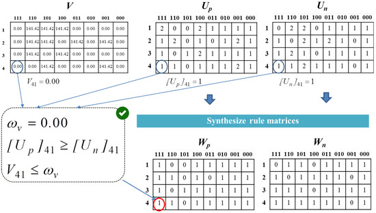
Figure 6. Synthesis rule matrices.

4. Experimentals

In this part, we present a method for assessing the effectiveness of the suggested classifier. The datasets, classifier comparison, and commentary are all given.

4.1. Experimental Setup

The classification accuracy of the classifiers was tested with both training and sample data, using 10-fold cross-validation as per CAV. A confusion matrix was utilized to determine the accuracy of classification. For multiclass classification, CAV implements a DDAG scheme [48]. To evaluate the performance of the model, standard classifiers were utilized, and non-binary datasets were first converted into Gray code during the preprocessing phase.

We compared the accuracy, precision, recall, F1, specificity, and G-mean between CAV, CAC, and several well-known classifiers, including SVM, kNN, Naïve Bayes, and two dense neural networks methods, DNN-1 and DNN-2. The DNN-1 and DNN-2 methods were distinguished by different activation functions, hidden layer numbers, and hidden layer sizes.

Finally, the butterfly optimization parameters were set up in the last preprocessing step, using the configuration shown in Table 2, to achieve optimal performance for the proposed method.

Table 2. Classification method parameters.

Classifier	Parameters	Value
CAV	Population	100
	Probability switch (p)	0.5
	Power exponent	0.4
	Sensory modality	0.03
	Max iteration	20
CAC	Sample	100
	Crossover probability	48
	Mutation probability	40
	Max iteration	20
SVM	SVM type	C-SVM
	Kernel type	Rbf
	Class weight	1.0
kNN	K (neighbor)	5
	Weighted vote	Yes
DNN-1	Activation	Rectifier
	Hidden layer number	2
	Hidden layer size	50
DNN-2	Activation	Maxout
	Hidden layer number	3
	Hidden layer size	100
Naïve Bayes	Laplace correction	Yes

4.2. Datasets

Datasets from the OpenML repository were used, consisting of different types of instances, features, and numbers of dataset classes, as shown in Table 3. The results demonstrate that the datasets form clusters, as shown by Analcatdata boxing2 (Figure 7a), Breast_w dataset (Figure 7b), Prnn synth (Figure 7d), and Mammographic mass dataset (Figure 7h), which clustered with the mean datasets. However, non-conforming data, such as Hayes roth (Figure 7c), Tae (Figure 7e), Wisconsin (Figure 7f), and SPECTheart (Figure 7g), were identified. The scatter plot results reveal ambiguous data, as most of the data from different classes are mixed, and the classification accuracy is lower when dealing with this type of data.

Table 3. Datasets.

Dataset	Class	Instances	Features
Soybean (small)	4	47	35
SPECT heart	2	80	23
Analcatdata boxing2	2	132	10
Tae	3	151	6
Hayes-Roth	3	160	5
Wisconsin	2	194	33
Sonar	2	208	61
Prnn synth	2	256	3
Thyroid Disease	2	306	3
Ecoli	8	336	8
Congressional Voting	2	435	16
Monk Problem 2	2	601	7
Breast w	2	699	10
Pima Indians Diabetes	2	768	8
Mammographic Mass	2	961	6

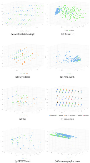
Figure 7. Illustration of dataset distribution using the PCA technique.

4.3. Classifier Performance Evaluation Method

This step involves a testing process to validate the algorithm’s classification capability and compare the performance of each model. We have chosen the following parameters: accuracy, precision, recall, F1, specificity, and G-mean. Accuracy (29) measures the model’s performance as the ratio of correctly computed data to all the data. Precision (30) is the proportion of positive data accurately measured. Recall (31) is a parameter that indicates the efficiency of positive data classification. F1 (32) is the harmonic mean of accuracy and recall, which provides an idea of the accuracy and efficiency of positive data classification. Next, the Specificity (33) parameter calculates the true proportion of validity measures for negative data, where the performance of both positive and negative data can be derived and determined using G-mean (34).

$$\begin{array}{c}Accuracy={\displaystyle \frac{a+b}{a+b+c+d}}\times 100\hfill \end{array}$$

(29)

$$\begin{array}{c}Precision={\displaystyle \frac{a}{a+c}}\hfill \end{array}$$

(30)

$$\begin{array}{c}Recall={\displaystyle \frac{a}{a+d}}\hfill \end{array}$$

(31)

$$\begin{array}{c}F1={\displaystyle \frac{2(Precision\times Recall)}{(Precision+Recall)}}\hfill \end{array}$$

(32)

$$\begin{array}{c}Specificity={\displaystyle \frac{b}{b+d}}\hfill \end{array}$$

(33)

$$\begin{array}{c}G-mean=\sqrt{Recall\times Specificity}\hfill \end{array}$$

(34)

where a is a true positive ($T{P}_i$), b is a true negative ($T{N}_i$), c is false positive ($F{P}_i$), and d is false negative ($F{N}_i$), all define parameters based on confusion matrix structure.

5. Results and Discussion

Experiments were conducted on 15 OpenML datasets with varying instances and feature numbers to evaluate performance in terms of accuracy, precision, recall, F1, specificity, and G-mean, which are shown in Table 4, Table 5, Table 6, Table 7, Table 8 and Table 9, with the best performance highlighted. A comparison of the classification results between CAV and the other classifiers is also summarized in Figure 8, Figure 9, Figure 10, Figure 11, Figure 12 and Figure 13.

Table 4. The accuracy of the proposed CAV compared with CAC, SVM, k-NN, DNN-1, DNN-2, and naïve Bayes (the bold number indicates the maximum value).

Dataset	Classification Accuracy (K = 10)							Average Improvement
	CAV	CAC	SVM	kNN	DNN-1	DNN-2	Naïve Bayes
Analcatdata boxing2	72.360	69.200	71.970	64.390	56.820	63.640	67.420
Breast w	97.420	96.850	96.850	97.000	96.570	96.570	95.990
Congressional voting	96.980	95.270	92.240	93.970	95.260	95.260	94.830
Ecoli	88.240	67.510	43.740	85.120	81.850	79.510	79.170
Hayes-Roth	78.950	77.250	43.750	66.250	58.750	66.870	70.000
Mammographic mass	82.640	82.430	80.480	79.520	82.170	81.330	80.600
Monk’s problems 2	67.500	63.400	82.530	66.560	63.890	74.210	64.390
Pima indian diabetes	72.700	69.263	72.010	71.740	74.220	74.350	75.520
Prnn synth	83.279	78.704	84.400	81.600	83.200	82.800	84.400
Sonar	74.550	74.143	87.020	80.290	80.290	81.250	67.790
Soybean small	100.000	100.000	100.000	97.870	100.000	100.000	100.000
SPECTheart	75.000	62.500	68.750	63.750	71.250	71.250	68.750
Tae	59.040	57.536	47.020	47.680	46.360	41.720	51.660
Thyroid disease	93.960	94.892	80.930	95.350	93.490	93.490	96.740
Wisconsin	97.510	97.217	97.070	97.360	96.930	96.930	96.190
Average	82.675	79.078	76.584	79.230	78.737	79.945	79.563
Improvement		3.60	6.09	3.45	3.94	2.73	3.11	4.58

Table 5. The precision of the proposed CAV compared with CAC, SVM, k-NN, DNN-1, DNN-2 and naïve Bayes (the bold number indicates the maximum value).

Dataset	Classification Accuracy (K = 10)							Average Improvement
	CAV	CAC	SVM	kNN	DNN-1	DNN-2	Naïve Bayes
Analcatdata boxing2	0.720	0.750	0.873	0.747	0.521	0.648	0.761
Breast w	0.993	0.994	0.972	0.974	0.965	0.965	0.952
Congressional voting	0.983	0.977	0.887	0.927	0.944	0.960	0.960
Ecoli	0.880	0.723	0.088	0.558	0.595	0.739	0.547
Hayes-Roth	0.835	0.830	0.366	0.637	0.631	0.693	0.751
Mammographic mass	0.815	0.803	0.873	0.814	0.772	0.757	0.811
Monk’s problems 2	0.889	0.727	0.779	1.000	0.527	0.676	0.980
Pima indian diabetes	0.809	0.846	0.466	0.519	0.474	0.489	0.605
Prnn synth	0.854	0.789	0.832	0.920	0.776	0.760	0.848
Sonar	0.744	0.786	0.814	0.722	0.773	0.835	0.804
Soybean small	1.000	1.000	1.000	0.975	1.000	1.000	1.000
SPECTheart	0.815	0.583	0.450	0.450	0.700	0.700	0.450
Tae	0.629	0.622	0.468	0.475	0.461	0.410	0.518
Thyroid disease	0.927	0.940	0.580	0.910	0.863	0.911	0.965
Wisconsin	0.991	0.991	0.973	0.978	0.964	0.964	0.955
Average	0.859	0.824	0.695	0.774	0.731	0.767	0.794
Improvement		0.035	0.164	0.085	0.128	0.092	0.065	0.114

Table 6. The recall of the proposed CAV compared with CAC, SVM, k-NN, DNN-1, DNN-2 and naïve Bayes (the bold number indicates the maximum value).

Dataset	Classification Accuracy (K = 10)							Average Improvement
	CAV	CAC	SVM	kNN	DNN-1	DNN-2	Naïve Bayes
Analcatdata boxing2	0.631	0.500	0.689	0.646	0.617	0.667	0.675
Breast w	0.967	0.958	0.980	0.980	0.982	0.982	0.986
Congressional voting	0.960	0.935	0.965	0.958	0.967	0.952	0.944
Ecoli	0.835	0.700	0.200	0.551	0.571	0.755	0.563
Hayes-Roth	0.798	0.783	0.601	0.735	0.615	0.679	0.742
Mammographic mass	0.834	0.851	0.760	0.775	0.847	0.843	0.794
Monk’s problems 2	0.400	0.400	0.849	0.663	0.874	0.908	0.653
Pima indian diabetes	0.760	0.646	0.635	0.612	0.690	0.686	0.664
Prnn synth	0.791	0.808	0.853	0.762	0.874	0.880	0.841
Sonar	0.819	0.728	0.898	0.833	0.798	0.779	0.619
Soybean small	1.000	1.000	1.000	0.986	1.000	1.000	1.000
SPECTheart	0.700	0.500	0.857	0.628	0.718	0.718	0.857
Tae	0.589	0.576	0.469	0.479	0.511	0.282	0.513
Thyroid disease	0.927	0.925	0.806	0.960	0.962	0.911	0.942
Wisconsin	0.971	0.966	0.982	0.982	0.989	0.989	0.986
Average	0.799	0.752	0.769	0.770	0.801	0.802	0.785
Improvement		0.047	0.029	0.029	−0.002	−0.003	0.014	0.023

Table 7. The F1 of the proposed CAV compared with CAC, SVM, k-NN, DNN-1, DNN-2 and naïve Bayes (the bold number indicates the maximum value).

Dataset	Classification Accuracy (K = 10)							Average Improvement
	CAV	CAC	SVM	kNN	DNN-1	DNN-2	Naïve Bayes
Analcatdata boxing2	0.662	0.600	0.770	0.693	0.565	0.657	0.715
Breast w	0.980	0.975	0.976	0.977	0.974	0.974	0.969
Congressional voting	0.971	0.971	0.924	0.943	0.955	0.956	0.953
Ecoli	0.850	0.921	0.122	0.553	0.574	0.738	0.544
Hayes-Roth	0.786	0.788	0.310	0.663	0.622	0.685	0.742
Mammographic mass	0.823	0.825	0.813	0.794	0.808	0.797	0.803
Monk’s problems 2	0.552	0.516	0.812	0.797	0.657	0.775	0.783
Pima indian diabetes	0.784	0.732	0.538	0.562	0.562	0.571	0.633
Prnn synth	0.817	0.789	0.842	0.833	0.822	0.816	0.845
Sonar	0.773	0.748	0.854	0.774	0.785	0.806	0.700
Soybean small	1.000	1.000	1.000	0.980	1.000	1.000	1.000
SPECTheart	0.730	0.529	0.590	0.651	0.709	0.709	0.590
Tae	0.569	0.551	0.464	0.474	0.445	0.327	0.501
Thyroid disease	0.914	0.927	0.600	0.932	0.971	0.911	0.953
Wisconsin	0.980	0.978	0.977	0.980	0.976	0.976	0.970
Average	0.813	0.790	0.706	0.774	0.762	0.780	0.780
Improvement		0.023	0.107	0.039	0.051	0.033	0.033	0.057

Table 8. The specificity of the proposed CAV compared with CAC, SVM, k-NN, DNN-1, DNN-2 and naïve Bayes (the bold number indicates the maximum value).

Dataset	Classification Accuracy (K = 10)							Average Improvement
	CAV	CAC	SVM	kNN	DNN-1	DNN-2	Naïve Bayes
Analcatdata boxing2	0.804	0.857	0.786	0.640	0.528	0.603	0.673
Breast w	0.988	0.988	0.947	0.951	0.936	0.936	0.914
Congressional voting	0.981	0.973	0.881	0.920	0.937	0.953	0.953
Ecoli	0.850	0.921	0.000	0.978	0.973	0.948	0.969
Hayes-Roth	0.887	0.873	0.718	0.819	0.777	0.823	0.837
Mammographic mass	0.820	0.799	0.861	0.816	0.801	0.791	0.818
Monk’s problems 2	0.675	0.857	0.807	1.000	0.485	0.583	0.000
Pima indian diabetes	0.727	0.780	0.750	0.762	0.759	0.763	0.798
Prnn synth	0.872	0.767	0.836	0.899	0.799	0.789	0.847
Sonar	0.663	0.753	0.850	0.782	0.807	0.846	0.768
Soybean small	1.000	1.000	1.000	0.993	1.000	1.000	1.000
SPECTheart	0.800	0.750	0.627	0.649	0.707	0.707	0.627
Tae	0.795	0.789	0.737	0.739	0.735	0.724	0.768
Thyroid disease	0.960	0.960	0.809	0.975	0.935	0.951	0.971
Wisconsin	0.983	0.983	0.951	0.959	0.936	0.936	0.921
Average	0.854	0.870	0.771	0.859	0.808	0.824	0.791
Improvement		−0.016	0.083	−0.005	0.046	0.030	0.063	0.040

Table 9. The G-mean of the proposed CAV compared with CAC, SVM, k-NN, DNN-1, DNN-2, and naïve Bayes (the bold number indicates the maximum value).

Dataset	Classification Accuracy (K = 10)							Average Improvement
	CAV	CAC	SVM	kNN	DNN-1	DNN-2	Naïve Bayes
Analcatdata boxing2	0.712	0.655	0.736	0.643	0.571	0.634	0.674
Breast w	0.977	0.973	0.963	0.965	0.959	0.959	0.950
Congressional voting	0.970	0.954	0.922	0.939	0.952	0.953	0.949
Ecoli	0.843	0.803	0.000	0.734	0.745	0.846	0.738
Hayes-Roth	0.841	0.827	0.657	0.776	0.691	0.748	0.788
Mammographic mass	0.827	0.825	0.809	0.795	0.824	0.816	0.806
Monk’s problems 2	0.520	0.585	0.827	0.814	0.651	0.728	0.000
Pima indian diabetes	0.743	0.710	0.690	0.683	0.724	0.723	0.728
Prnn synth	0.831	0.787	0.844	0.827	0.835	0.833	0.844
Sonar	0.737	0.740	0.874	0.807	0.802	0.812	0.690
Soybean small	1.000	1.000	1.000	0.990	1.000	1.000	1.000
SPECTheart	0.748	0.612	0.733	0.638	0.713	0.713	0.733
Tae	0.684	0.674	0.587	0.595	0.612	0.452	0.628
Thyroid disease	0.943	0.942	0.808	0.967	0.948	0.931	0.956
Wisconsin	0.977	0.974	0.966	0.970	0.962	0.962	0.953
Average	0.824	0.804	0.761	0.810	0.799	0.807	0.762
Improvement		0.020	0.063	0.014	0.024	0.016	0.061	0.040

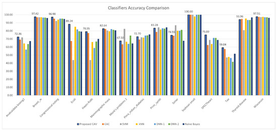
Figure 8. CAV with other classifiers; accuracy comparison for the test datasets.

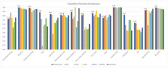
Figure 9. CAV with other classifiers; precision comparison for the test datasets.

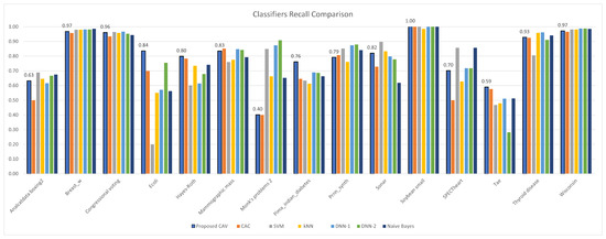
Figure 10. CAV with other classifiers; recall comparison for the test datasets.

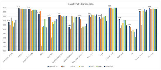
Figure 11. CAV with other classifiers; F1 comparison for the test datasets.

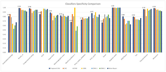
Figure 12. CAV with other classifiers; specificity comparison for the test datasets.

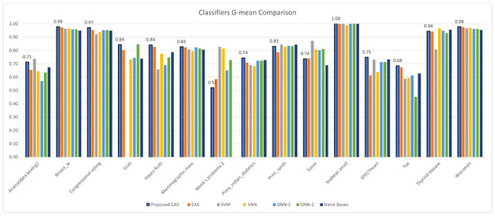
Figure 13. CAV with other classifiers; G-mean comparison for the test datasets.

In terms of classification accuracy, Table 4 shows that the proposed methods have the highest classification accuracy for the following datasets: congressional voting, monk problem 2, SPECT heart, mammographic mass, Hayes–Roth, Tae, Breast w, Analcatdata boxing2, soybean (small), and Pima Indians diabetes. For the Sonar dataset, SVM achieved the highest accuracy, while the naive Bayes algorithm was the most accurate for the thyroid disease dataset. CAV was the second-best classification result for the thyroid disease dataset, and k-NN was the best for the Ecoli dataset. SVM and naive Bayes yielded the best classification results for the Prnn synth dataset. For the Wisconsin dataset, the k-NN classifier produced the best results. The results demonstrate that CAV is the best classifier for most of the test datasets, but there are a few datasets in which it is inferior to other classification algorithms.

The average accuracy and improvement shows that the proposed algorithm can handle classification problems more efficiently than other classifiers. However, different classification models perform well only for specific datasets. Figure 14a presents an analysis of the mean classification ability, indicating that the proposed model is the most effective classifier compared to the others.

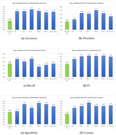
Figure 14. Illustration of the average Friedman rank for CAV, CAC, SVM, kNN, DNN-1, DNN-2, and Naïve Bayes. The green bar graph represents the value of the average Friedman rank in the proposed model, while the blue bar graph represents the corresponding value of the classifier used for comparison with the proposed model.

Conversely, the proposed method also reported high classification accuracy, which was significantly different. The classification accuracy for datasets with non-conforming patterns was much lower than that for conforming datasets due to ambiguous datasets. Nevertheless, if we consider only the correctness of the classification between CAC and CAV when comparing the classification accuracy results with the conforming pattern datasets, both obtained a high classification performance. However, CAV still obtains good results for non-conforming pattern datasets that contain more noise. In contrast, for datasets with non-conforming patterns, the classification accuracy was much lower because the dataset patterns were unclear.

In terms of classification precision (Table 5), F1 score (Table 7), and G-mean (Table 9), it can be observed that the proposed method outperforms other classifiers. Upon ranking the performance of the classifiers presented in Figure 14b,d,f, it is evident that the proposed model accurately predicted positive data, as evidenced by its high precision value. Furthermore, the proposed classifier demonstrated superior performance in handling positive data, as indicated by its high F1 score. Notably, the proposed model’s classification efficiency for both positive and negative data, as measured by the G-mean parameter, surpassed that of all other classifiers tested in the experiment. Regrettably, the proposed classifier model demonstrated suboptimal performance with respect to recall, as indicated by the values presented in Table 6, and specificity, as evidenced by the data in Table 8. Specifically, the mean of the recall sequence plotted in Figure 14c suggests that the proposed model, which incorporates correlations derived from both positive and negative data, achieved inferior results compared to DNN-1, DNN-2, and Naive Bayes. Nevertheless, the proposed model exhibited superior performance in terms of specificity, as demonstrated by its ranking relative to comparable models in Figure 14e.

6. Conclusions

The CAV is a high-performance classifier capable of handling both conforming and non-conforming binary patterns to address and solve the limitation of finding decision boundaries to divide difficult data, and GA in the rule ordering process cannot handle complicated high-dimensional problems. When tested on 15 OpenML datasets with varying examples, features, and class numbers, CAV outperformed promising state-of-the-art classification approaches such as SVM, k-NN, DNN-1, DNN-2, naive Bayes, and CAC.

To increase accuracy, the following difficulties should be addressed in future studies. First, an efficient method for transforming data into binary data, other than Gray code, must be determined. Second, multiclass classification in binary classifiers (CAC and CAV) utilizing the DDAG approach was restricted. To increase classification performance, an effective strategy may be used. Finally, in terms of classifier-based elementary cellular automata, we assume that the dataset contains equal instances for each class and does not focus on the imbalance problem. Improving the classifier performance on imbalanced data without an exciting data imbalance management method while changing the classifier process directly is an interesting area of study.

References

- Chauhan, V.K.; Dahiya, K.; Sharma, A. Problem formulations and solvers in linear SVM: A review. Artif. Intell. Rev. 2019, 52, 803–855. [Google Scholar] [CrossRef]
- Wang, S.; Tao, D.; Yang, J. Relative Attribute SVM+ Learning for Age Estimation. IEEE Trans. Cybern. 2016, 46, 827–839. [Google Scholar] [CrossRef] [PubMed]
- Ameh Joseph, A.; Abdullahi, M.; Junaidu, S.B.; Hassan Ibrahim, H.; Chiroma, H. Improved multi-classification of breast cancer histopathological images using handcrafted features and deep neural network (dense layer). Intell. Syst. Appl. 2022, 14, 200066. [Google Scholar] [CrossRef]
- Hirsch, L.; Katz, G. Multi-objective pruning of dense neural networks using deep reinforcement learning. Inf. Sci. 2022, 610, 381–400. [Google Scholar] [CrossRef]
- Lee, K.B.; Shin, H.S. An Application of a Deep Learning Algorithm for Automatic Detection of Unexpected Accidents Under Bad CCTV Monitoring Conditions in Tunnels. In Proceedings of the 2019 International Conference on Deep Learning and Machine Learning in Emerging Applications (Deep-ML), Istanbul, Turkey, 26–28 August 2019; pp. 7–11. [Google Scholar] [CrossRef]
- Roy, S.; Menapace, W.; Oei, S.; Luijten, B.; Fini, E.; Saltori, C.; Huijben, I.; Chennakeshava, N.; Mento, F.; Sentelli, A.; et al. Deep Learning for Classification and Localization of COVID-19 Markers in Point-of-Care Lung Ultrasound. IEEE Trans. Med Imaging 2020, 39, 2676–2687. [Google Scholar] [CrossRef]
- Bai, X.; Wang, X.; Liu, X.; Liu, Q.; Song, J.; Sebe, N.; Kim, B. Explainable deep learning for efficient and robust pattern recognition: A survey of recent developments. Pattern Recognit. 2021, 120, 108102. [Google Scholar] [CrossRef]
- Jang, S.; Jang, Y.E.; Kim, Y.J.; Yu, H. Input initialization for inversion of neural networks using k-nearest neighbor approach. Inf. Sci. 2020, 519, 229–242. [Google Scholar]
- González, S.; García, S.; Li, S.T.; John, R.; Herrera, F. Fuzzy k-nearest neighbors with monotonicity constraints: Moving towards the robustness of monotonic noise. Neurocomputing 2021, 439, 106–121. [Google Scholar] [CrossRef]
- Tran, T.M.; Le, X.M.T.; Nguyen, H.T.; Huynh, V.N. A novel non-parametric method for time series classification based on k-Nearest Neighbors and Dynamic Time Warping Barycenter Averaging. Eng. Appl. Artif. Intell. 2019, 78, 173–185. [Google Scholar] [CrossRef]
- Sun, N.; Sun, B.; Lin, J.D.; Wu, M.Y.C. Lossless Pruned Naive Bayes for Big Data Classifications. Big Data Res. 2018, 14, 27–36. [Google Scholar] [CrossRef]
- Zhen, R.; Jin, Y.; Hu, Q.; Shao, Z.; Nikitakos, N. Maritime Anomaly Detection within Coastal Waters Based on Vessel Trajectory Clustering and Naïve Bayes Classifier. J. Navig. 2017, 70, 648–670. [Google Scholar] [CrossRef]
- Ruan, S.; Chen, B.; Song, K.; Li, H. Weighted naïve Bayes text classification algorithm based on improved distance correlation coefficient. Neural Comput. Appl. 2021, 34, 2729–2738. [Google Scholar] [CrossRef]
- Tufail, A.B.; Anwar, N.; Othman, M.T.B.; Ullah, I.; Khan, R.A.; Ma, Y.K.; Adhikari, D.; Rehman, A.U.; Shafiq, M.; Hamam, H. Early-Stage Alzheimers Disease Categorization Using PET Neuroimaging Modality and Convolutional Neural Networks in the 2D and 3D Domains. Sensors 2022, 22, 4609. [Google Scholar] [CrossRef] [PubMed]
- Tufail, A.B.; Ma, Y.K.; Zhang, Q.N. Binary Classification of Alzheimer’s Disease Using sMRI Imaging Modality and Deep Learning. J. Digit. Imaging 2020, 33, 1073–1090. [Google Scholar] [CrossRef]
- Tufail, A.B.; Ullah, I.; Rehman, A.U.; Khan, R.A.; Khan, M.A.; Ma, Y.K.; Hussain Khokhar, N.; Sadiq, M.T.; Khan, R.; Shafiq, M.; et al. On Disharmony in Batch Normalization and Dropout Methods for Early Categorization of Alzheimers Disease. Sustainability 2022, 14, 14695. [Google Scholar] [CrossRef]
- Tufail, A.B.; Ma, Y.K.; Kaabar, M.K.A.; Rehman, A.U.; Khan, R.; Cheikhrouhou, O. Classification of Initial Stages of Alzheimers Disease through Pet Neuroimaging Modality and Deep Learning: Quantifying the Impact of Image Filtering Approaches. Mathematics 2021, 9, 3101. [Google Scholar] [CrossRef]
- Qadir, F.; Gani, G. Correction to: Cellular automata-based digital image scrambling under JPEG compression attack. Multimed. Syst. 2021, 27, 1025–1034. [Google Scholar] [CrossRef]
- Poonkuntran, S.; Alli, P.; Ganesan, T.M.S.; Moorthi, S.M.; Oza, M.P. Satellite Image Classification Using Cellular Automata. Int. J. Image Graph. 2021, 21, 2150014. [Google Scholar] [CrossRef]
- Espínola, M.; Piedra-Fernández, J.A.; Ayala, R.; Iribarne, L.; Wang, J.Z. Contextual and Hierarchical Classification of Satellite Images Based on Cellular Automata. IEEE Trans. Geosci. Remote. Sens. 2015, 53, 795–809. [Google Scholar] [CrossRef]
- Roy, S.; Shrivastava, M.; Pandey, C.V.; Nayak, S.K.; Rawat, U. IEVCA: An efficient image encryption technique for IoT applications using 2-D Von-Neumann cellular automata. Multimed. Tools Appl. 2020, 80, 31529–31567. [Google Scholar] [CrossRef]
- Kumar, A.; Raghava, N.S. An efficient image encryption scheme using elementary cellular automata with novel permutation box. Multimed. Tools Appl. 2021, 80, 21727–21750. [Google Scholar] [CrossRef]
- Florindo, J.B.; Metze, K. A cellular automata approach to local patterns for texture recognition. Expert Syst. Appl. 2021, 179, 115027. [Google Scholar] [CrossRef]
- Da Silva, N.R.; Baetens, J.M.; da Silva Oliveira, M.W.; De Baets, B.; Bruno, O.M. Classification of cellular automata through texture analysis. Inf. Sci. 2016, 370–371, 33–49. [Google Scholar] [CrossRef]
- Wongthanavasu, S.; Ponkaew, J. A cellular automata-based learning method for classification. Expert Syst. Appl. 2016, 49, 99–111. [Google Scholar] [CrossRef]
- Ying, X. An Overview of Overfitting and its Solutions. J. Phys. Conf. Ser. 2019, 1168, 022022. [Google Scholar] [CrossRef]
- Song, Y.; Wang, F.; Chen, X. An improved genetic algorithm for numerical function optimization. Appl. Intell. 2019, 49, 1880–1902. [Google Scholar] [CrossRef]
- Kar, A.K. Bio inspired computing—A review of algorithms and scope of applications. Expert Syst. Appl. 2016, 59, 20–32. [Google Scholar] [CrossRef]
- Zhang, B.; Yang, X.; Hu, B.; Liu, Z.; Li, Z. OEbBOA: A Novel Improved Binary Butterfly Optimization Approaches With Various Strategies for Feature Selection. IEEE Access 2020, 8, 67799–67812. [Google Scholar] [CrossRef]
- Arora, S.; Anand, P. Binary butterfly optimization approaches for feature selection. Expert Syst. Appl. 2019, 116, 147–160. [Google Scholar] [CrossRef]
- Sharma, S.; Saha, A.K. m-MBOA: A novel butterfly optimization algorithm enhanced with mutualism scheme. Soft Comput. 2020, 24, 4809–4827. [Google Scholar] [CrossRef]
- Malik, Z.A.; Siddiqui, M. A study of classification algorithms usingRapidminer. Int. J. Pure Appl. Math. 2018, 119, 15977–15988. [Google Scholar]
- Vanschoren, J.; van Rijn, J.N.; Bischl, B.; Torgo, L. OpenML: Networked Science in Machine Learning. SIGKDD Explor. 2013, 15, 49–60. [Google Scholar] [CrossRef]
- Maji, P.; Chaudhuri, P.P. Non-uniform cellular automata based associative memory: Evolutionary design and basins of attraction. Inf. Sci. 2008, 178, 2315–2336. [Google Scholar] [CrossRef]
- Wolfram, S. A New Kind of Science; Wolfram Media: Champaign, IL, USA, 2002. [Google Scholar]
- Samraj, J.; Pavithra, R. Deep Learning Models of Melonoma Image Texture Pattern Recognition. In Proceedings of the 2021 IEEE International Conference on Mobile Networks and Wireless Communications (ICMNWC), Tumkur, India, 3–4 December 2021; pp. 1–6. [Google Scholar]
- Lobo, J.L.; Del Ser, J.; Herrera, F. LUNAR: Cellular automata for drifting data streams. Inf. Sci. 2021, 543, 467–487. [Google Scholar] [CrossRef]
- Morán, A.; Frasser, C.F.; Roca, M.; Rosselló, J.L. Energy-Efficient Pattern Recognition Hardware With Elementary Cellular Automata. IEEE Trans. Comput. 2020, 69, 392–401. [Google Scholar] [CrossRef]
- Arora, S.; Singh, S. Butterfly optimization algorithm: A novel approach for global optimization. Soft Comput. 2019, 23, 715–734. [Google Scholar] [CrossRef]
- Li, G.; Shuang, F.; Zhao, P.; Le, C. An Improved Butterfly Optimization Algorithm for Engineering Design Problems Using the Cross-Entropy Method. Symmetry 2019, 11, 1049. [Google Scholar] [CrossRef]
- Mambou, E.N.; Swart, T.G. A Construction for Balancing Non-Binary Sequences Based on Gray Code Prefixes. IEEE Trans. Inf. Theory 2018, 64, 5961–5969. [Google Scholar] [CrossRef]
- Gutierres, G.; Mamede, R.; Santos, J.L. Gray codes for signed involutions. Discret. Math. 2018, 341, 2590–2601. [Google Scholar] [CrossRef]
- Song, J.; Shen, P.; Wang, K.; Zhang, L.; Song, H. Can Gray Code Improve the Performance of Distributed Video Coding? IEEE Access 2016, 4, 4431–4441. [Google Scholar] [CrossRef]
- Chang, C.H.; Su, J.Y. Reversibility of Linear Cellular Automata on Cayley Trees with Periodic Boundary Condition. Taiwan. J. Math. 2017, 21, 1335–1353. [Google Scholar] [CrossRef]
- Uguz, S.; Acar, E.; Redjepov, S. Three States Hybrid Cellular Automata with Periodic Boundary Condition. Malays. J. Math. Sci. 2018, 12, 305–321. [Google Scholar]
- LuValle, B.J. The Effects of Boundary Conditions on Cellular Automata. Complex Syst. 2019, 28, 97–124. [Google Scholar] [CrossRef]
- Cinkir, Z.; Akin, H.; Siap, I. Reversibility of 1D Cellular Automata with Periodic Boundary over Finite Fields Z(p). J. Stat. Phys. 2011, 143, 807–823. [Google Scholar] [CrossRef]
- Zhou, L.; Wang, Q.; Fujita, H. One versus one multi-class classification fusion using optimizing decision directed acyclic graph for predicting listing status of companies. Inf. Fusion 2017, 36, 80–89. [Google Scholar] [CrossRef]
Disclaimer/Publisher’s Note: The statements, opinions and data contained in all publications are solely those of the individual author(s) and contributor(s) and not of MDPI and/or the editor(s). MDPI and/or the editor(s) disclaim responsibility for any injury to people or property resulting from any ideas, methods, instructions or products referred to in the content. |
© 2023 by the authors. Licensee MDPI, Basel, Switzerland. This article is an open access article distributed under the terms and conditions of the Creative Commons Attribution (CC BY) license (https://creativecommons.org/licenses/by/4.0/).