Nano Aerial Vehicles for Tree Pollination

Abstract

Currently, Unmanned Aerial Vehicles (UAVs) are considered in the development of various applications in agriculture, which has led to the expansion of the agricultural UAV market. However, Nano Aerial Vehicles (NAVs) are still underutilised in agriculture. NAVs are characterised by a maximum wing length of 15 centimetres and a weight of fewer than 50 g. Due to their physical characteristics, NAVs have the advantage of being able to approach and perform tasks with more precision than conventional UAVs, making them suitable for precision agriculture. This work aims to contribute to an open-source solution known as Nano Aerial Bee (NAB) to enable further research and development on the use of NAVs in an agricultural context. The purpose of NAB is to mimic and assist bees in the context of pollination. We designed this open-source solution by taking into account the existing state-of-the-art solution and the requirements of pollination activities. This paper presents the relevant background and work carried out in this area by analysing papers on the topic of NAVs. The development of this prototype is rather complex given the interactions between the different hardware components and the need to achieve autonomous flight capable of pollination. We adequately describe and discuss these challenges in this work. Besides the open-source NAB solution, we train three different versions of YOLO (YOLOv5, YOLOv7, and YOLOR) on an original dataset (Flower Detection Dataset) containing 206 images of a group of eight flowers and a public dataset (TensorFlow Flower Dataset), which must be annotated (TensorFlow Flower Detection Dataset). The results of the models trained on the Flower Detection Dataset are shown to be satisfactory, with YOLOv7 and YOLOR achieving the best performance, with 98% precision, 99% recall, and 98% F1 score. The performance of these models is evaluated using the TensorFlow Flower Detection Dataset to test their robustness. The three YOLO models are also trained on the TensorFlow Flower Detection Dataset to better understand the results. In this case, YOLOR is shown to obtain the most promising results, with 84% precision, 80% recall, and 82% F1 score. The results obtained using the Flower Detection Dataset are used for NAB guidance for the detection of the relative position in an image, which defines the NAB execute command.

1. Introduction

Agriculture plays a fundamental role in our society and is vital to global commercial growth. From an agronomic point of view, pollination is an essential step in the production process. It should be seen as another production factor, similar to fertilisation, irrigation, or protection against frost. Pollination deficiency is often responsible for low yields and poor fruit quality [1].

The Food and Agriculture Organisation of the United Nations estimates that 90% of the world’s food is produced from 100 crop species, 71 of which are pollinated by bees. The study of pollination is essential for maintaining biodiversity and attracts significant economic interest because of the annual global monetary value of pollination (estimated at hundreds of billions of euros) [1].

Insects constitute the majority of pollinating animals, with honey bees (Apis mellifera L.) being the principal pollinators of several crop species [2]. However, this species’ foraging behaviour is distinctive because bees are sensitive to several factors. This behaviour is closely related to the bee colony and the environment. Many factors can impact foraging activity and they are divided into two main groups: in-colony and out-colony factors. The first group (in-colony factors) refers to factors such as the queen’s presence, the queen’s case (virgin or mated), infection of foragers with diseases or parasites, and the genotype of the bee strains, among others. Regarding the out-colony factors, bees are sensitive to reward volume, environmental factors (temperature and humidity), and insecticides, among others. The presence of natural enemies (e.g., pollen beetles), predators (e.g., hornets), and other bee communities also influences bee behaviour [3].

Honey bees are sensitive to various factors so there is a need to complement natural pollination. The lack of pollination is currently addressed with alternatives such as artificial pollination and self-fertile plants. Artificial pollination involves a tractor with a tiller spraying pollen (often imported). However, the disadvantages of this technique are the significant waste of pollen and the difficulty of controlling imported pollen. The use of self-fertile plants drastically limits the supply, reducing the choice of varieties with a capacity for self-pollination. Nano Aerial Vehicle (NAV) pollination collects and distributes pollen from the site and is more advantageous than the alternatives.

Currently, solutions based on robotics, automation, and the Internet of Things (IoT) are used to improve and optimise tasks in agriculture and forestry. Unmanned Aerial Vehicles (UAVs) are often applied to diverse agriculture activities. Several classifications are used based on size, weight, speed, and altitude, among others. The class selected classifies UAVs according to their weight and wingspan [4]. The chosen class must be able to balance the weight that can be placed onboard and the size of the propellers (which cause the movement of pollen). The NAV class is the most suitable for the intended pollination functions, with a weight of 3 to 50 g and a wingspan of 2.5 to 15 centimetres. However, NAVs are still underutilised in this context, although they can perform tasks more precisely than conventional UAVs. NAVs offer several advantages over traditional UAVs in agriculture, the main ones being:

• NAVs are significantly smaller and lighter than traditional UAVs, reducing the risk of injury to people, animals, and property in the case of an accident or other malfunction. These characteristics make them more manoeuvrable and they can operate in tight spaces and near crops.
• NAVs can fly closer to crops, which allows for more precise guidance and application such as fertiliser or pest control chemicals.
• NAVs are typically quieter and cause fewer changes in their surroundings, which can be important in certain applications such as tree pollination.

However, there are some crucial limitations of NAV systems, particularly when it comes to their use in agriculture and other real-world applications, the main constraints being:

• NAVs have technological limitations such as limited flight time, limited payload capacity, and control difficulties;
• NAVs can be significantly affected by weather conditions such as wind, rain, and snow, making it difficult for them to fly and navigate.

These limitations have caught the attention of researchers and engineers, who are actively working to address them through advances in technology and innovation.

Recently, there have been some efforts to explore the potential use of NAVs as robotic bees [5,6,7]. The challenge remains open because of the restrictions on size and weight.

An NAB should be able to detect and pollinate flowers, i.e., it should be equipped to pollinate the flowers. Pollination using a NAV can be a promising option because it increases pollination efficiency and, consequently, the yields of some crops if executed correctly. The efficiency and robustness of an NAB should be tested by considering pollination in different environments.

Deep learning (DL) is a subfield of machine learning that has been increasingly applied in agriculture to address various challenges. YOLO (You Only Look Once) is a convolutional neural network (CNN)-based object detection algorithm. YOLO divides an input image into a grid and applies a CNN to each grid cell to predict the object bounding boxes and class probabilities. YOLO uses a single-pass approach to predict both the object class probabilities and bounding box coordinates, making it more efficient and accurate for object detection tasks compared to other models [8]. YOLO’s ability to detect multiple objects in a single image may be an advantage over other models for highly complex data such as images with many objects or intricate patterns. YOLO uses a grid-based approach to detect objects within the image at different scales and locations. In contrast, Support Vector Machines (SVM)-based solutions and other convolutional neural network (CNN)-based approaches may be better suited for tasks that require more nuanced feature extraction and pattern recognition. It should be noted that SVM cannot extract/learn features of a dataset; therefore, the design of a feature extraction system requires more human effort. Additionally, YOLO is known for its fast and efficient processing of object detection tasks, as it can detect objects in real time on a CPU or GPU. However, if the size of the dataset is relatively small, SVM or Long Short-Term Memory (LSTM) may be better suited for the task, as they tend to perform better than CNN or YOLO on smaller datasets. SVM and LSTM are less prone to overfitting on small datasets, whereas CNN and YOLO require larger datasets to learn complex features and avoid overfitting. Although the dataset of this work is small, the intention is to increase its size by adding different flower varieties and growing stages to the hundreds of thousands of images to increase the YOLO accuracy and drone swarm efficiency in the pollination work.

YOLOv5, YOLOv7, and YOLOR share many standard features in their network structures. Here are the fundamental similarities of the network structures of these three models:

• Utilisation of CNN architecture, which is well suited to image analysis tasks such as object detection;
• Division of the network into three parts. The backbone network extracts the features from the input image, the neck network connects the backbone to the head, and the head network generates the final object detections;
• Multi-scale processing, i.e., processing the input image at multiple scales, helps to improve performance by considering objects of different sizes;
• The head network generates the object detections by outputting the bounding boxes, class scores, and confidence scores for each object in the image;
• Upsampling layers in the head network increases the spatial resolution of the output, which helps to improve the accuracy of the object detections;
• Multi-task loss function that considers both the localisation and classification tasks involved in the object detections.

Although they share some similarities, some key differences between these models set them apart. YOLOv5 has a hybrid architecture that combines the strengths of YOLO with those of feature pyramids. It includes several innovations, such as anchor-free detection and generalised anchor tuning, that help to improve its performance. However, YOLOv5 also has a more significant number of parameters. YOLOv7 is a lighter and faster version of YOLO that is designed to be more computationally efficient. This version has the smallest parameters and uses a more optimised architecture to reduce the required computation [9]. YOLOR uses a recurrent neural network (RNN) structure that allows the model to process multiple frames simultaneously and make predictions over time. The main difference between YOLOR and the other YOLO models is the use of residual connections, which address the problem of vanishing gradients and improve the overall performance [10].

In the literature, numerous works can be found that use YOLO models to detect objects in various [11,12] scenarios. Currently, works are being developed that integrate YOLO neural networks into UAVs [13,14]. This model has been applied to various problems in agriculture to address challenges such as crop weeds [15], yield prediction [16], and pest control [17], among others.

In this work, DL is essential for detecting flowers. YOLO networks are widely used for object detection due to their fast and efficient performance. The choice of YOLOv5, YOLOv7, and YOLOR as the models for detecting flowers is likely due to their strengths and capabilities as object detection algorithms.

This work aims to contribute to an open-source solution known as the Nano Aerial Bee (NAB) to enable further research and development on the use NAVs in an agricultural context. The NAB is a new open-source NAV with an autonomous flight used for tree pollination to assist bees. The main contributions of this work are:

• Discussion of the related works on the topic of NAVs;
• Analysis and development of a schematic and PCB of the intended NAB, an open-source solution to enable more research and development on the use of NAVs in an agricultural context;
• Use of the Flower Detection Dataset (https://doi.org/10.5281/zenodo.7560779, accessed on 27 March 2023), which is an original and publicly available dataset containing 206 images with a resolution of 320 × 240;
• Annotation (https://doi.org/10.5281/zenodo.7768292, accessed on 27 March 2023) of the publicly available TensorFlow Flower Dataset (https://www.tensorflow.org/datasets/catalog/tf_flowers, accessed on 27 March 2023);
• Evaluation results using three of the most recent versions of YOLO;
• Integration of the trained models into a developed script, which defines the command to be executed by the NAB based on the position of the closer detection.

This work is innovative in terms of the existing literature, as it develops custom hardware for the intended function and documents the reasons for the choice of each component. Furthermore, a public dataset for flower identification is generated and tested using three of the most recent versions of YOLO.

The development of the NAB allows crops to be pollinated continuously without being affected by environmental factors, unlike bees. The aim is not to replace bees but to help them pollinate. Artificial pollination makes the natural process more efficient and constant [18,19,20]. The use of NAVs to complement natural processes could revolutionise agriculture. The market for agricultural NAVs is expected to continue to grow with other applications.

Besides this Introduction, the paper is composed of four distinct sections:

• Section 2 focuses on the literature review;
• Section 3 defines the component selection, schematic realisation, and Printed Circuit Board (PCB) design, as well as the procedures for data collection, dataset generation, and model training;
• Section 4 presents an evaluation of the results obtained using the trained models. We present the developed NAB control software for flower pollination through the trained models using the developed dataset;
• Section 5 presents the most relevant conclusions of this paper.

2. Related Works

This section is divided into two areas. Firstly, some robotic solutions for pollination are presented. Secondly, the existing works in the literature on NAVs are discussed.

2.1. Robotic Solutions for Pollination

Using robotics for pollination has been an active area of research in recent years. Researchers have explored various types of robotic systems to pollinate crops in a variety of scenarios. To be able to detect the flowers to perform pollination, automated solutions are usually equipped with a camera. These studies illustrate the potential of using deep learning-based object detection algorithms in precision pollination:

• A convolutional neural network (CNN) for the highly accurate real-time detection of kiwi flowers in an orchard environment using a camera on a UAV. The authors trained a CNN on a dataset of kiwi fruit flowers. The proposed system achieved high accuracy in the real-time detection of kiwi fruit flowers, even in challenging lighting conditions [21];
• An R-CNN mask for identifying flowers on apple trees for proper pollination. The authors trained an R-CNN mask on a dataset of images of the flowers of apple trees. The proposed model detected flowers in images taken by a UAV [22];
• YOLOv5 and Euclidean distance algorithm for identifying the distribution of kiwi fruit flowers in an orchard. The authors developed a multi-class detection algorithm based on YOLOv5 to detect kiwi fruit flowers in images taken by a UAV and then used the Euclidean distance algorithm to identify the distribution of the flowers [23];
• Autonomous visual navigation for a flower-pollinating UAV. The system uses a camera mounted on a UAV to capture images of the environment and then uses image processing and machine learning algorithms to detect and locate flowers. The system also uses information from the camera to control the UAV’s movement and maintain a constant pause over the flowers as it pollinates [24];
• A simulation model was used to simulate the movement of multiple UAVs in a facility agriculture environment and their interactions with plants. The authors used the simulation model to test different compensatory pollination strategies and evaluate their effectiveness. The results showed that the proposed simulation model could effectively simulate the behaviour of multiple UAVs for compensatory pollination in facility farming [25].

2.2. Nano Aerial Vehicles

Careful examination of the obtained articles is a crucial step in the development of the NAB. This analysis aims to verify the market’s existence and identify the optimal solutions for developing a NAV with autonomous flight. Table 1 summarises the relevant information in each article, which is discussed next.

Table 1. Aggregation of research results.

Reference	Communication	Localisation	Obstacle Avoidance	Applications
[26]
[27]	√	√	√	√
[28]	√	√	√	√
[29]	√		√
[30]	√	√	√	√
[31]	√	√	√	√
[32]	√
[33]			√

The development of NAVs is a growing area. An examination of the state-of-the-art literature reveals that the articles developed in this area used the Crazyflie 2.0 (https://www.bitcraze.io/products/old-products/crazyflie-2-0/, accessed on 27 March 2023), a commercial open-source NAV weighing 27 g. These works did not create a NAV from scratch. Instead, depending on the intended application, components were added to Crazyflie 2.0.

2.2.1. Limitations

NAVs must have a weight of 3 to 50 g and a wingspan of 2.5 to 15 centimetres. This is due to the weight and size restrictions imposed. In the publications reviewed, the following limitations are highlighted:

• Poor flight endurance [26];
• Highly susceptible to aerodynamic effects (air currents, drift, and turbulence) [26];
• Asymmetries and inconsistencies, which can affect the performance [26];
• Fragile and safety-critical systems [29].

The reduced flight time is due to the battery’s weight and size, which is how most electronics are powered. To overcome this limitation, the article “Self-Sustainability in Nano Unmanned Aerial Vehicles: A Blimp Case Study” [32] developed a nano blimp prototype with a 55 g payload. A helium balloon and a solar panel were added to the Crazyflie 2.0, allowing it to have a flight time of up to 100 h under normal lighting conditions. On the other hand, in the paper “Tensile Web Construction and Perching with Nano Aerial Vehicles” [26], a method was implemented to mitigate flight time limitations by building a structure within the environment where the NAV can perch, thereby conserving energy.

NAVs are fragile safety-critical systems that can overcome these barriers using Artificial Intelligence (AI) through neural networks. Real and simulated data are combined in the developed algorithms. This approach requires the addition of a monocular [29] or pulp-shield camera (which has an ultra-low-power grey-scale QVGA camera) [33] to a NAV.

Determining the hardware is a crucial step in NAV development. The selection must take into account the intended functionalities. The importance of the selection is due to the weight restrictions and all the related limitations.

2.2.2. Communication

The Crazyflie 2.0 platform has an integrated nRF51822 component that enables communication with a multiprotocol 2.4 GHz radio. The latest generation of this platform does not require any additional components for the NAV to establish communication.

For radio communication, enhancements can be added with the installation of a Crazyradio PA [28], which has a power amplifier of 20 dBm, thereby increasing the signal range (https://www.bitcraze.io/products/crazyradio-pa/, accessed on 27 March 2023).

2.2.3. Localisation

Most articles define the location of the NAV using a Loco Positioning System (LPS) (https://www.bitcraze.io/documentation/system/positioning/loco-positioning-system/, accessed on 27 March 2023). This positioning system works together with the Loco Positioning Deck (LPD) and Loco Positioning Nodes (LPNs), similar to a Global Positioning System (GPS). The LPD functions as a tag in an LPS and measures distances to anchors (reference points). The LPS measures the distance by sending short high-frequency radio waves. The system estimates the absolute position of the Crazyflie onboard using the distances to the reference points. Thus, there is no need for an external computer for position estimation [27,30,31].

The location of the NAV can be determined using an approach based on Simultaneous Location and Mapping (SLAM). By placing a camera on the NAV, it is possible to collect images of the environment. This information is transmitted to the ground station and used by SLAM to map the surrounding environment. The Robotic Operating System (ROS) is a framework for developing robotics algorithms. The computer vision algorithms required for SLAM are developed using the ROS tool [28].

Both approaches provide satisfactory results. However, when using SLAM, it is not necessary to place anchors in locations for the correct functioning of the system.

2.2.4. Obstacle Avoidance

The literature mentions different approaches to avoiding obstacles. The method selected may depend on how the position of the NAV is determined.

Some publications that utilise LPS add an optical flow platform (https://www.bitcraze.io/products/flow-deck-v2/, accessed on 27 March 2023). Flow Deck v2 allows the creation of a 3D flying robot that can be pre-programmed to fly distances in any direction. Flow Deck v2 has two components: the VL53L1X sensor and the PMW3901. The VL53L1X sensor measures ground clearance with high accuracy. The PMW3901 optical flow sensor measures movements about the ground. These sensors acquire relevant information for obstacle avoidance [30,31].

Obstacle avoidance can be achieved using the localisation provided by SLAM. This approach maps the environment around the NAV, allowing the determination of the positions of the surrounding obstacles and, consequently, leads to obstacle avoidance [28].

AI approaches require the addition of a monocular [29] or pulp-shield camera (which has an ultra-low-power grey-scale QVGA camera) [33] to the NAV. This approach joins real data (to learn about system dynamics) and simulated data (to learn a generalisable perception system), allowing the NAV to avoid collisions.

2.2.5. Applications

Among the articles on this topic, it is possible to find NAVs developed for gas [27,30,31] and fire detection [28]. The information found in these articles can help in the building of NAVs with identical characteristics and different objectives. NAVs developed for gas detection can be used in agriculture to determine the carbon footprint by measuring $C{O}_2$. Other articles focus on the improvement and evolution of NAVs concerning the achievement of autonomous navigation.

3. Proposed Solution

The NAB is a project with two distinct parts, hardware and software, as shown in Figure 1. At the hardware level, we defined the schematic and designed the PCB. As for the software, we trained a DLNN for flower identification and developed an algorithm capable of identifying the command to be executed by the NAB based on the position of the flower detected in the frame.

Figure 1. Categories of developed works—NAB.

3.1. Hardware

As seen in the state-of-the-art literature, projects developed on the topic of Nano Aerial Vehicles (NAVs) use the Crazyflie 2.0, which was developed by Bitcraze. However, Bitcraze has discontinued the Crazyflie 2.0 and replaced it with a new version known as the Crazyflie 2.1 (https://www.bitcraze.io/products/crazyflie-2-1/, accessed on 27 March 2023). This new version has a new radio and Inertial Measurement Unit (IMU), support for dual antennas (onboard antenna and external antenna), and a new radio power amplifier that improves the quality of the radio link. To improve the flight performance of the Crazyflie 2.1, the IMU has been changed to a combination of BMI088 and BMP388 sensors.

The Crazyflie 2.1 is a 27 g commercial NAV that is limited to a 15 g payload. The NAV has a LiPo battery that provides power for up to 7 min of continuous flight and charges for 40 min. The Crazyflie 2.1 has four DC motors and plastic propellers to attach the motors to the NAV. The two most essential components of the Crazyflie are the microprocessors, the STM32F4 and the nRF51822. The main microcontroller (STM32F4) is a 32-bit ARM Cortex-M4 embedded processor that handles Crazyflie’s main firmware with all low-level and high-level controls. The nRF51822 handles all radio communications and power management and communicates with the ground station. The IMU described above is onboard the NAV. Sensors provide measurements to stabilise the NAV’s flight. The expansion ports directly access buses such as UART, I2C, and SPI.

Expansion decks that are designed for different purposes can be added to the Crazyflie. One of these decks is the AI Deck 1.1 (https://www.bitcraze.io/products/ai-deck/, accessed on 27 March 2023), which includes a GAP8, an ultra-low-power monochrome camera, and a NINA-W106 as its core components. Together, these characteristics form a platform that enables the implementation of low-power AI from the edge of a drone. The AI Deck 1.1 extends the computational capabilities and allows for complex artificial intelligence-based workloads to run onboard, possibly achieving fully autonomous navigation capabilities. The NINA-W106 adds Wi-Fi connectivity, which could potentially be used for image transmission and manipulation control.

3.1.1. Schematic

To develop the schematic for the NAB, we began by studying the schematic of the Crazyflie 2.1 and its component functions. Next, we checked the hardware available on the market. Since most elements were out of stock, we had to search for alternative materials with the same characteristics. After performing the aforementioned steps, we designed the schematic for the NAB using the selected elements.

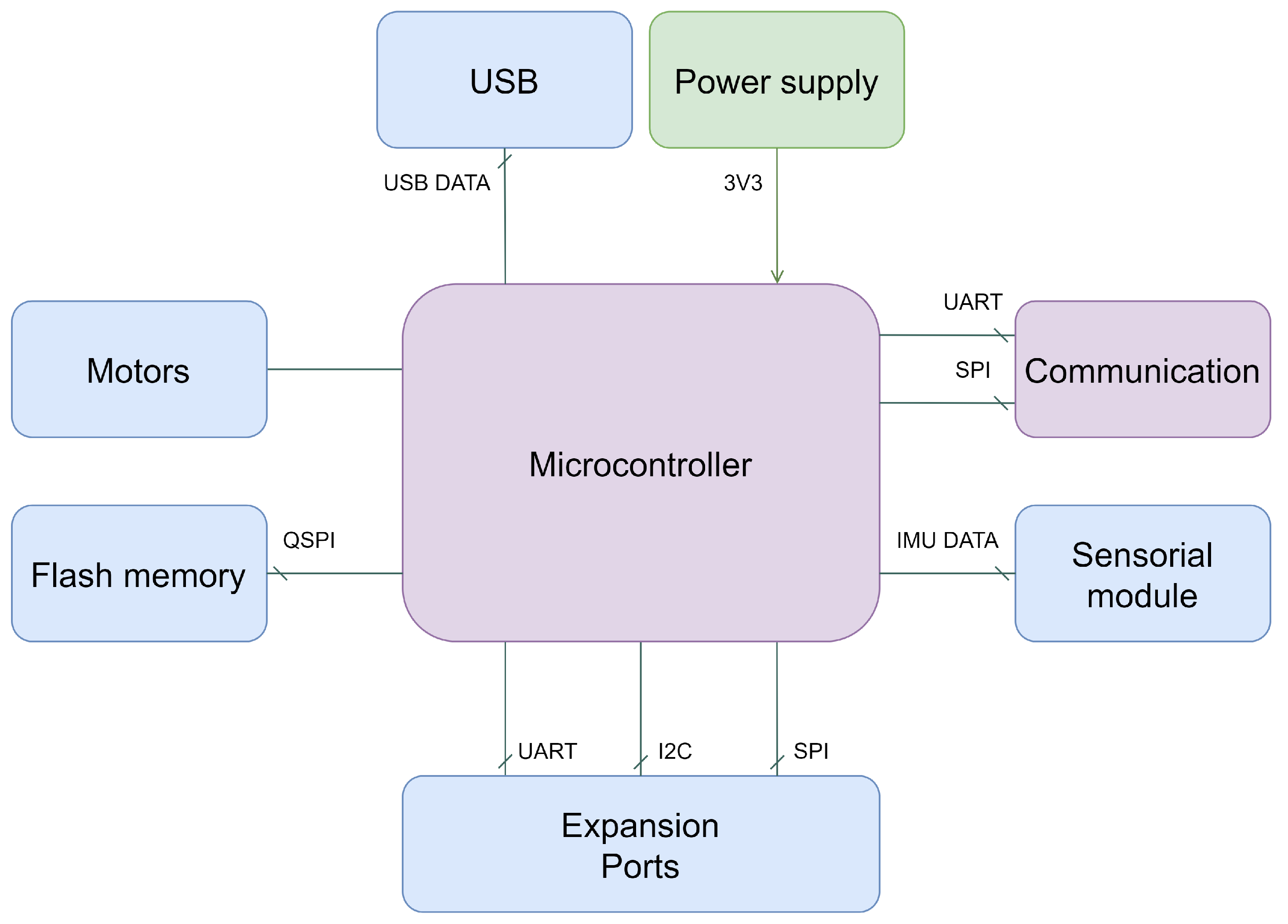
We divided the developed schematic into blocks for easier understanding. Figure 2 shows a high-level diagram of the NAB that demonstrates the fundamental blocks of the schematic and the communication between them. Since we used Crazyflie 2.1 as a starting point, this diagram represents the architecture of the schematic for the Crazyflie 2.1.

Figure 2. High-level diagram of the NAB.

To develop the schematic, we utilised EasyEDA (https://easyeda.com/, accessed on 27 March 2023) software with the existing library components because it is a free solution with online collaborative tools. EasyEDA enables the creation of original schematics and PCBs and displays the 3D visualisation of the designed boards.

Although we used Crazyflie 2.1 as the basis for developing the NAB, we made several significant changes. Table 2 shows the components of both NAVs for all blocks.

Table 2. Components in each block of Crazyflie 2.1 and NAB.

Block	Crazyflie 2.1	NAB
Microcontroller	STM32F405RG	RP2040
Communication	NRF51822	NINA-W106
	RFX2411N
Sensorial module	BMI088	BMI088
	BMP388	VL53L1X
Motors	4 × DC motors	5 × DC motors
USB	micro USB	micro USB
Flash Memory	24AA64FT-E/OT	W25Q128JVSIQ TR
Power supply	BQ24075	BQ24075
	LP29075	LDK130M33R
	NCP702SN30
	SIP32431

Below, we explain each block and the changes we made. To achieve this, we compared the schematic of the Crazyflie 2.1 with that of the developed NAB.

• Microcontroller

The microcontroller is the most important component in the architecture since it is impossible to control a vehicle without it. Changing this component can lead to more efficient and effective control of the NAB. We decided to replace the STM32F405RG with the RP2040.

The Raspberry Pi RP2040 is a microcontroller designed to achieve high performance. The distinguishing features of this microcontroller are its scalable on-chip memory, dual-core processor, and increased peripheral set. The RP2040 is a stateless device that supports cached execute-in-place commands from external QSPI memory. This allows it to choose the appropriate flash memory. The manufacturer of the RP2040 uses a 40 nm process node, providing high performance, low dynamic power consumption, and low leakage (https://datasheets.raspberrypi.com/rp2040/rp2040-datasheet.pdf, accessed on 27 March 2023).

In Table 3, we highlight some of the features of the RP2040 and STM32F405RG microcontrollers, which we used to perform a thorough comparison. The characteristics that show that the RP2040 has an advantage are highlighted in purple. On the other hand, the features that show that the STM32F405RG has an advantage are highlighted in green.

Table 3. RP2040 and STM32F405RG microcontroller characteristics.

Features	RP2040	STM32F405RG
Cores	Dual-core	Single-core
Core architecture	32-bit ARM Cortex-M0+	32-bit ARM Cortex-M4
CPU clock	Flexible clock up to 133 MHz	168 MHz
RAM size	264 KByte SRAM	up to 192 + 4 Kbytes SRAM
Flash size	up to 16 MByte external flash	up to 1 MByte external flash
MCU power voltage	3.3 VDC	3.3 VDC
GPIO	30	51
UART	2	2
I2C	2	3
SPI	2	3
Dimensions	7.75 × 7.75 mm	12.7 × 12.7 mm

The RP2040 is dual-core, allowing it to run processes in parallel and making its performance significantly better. On the other hand, the main disadvantage of the RP2040 is its ARM Cortex-M0+ because the ARM Cortex-M4 in the STM32F405RG is faster and more energy-efficient. By analysing the Crazyflie 2.1 schematic, we found that the RP2040 had the required number of pins to connect the components to the microcontroller. The fact that the RP2040 had fewer pins did not invalidate its utilisation in the schematic.

The determining characteristic for the choice was related to the dimensions of the components. Since the goal was to build a NAV, the board dimensions were limited; therefore, we selected the RP2040.

The RP2040 is a recent purpose-built device that provides high performance and low dynamic power consumption, which are essential features for a NAV. The RP2040 dual-core component allows the running of parallel tasks and achieves significantly better performance than the single-core STM32F405RG. Given the small dimensions of the NAV, we selected the RP2040, as it was only 7.75 × 7.75 mm, whereas the STM32F405RG measured 12.7 × 12.7 mm.

• Communication

Our goal was to develop a NAV capable of moving and pollinating autonomously. Communication is central in an autonomous vehicle so information about the surroundings is analysed and the NAV reacts in time.

The Crazyflie 2.1 uses the NRF51822 and RFX2411N as the core components of the communication module. This hardware provides low-latency/long-range radio communication and Low-Energy (LE) Bluetooth. However, as these components were not available due to the pandemic, it was necessary to find another way to communicate wirelessly.

The AI Deck 1.1 uses the NINA-W102 component to communicate via Wi-Fi. This component allows communication through various protocols. The only difference between the NINA-W102 and the NINA-W106 is the number of pins available. Since the NINA-W106 was the only one in stock, we chose this component.

We chose to incorporate the NINA-W106 into the schematic. This device has the following advantages: the ability to use different communication protocols and the fact that it does not require additional components to ensure operation.

The NINA-W106 is a standalone multi-radio MCU module consisting of a radio for wireless communication, an internal antenna, and a microcontroller. The radio supports Wi-Fi and Bluetooth communications. The NINA-W106 includes several components, making it a very compact standalone multi-radio module with dimensions of 10.0 × 14.0 × 2.2 mm (https://content.u-blox.com/sites/default/files/NINA-W10_DataSheet_UBX-17065507.pdf, accessed on 27 March 2023).

The purpose of the NAB is to pollinate flowers so flower detection is essential. By adding the NINA-W106, a user can stream the images collected by the NAB over Wi-Fi and run the detection and control code off-board. The NINA-W106 can use the same communication protocol as the Crazyflie 2.1 components, without the need for additional elements.

• Sensorial Module

The sensor module consists of an IMU and a distance sensor. The purpose of this module is to help in the navigation and control of the NAB.

The Crazyflie 2.1 has an IMU consisting of a gyroscope, accelerometer (BMI088), and pressure sensor (BMP388). The BMP388 enables accurate altitude tracking. Light Detection and Ranging (LiDAR) sensors can perform the pressure sensor function. We opted to use the VL53L1X (https://www.st.com/resource/en/datasheet/vl53l1x.pdf, accessed on 27 March 2023) and BMI088 (https://download.mikroe.com/documents/datasheets/BMI088_Datasheet.pdf, accessed on 27 March 2023).

The BMI088 is an IMU that combines a gyroscope and an accelerometer to detect movements and rotations. The VL53L1X is equipped with a Time-of-Flight (ToF) laser-ranging sensor that can accurately measure distances of up to 4 m and has a fast-ranging frequency of up to 50 Hz, regardless of the target’s colour and reflectance. This component is often used in drones to assist with flight.

By adding the VL53L1X component, we have upgraded the IMU module to a sensory module. In addition to the features of an IMU, with the VL53L1X, it is possible to measure the relative distance to the ground.

• Motors

The schematic developed in the motor block maintained the structure of the schematic of the Crazyflie 2.1. We chose to add a fifth motor with a vertical orientation. The aim was to directly allow forward movement without modifying the roll angle. Managing the direction of the NAV for flower pollination became more straightforward due to the fifth motor. The addition of the fifth motor resulted in enormous advantages for NAB control. 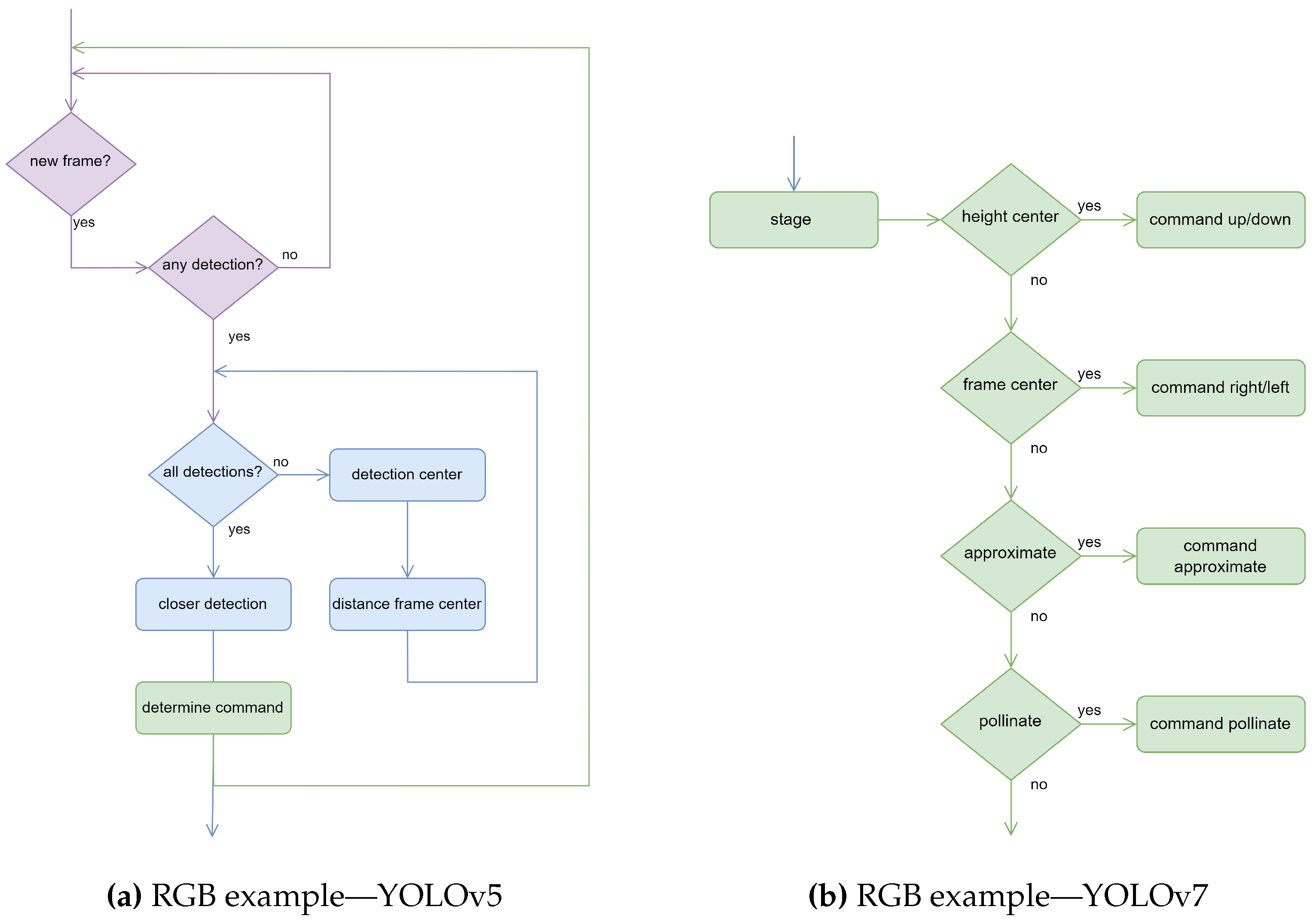As described in Section 4, after positioning the flower in the centre of the image, the NAB approached it to pollinate. To achieve this, it only needed to activate the fifth motor.

• Flash Memory

Flash memories are non-volatile memories that store information without an active power source and have several different characteristics. The 24AA64FT-E/OT flash memory (https://ww1.microchip.com/downloads/en/DeviceDoc/21189T.pdf, accessed on 27 March 2023) used in the Crazyflie 2.1 schematic was unavailable. Therefore, we chose to use the W25Q128JVSIQ TR (https://www.winbond.com/resource-files/w25q128jv%20revf%2003272018%20plus.pdf, accessed on 27 March 2023). Table 4 lists the various features of the memories mentioned above. The selected flash memory had more advantages and was appropriate for the system.

Table 4. W25Q128JVSIQ TR (https://www.winbond.com/resource-files/w25q128jv%20revf%2003272018%20plus.pdf, accessed on 27 March 2023) and 24AA64FT-E/OT (https://ww1.microchip.com/downloads/en/DeviceDoc/21189T.pdf, accessed on 27 March 2023) flash memories characteristics.

Features	W25Q128JVSIQ TR	24AA64FT-E/OT
Clock frequency (max)	133 MHz	400 kHz
Memory size	128 Mb (16 M × 8)	64 Kb (8 K × 8)
Write-cycle time	3 ms	5 ms
Access time (max)	6 ns	3500 ns
Supply voltage	2.7 V to 3.6 V	1.7 V to 5.5 V
Memory interface	QSPI, QPI, DTR	I2C

The flash memory selected for the NAB had better features such as a lower write-cycle time and maximum access time. In addition, it could connect to the RP2040 via the QSPI interface.

• Power supply

The power supply block contains components that regulate the voltage received via the USB port or the battery powering the NAB.

Eliminating the components of the communication block of the Crazyflie 2.1 schematic reduced the number of integrators required in the power supply block. The function of the NCP702SN30 is to regulate the voltage to the nRF51822. Therefore, we removed that component. We also eliminated the SIP32431 element, as the output signal powers some optional shields on the Crazyflie 2.1. We did not need this element in the NAB. The NAB schematic maintained the BQ24075 (https://www.ti.com/lit/ds/slusau3b/slusau3b.pdf?ts=1656253857759&ref_url=https%253A%252F%252Fwww.google.com%252F, accessed on 27 March 2023) and LP2985 (https://www.ti.com/lit/ds/symlink/lp2985a.pdf?ts=1656282441972&ref_url=https%253A%252F%252Fwww.google.com%252F, accessed on 27 March 2023) components.

The BQ24075 is the most critical component of this power pack, as it regulates the system power supply (USB or battery). The device powers the system while independently charging the battery. The power input source for charging the battery is a USB port, connected via a VUSB signal. Furthermore, the nRF51822 controls the BQ24075 in the Crazyflie 2.1 schematic.

The LP2985 is a low-dropout (LDO) regulator with an output current capability of 150 mA continuous load current. This component is available in many voltages. Since $3.3$ V powers the system, the LP2985A-33DBVR circuit was chosen, which can regulate the voltage up to $3.3$ V. The VCC signal is $3.3$ V and supplies the integrated microcontroller and communication blocks. The VCCA signal is the filtered VCC signal, which results in analogue power that is only used by the sensorial module block.

Table 5 shows the minimum and maximum consumption of the components supplied by the LP2985A-33DBVR regulator, highlighted in green. By analysing the consumption, it was found that the LP2985A-33DBVR regulator was unsuitable, given that the NINA-W106 consumes 627 mW and the LP2985A-33DBVR provides a maximum of 495 mW.

Table 5. Component consumption and power supplied by the LP2985A-33DBVR regulator.

Component	V	Imin	Pmin	Imax	Pmax
RP2040	3.3 V	0.18 mA	0.594 mW	35.5 mA	117.15 mW
NINA-W106	3.3 V	0.005 mA	0.0165 mW	190 mA	627 mW
BMI088 accelerometer	3.3 V	0.003 mA	0.0099 mW	0.150 mA	0.495 mW
BMI088 gyroscope	3.3 V	0.025 mA	0.0825 mW	5 mA	16.5 mW
VL53L1X	3.3 V	0.003 mA	0.0099 mW	18 mA	59.4 mW
LP2985A-33DBVR	3.3 V	1 mA	3.3 mW	150 mA	495 mW

The total consumption of the components powered by the regulator is $820.545$ mW so we need a regulator that provides power equal to or greater than $820.545$ mW. A higher current is required, as the voltage must be 3.3 V. The LDK130M33R (https://www.st.com/resource/en/datasheet/ldk130.pdf, accessed on 27 March 2023) meets all the criteria (provides a maximum of 990 mW, which is higher than 820 mW) and is very similar to the LP2985A-33DBVR. Table 6 shows the values of the new voltage regulator, which are highlighted in green.

Table 6. Component consumption and power supplied by the LDK130M33R regulator.

Component	V	Imin	Pmin	Imax	Pmax
RP2040	3.3 V	0.18 mA	0.594 mW	35.5 mA	117.15 mW
NINA-W106	3.3 V	0.005 mA	0.0165 mW	190 mA	627 mW
BMI088 accelerometer	3.3 V	0.003 mA	0.0099 mW	0.150 mA	0.495 mW
BMI088 gyroscope	3.3 V	0.025 mA	0.0825 mW	5 mA	16.5 mW
VL53L1X	3.3 V	0.003 mA	0.0099 mW	18 mA	59.4 mW
LDK130M33R	3.3 V	-	-	300 mA	990 mW

Table 7 shows the consumption of all the components used in the NAB. In this case, the LiPo 25 mAh battery is the system’s power supply and its values are highlighted in green; the values of the LDK130M33R regulator are shown for the consumer. For the values that refer to the battery (https://store.bitcraze.io/collections/spare-parts/products/250mah-lipo-battery-including-500ma-usb-charger, accessed on 27 March 2023) and motors (https://www.bitcraze.io/documentation/hardware/motor_7mm/motor_7mm-datasheet.pdf, accessed on 27 March 2023), we used the same components as the Crazyflie 2.1. The total maximum consumption of the system was calculated by summing the maximum consumption of all the elements listed in Table 7. Note that the NAB uses five motors so to calculate the total consumption, we multiplied the motor consumption by five. The value of the total maximum consumption of the designed NAB is $21.919$ W.

Table 7. Component consumption and power supplied by the LiPo battery.

Component	V	Imin	Pmin	Imax	Pmax
RP2040	3.3 V	0.18 mA	0.594 mW	35.5 mA	117.15 mW
NINA-W106	3.3 V	0.005 mA	0.0165 mW	190 mA	627 mW
BMI088 accelerometer	3.3 V	0.003 mA	0.0099 mW	0.150 mA	0.495 mW
BMI088 gyroscope	3.3 V	0.025 mA	0.0825 mW	5 mA	16.5 mW
VL53L1X	3.3 V	0.003 mA	0.0099 mW	18 mA	59.4 mW
LDK130M33R	0.1 V	-	-	100 mA	10 mW
BQ24075	3.7 V	0.0043 mA	0.0159 mW	1.5 mA	5.55 mW
DC motor	4.2 V	-	-	1000 mA	4200 mW
W25Q128JV	3.3 V	0.001 mA	0.0033 mW	25 mA	82.5 mW
LiPo battery	3.7 V	-	-	3750 mA	13,875 mW

The developed schematic is similar to Crazyflie 2.1 schematic. We eliminated the NCP702SN30, SIP32431, and LP29075 components and added the LDK130M33R regulator, thereby decreasing the number of connections and elements on the NAB board.

This block underwent many changes that reduced the number of components and connections, which was its most significant advantage, given the dimensions of a NAV. The changes were made due to the power consumed by the introduced components. The operation of this block is identical in both NAVs.

3.1.2. Printed Circuit Board

For the design of a PCB for a NAB, it is crucial to perform the following steps to minimise the length of the tracks:

• Determine the PCB structure;
• Study and place the components and define the PCB layout;
• Analyse and make connections between components.

After defining the NAB schematic, we began work on the PCB design. The shape and dimensions of the PCB are similar to those of the Crazyflie 2.1 to ensure aerodynamics. The board consists of a 30 × 30 mm square with some arms at each vertex of 20 × 7 mm. As with the AI Deck 1.1, we added a small platform for the NINA-W106 (12.7 × 8 mm).

Board mapping was analysed to minimise track length. In particular, the following constraints in terms of the level of orientation and/or the position of each element on the board were considered:

• Since the RP2040 is connected to the highest number of components, the microcontroller should be in the centre of the board. Additionally, it is crucial to avoid placing any elements that could interfere with vias in the opposite layer.
• The voltage decoupling capacitors must be placed close to the RP2040 power supply pins to reduce noise.
• The NINA-W106 must be in the top layer, given the size and weight of the component.
• The micro USB connector must be on the top layer, closer to the edge, and oriented for easy access.
• The 8-pin connectors must be on the sides of the board. None of these sides must coincide with the micro USB connector.
• Four motors must be at each end of the arms so the corresponding connectors must be at the start (by arms, we mean the rectangular platforms of the board).
• The fifth motor must be on the edge of the board.
• The VL53L1X must be on the bottom layer to measure the distance to the ground.
• The buttons of the flash memory must be on the top layer for easy access.

In addition, it is crucial to check the pinout of the RP2040 to place the other components accordingly. A board layout that minimises track length based on the RP2040 pinout was studied, along with the previously mentioned constraints. To ensure the NAB was balanced and the connections between components could be easily made, we carefully considered the weight distribution and orientation of the components when placing them on the PCB.

Additionally, different track specifications were considered when tracing the connections, namely:

• For the connections of the microcontroller, it was necessary to use tracks with a width of 9 mil so that there was no contact between pins.
• Most of the links were 10 mil wide.
• The motor tracks were 14 mil wide to facilitate heat dissipation.

To facilitate communication between the different layers, we utilised vias—small holes that establish electrical connections—between all layers, with a diameter of 24 mil and a drilling diameter of 12 mil.

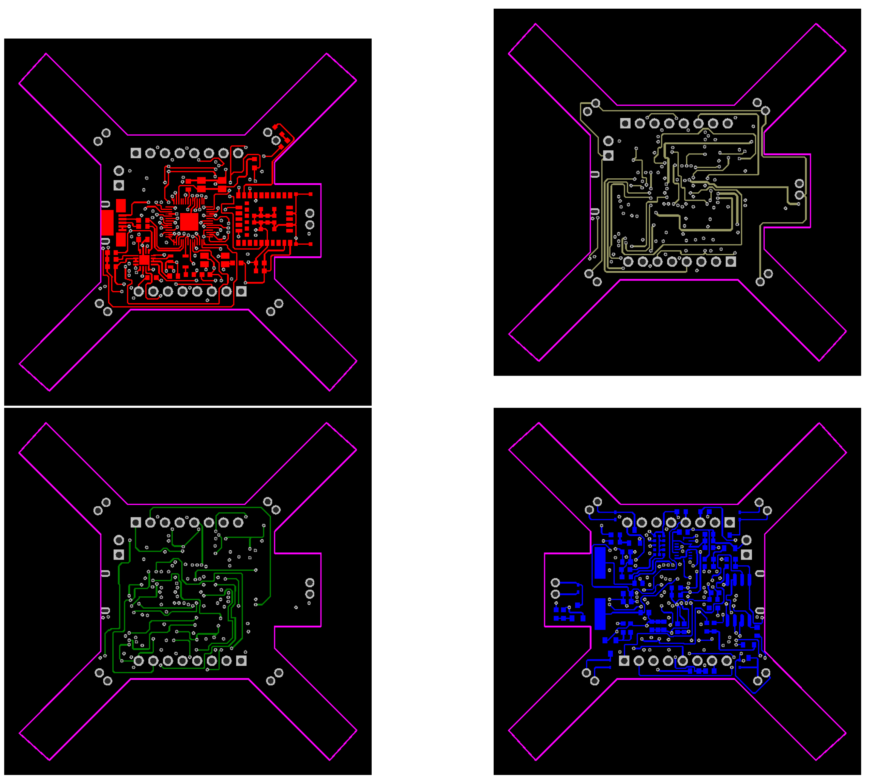
Figure 3 shows the components and connections of each layer. The upper and lower layers are the most populated. The wider tracks related to the motors are in the inner 1 layer.

Figure 3. The four layers of the NAB’s PCB. (1) Top layer. (2) Inner 1 layer. (3) Inner 2 layer. (4) Bottom layer.

The development of the NAB’s PCB presented many challenges due to the reduced board size that contained many components and increased connections.

3.2. Software

Since the NAB’s goal is pollination, it must be able to recognise flowers and execute commands to approach them. Identification is possible using perception algorithms to process the images a camera acquires. For this purpose, it is necessary to develop a Deep Learning Neural Network (DLNN) for flower recognition and implement an algorithm that defines the command to be executed by the NAB based on the position of the flower detected in the frame. From data collection to autonomous flower detection, three steps were performed:

• Data collection: collecting and storing images to build the input dataset;
• Dataset generation: annotating images by drawing bounding boxes around the flowers;
• Model training: training the DL models to be deployed in the NAV for real-time flower detection.

3.2.1. Data Collection

For the flower detection process, it was necessary to build a new dataset. We utilised the Flower Detection Dataset (https://doi.org/10.5281/zenodo.7560779, accessed on 27 March 2023) that contained images taken using an iPhone XR of a group of eight flowers from various perspectives (https://www.gsmarena.com/apple_iphone_xr-9320.php, accessed on 27 March 2023). The images with a 4032 × 3024 resolution were taken from various distances while moving around the flowers. A total of 103 images were collected and Figure 4 shows some examples of the photographs taken from different perspectives and distances.

Figure 4. Sample images from the dataset.

3.2.2. Dataset Generation

The dataset generation was performed using the collected data to form the DL models. Since a supervised learning approach was used, the models required the annotation of each input image. Each annotation contained a bounding box around each object, representing its area, position, and class.

Computer Vision Annotation Tool (CVAT) software (https://github.com/openvinotoolkit/cvat, accessed on 27 March 2023) was used to perform the manual annotations by only considering the class “flower”. In this process, 499 flowers were identified in the collected dataset. The images were exported under the YOLO [34] format to train the YOLO models.

Since the AI Deck 1.1 module can use an RGB or grayscale camera with a resolution of 320 × 320 pixels, an image-processing step was performed after annotation. First, the images were resized from 4608 × 2592 to 320 × 240 pixels. Figure 5 shows some examples of the resized images with a resolution of 320 × 240.

Figure 5. Sample resized images from the dataset.

Next, the dataset was duplicated by converting the images from RGB to grayscale. The conversion of the RGB images to grayscale while maintaining the three input channels was performed using a Python script, without the need to change the network architecture. Figure 6 shows some examples of grayscale images with a resolution of 320 × 240.

Figure 6. Sample grayscale images from the dataset.

The Flower Detection dataset containing 206 images (RGB and grayscale images) was divided into three sets: training (60%) with 126 images, validation (20%) with 40 images, and test (20%) with 40 images. This dataset containing 206 annotations and (RGB and grayscale) images of flowers with a resolution of 320 × 240 is available at https://doi.org/10.5281/zenodo.7708820, accessed on 23 January 2023.

3.2.3. Model Training

The final step was the training and deployment of the models. The YOLO models (YOLOv5, YOLOv7, and YOLOR) were trained using Pytorch. For each model, we chose the smaller version. Table 8 shows the characteristics of each selected version.

Table 8. Performance of YOLO versions.

Model	mAP 50	AP 50	Speed
	Validation Set	Testing Set	Batch Size 32
YOLOv5n	45.7%	-	0.6 ms
YOLOv7	-	69.7%	2.8 ms
YOLOR-CSP	-	71.2%	3.2 ms

Each model was trained individually on the Flower Detection Dataset for 300 epochs with a batch size of 64 images and an input resolution of 320 × 320 pixels using an NVIDIA GeForce 3090 Graphics Processing Unit (GPU) with 32 GigaBytes (GB) of available memory. Each training used the pre-trained weights and configuration provided by the YOLO developers.

4. Results

4.1. Methodology

The selection of appropriate metrics to evaluate deep learning models depends on the specific problem at hand. Metrics offer distinct perspectives on the performance of a deep learning model and are often used in combination to gain a comprehensive understanding of its behaviour. The metrics listed below are commonly used to evaluate the outcomes of object detection and classification.

To determine the type of detection, it is necessary to understand the differences between a “correct detection” and an “incorrect detection”. One way is to use the intersection over union (IoU).

Intersection over Union (IoU) is based on the Jaccard Index, which measures the similarity coefficient for two datasets. In this paper, the IoU is used to measure the area of overlap between two bounding boxes using the ground-truth and predicted bounding boxes.

We can classify a detection as valid or invalid by comparing the IoU with a given threshold t. If the IoU $\ge t$, the detection is considered valid and if the IoU $<t$, it is considered invalid. To determine the types of detections, we utilised the concepts defined below:

• True Positive (TP): A valid detection of a ground-truth bounding box, i.e., IoU $\ge t$;
• False Positive (FP): An invalid detection (incorrect detection of a non-existent object or incorrect detection of a ground-truth bounding box), i.e., IoU $<t$;
• False Negative (FN): An invalid detection of a ground-truth bounding box;
• True Negative (TN): Not applicable in object detection. There is no need to find infinite bounding boxes in each image during object detection.

The evaluation of the object detection methods mainly involved the concepts of precision and recall:

• Accuracy calculates the ratio of the number of correct predictions to the total number of predictions:

  $$Accuracy=\frac{TP+TN}{TP+TN+FP+FN}$$

  (1)
• Precision measures the ability of the model to identify only the relevant objects, i.e., the percentage of valid detections out of all detections and is calculated by:

  $$Precision=\frac{TP}{TP+FP}$$

  (2)
• Recall measures the ability of the model to find all ground-truth bounding boxes, i.e., the percentage of valid detections out of all ground truths and is calculated by:

  $$Recall=\frac{TP}{TP+FN}$$

  (3)
• F1 score represents the harmonic mean between precision and recall and is used to evaluate performance; it is calculated by:

  $$F1score=2\ast \frac{Precision\ast Recall}{Precision+Recall}$$

  (4)

The precision × recall curve is a way to evaluate the performance of an object detector. This procedure plots a curve as confidence changes for each object class. A good object detector maintains high precision as recall increases. In other words, by varying the confidence threshold, precision and recall should remain high. A poor object detector for recovering all ground-truth objects (increasing recall) needs to increase the number of detected objects (increasing FP, which implies decreasing precision) to retrieve all ground-truth objects (high recall). Therefore, an optimal detector identifies only the relevant objects (FP = 0, indicating high precision) while finding all ground-truth objects (FN = 0, implying high recall).

The Average Precision (AP) is another way to evaluate the quality of the object detector. AP compares the performance of object detectors to calculate the area under the precision × recall curve. AP is the average precision of all recall values between 0 and 1. Therefore, a high area represents both high precision and recall.

The mean Average Precision (mAP) is a metric used to measure the accuracy of object detectors across all classes. The mAP is the average AP across all classes. In this case, mAP and AP represent the same value since only one class exists.

4.2. Evaluation

To evaluate the Flower Detection Dataset, the validation set results were generated using an exact input resolution of 320 × 320 with a batch size of 64. Additionally, an IoU threshold of 50% was considered. Table 9 shows the confidence threshold value that maximised the F1 score for each model in the validation set.

Table 9. Confidence threshold values that optimised the F1 score for each YOLO.

Model	Confidence Threshold	F1 Score
YOLOv5	71%	94%
YOLOv7	70%	96%
YOLOR	69%	97%

The confidence threshold values presented led to the best balance between precision and recall, which maximised the number of true positives and minimised the number of false positives and false negatives. All three models had similar confidence threshold values and similar confidence in their predictions.

Table 10 shows the results of the test set. The inference was performed for a 0% confidence threshold and the confidence threshold value that maximised the F1 scores in the validation set. The inference was performed with a batch size of 8 and an IoU threshold of 50 %. In the test set, a batch size of 8 was used, as the processing capacity was smaller.

Table 10. Detection results of the testing set obtained from the Flower Detection Dataset.

Model	Confidence Threshold	Accuracy	Precision	Recall	F1 Score	mAP	Time per Image
YOLOv5	>0%	25%	25%	99%	40%	71%	1.9 ms
	71%	92%	97%	95%	96%	69%	2.0 ms
YOLOv7	>0%	15%	15%	100%	26%	81%	3.4 ms
	70%	97%	98%	99 %	98%	80%	2.3 ms
YOLOR	>0%	44%	44%	99%	61%	82%	4.6 ms
	69%	97%	98%	99%	98%	81%	2.7 ms

Lower confidence rates typically lead to an increase in false positives and a decrease in false negatives. As a result, precision decreases due to the increase in false positives and recall increases due to the decrease in false negatives. The results show that limiting the confidence threshold of the models resulted in a considerable increase in accuracy, precision, and F1 score at the cost of a slight decrease in recall and mAP. When the confidence threshold is set to maximise accuracy, precision and F1 score remain in the range of 90% to 99%.

Figure 7 shows two images (grayscale and RGB) from the test set and the ability of the models to detect flowers.

Figure 7. Detection of flowers in sample images from the test set of the Flower Detection Dataset. (a–c) RGB example and (d–f) grayscale example. Orange bounding boxes present ground truth. Light green bounding boxes present the predictions from YOLOv5. Dark green bounding boxes present the predictions from YOLOv7. Blue bounding boxes present the predictions from YOLOR.

The three models achieved outstanding performance in the detection of flowers, even at a resolution of 320 × 240 pixels. The models successfully detected flowers in the RGB and grayscale images. These results demonstrate the robustness of the model and its ability to successfully handle different scenarios.

The Flower Detection Dataset was designed to detect one type of flower. The three trained networks were tested on a public dataset to evaluate the robustness of the three trained models. In the literature, there are many datasets that are only used for classification and do not have annotations. The TensorFlow Flower Dataset is a public open-access flower dataset used for classification that contains images characterised by distinct flower types, backgrounds, and resolutions. The TensorFlow Flower Detection Dataset (https://www.tensorflow.org/datasets/catalog/tf_flowers, accessed on 23 March 2023) contains the same images and associated annotations in a YOLO format, which can be utilised for flower detection. We used CVAT software to annotate more than 3500 images, which resulted in more than 14,000 bounding boxes.

Table 11 shows the results obtained from the TensorFlow Flower Detection Dataset using each trained model. The inference was performed with a 0% confidence threshold, which can maximise the F1 scores. The inference was performed with a batch size of 8 and an IoU threshold of 50%.

Table 11. Detection results obtained from the TensorFlow Flower Detection Dataset.

Model	Confidence Threshold	Accuracy	Precision	Recall	F1 score	mAP	Time per Image
YOLOv5	>0%	3%	3%	68%	5%	12%	1.1 ms
	71%	13%	69%	14%	23%	6%	0.9 ms
YOLOv7	>0%	1%	1%	70%	2%	12%	1.8 ms
	70%	11%	64%	12 %	21%	5%	1.4 ms
YOLOR	>0%	3%	3%	66%	6%	18%	2.4 ms
	69%	20%	67%	22%	33%	11%	2.2 ms

As we can see in Table 11, when the confidence ratio was greater than zero, there was a decrease in accuracy (increase in FP) and an increase in recall (decrease in FN). As the Flower Detection Dataset was only trained for one flower type, the values of the metrics decreased. By assuming the confidence threshold value that maximises the F1 score, the values of the metrics stabilised at around the same values. Precision was the best-performing metric for the three models when the confidence threshold maximised the F1 score, which means that there were more FNs than FPs.

To better understand the results obtained with the Flower Detection Dataset, we decided to train the three YOLO models with the TensorFlow Flower Detection Dataset. As before, the training was performed for each model individually for 300 epochs with a batch size of 64 images and an input resolution of 320 × 320 pixels using an NVIDIA GeForce 3090 Graphics Processing Unit (GPU) with 32 GigaBytes (GB) of available memory. It was also chosen so we could use the pre-trained weights and configuration provided by the YOLO developers.

The results of the validation set were generated using an exact input resolution of 320 × 320 with a batch size of 64 and an IoU threshold of 50%. Table 12 shows the confidence threshold values that maximised the F1 score for each model in the validation set.

Table 12. Confidence threshold values that optimised the F1 score obtained with the TensorFlow Flower Detection Dataset.

Model	Confidence Threshold	F1 Score
YOLOv5	56%	80%
YOLOv7	75%	80%
YOLOR	73%	82%

This value represented the best balance between precision and recall, which maximised the number of true positives and minimised the number of false positives and false negatives. All three models had similar confidence threshold values and similar confidence in their predictions.

Table 13 shows the results of the test set. The inference was performed for a 0% confidence threshold and the confidence threshold value that maximised the F1 scores in the validation set. The inference was performed with a batch size of 8, as the processing capacity was smaller, and an IoU threshold of 50%.

Table 13. Detection results of the testing set obtained with the TensorFlow Flower Detection Dataset.

Model	Confidence Threshold	Accuracy	Precision	Recall	F1 Score	mAP	Time per Image
YOLOv5	>0%	6%	6%	98%	12%	63%	1.2 ms
	56%	67%	83%	78%	81%	56%	1.1 ms
YOLOv7	>0%	7%	7%	99%	14%	67%	2.1 ms
	75%	68%	87%	76 %	81%	57%	2.0 ms
YOLOR	>0%	24%	24%	95%	38%	67%	2.4 ms
	73%	69%	84%	80%	82%	62%	2.4 ms

Similar to the Flower Detection Dataset, the results indicate that this approach is only applicable for mAP comparison and not for practical use, as the results for a confidence threshold greater than 0% are not meaningful. A recall value higher than or equal to 95% indicates that quite a few flowers were detected and correctly classified according to the bunch conditions. However, a precision value lower than 25% indicates that there were quite a few incorrect detections of flowers, which were also expected to have a low F1 score value.

Assuming the confidence threshold value that maximises the F1 score, there was a considerable increase in precision and F1 score, albeit at the cost of a slight decrease in recall and mAP. The precision values were above 80%, indicating that the models sometimes made incorrect detections. However, a higher number of flowers were missed. An F1 score above 80% demonstrates that the balance between precision and recall was much higher, whereas the mAP value barely changed with the threshold change.

Overall, the results for the three models are promising and similar. YOLOR achieved the best performance in most metrics. To better understand the outcomes of some of the metrics it was necessary to observe the model detections on the test set images. Figure 8 presents the results of the ability of each YOLO version to detect grape bunches in a test set image. The models had good responses despite the complexity of the image, i.e., flowers of different sizes, overlapping, and with lower resolution.

Figure 8. Detection of flowers in samples from the test set of the TensorFlow Flower Detection Dataset. Orange bounding boxes present ground truth. (a) Light-green bounding boxes indicate the predictions from YOLOv5. (b) Dark-green bounding boxes indicate the predictions from YOLOv7. (c) Blue bounding boxes indicate the predictions from YOLOR.

The three models had outstanding responses in the detection of distinct types of flowers in different scenarios and at different resolutions. These results demonstrate the robustness of the trained models and their ability to successfully handle different scenarios.

Discussion

In this work, we created the Flower Detection Dataset by collecting an original dataset of flower images and generating additional data to expand the dataset. The YOLOv5n, YOLOv7, and YOLOR-CSP models were used for training and testing. It should be noted that the batch size was reduced for the test.

The results of the test set of the Flower Detection Dataset were satisfactory in the detection of flowers when using a confidence threshold that maximised the F1 score in the validation set. This was an essential step as it harmonised the results of the metrics and decreased the number of false positives. All models showed satisfactory results, with YOLOv7 and YOLOR achieving the best performances.

The models trained on the Flower Detection Dataset were also tested on the TensorFlow Flower Detection Dataset to assess robustness. As expected, the results of the metrics did not reach the same range of values. To verify the quality of the results achieved, the three models were trained again but this time on the TensorFlow Flower Detection Dataset, which had a greater variability of information. The results verified that a dataset with greater variability of information can lead to better performance. Therefore, it is important to invest in developing robust datasets with images of flowers of various species and different scenarios to improve the performance of deep learning models.

4.3. Control

The pollination task requires a complex algorithm that controls the flight of the NAB towards a flower. We added a camera to take photos of the surroundings of the NAB. For the NAB to recognise at least one flower, the algorithm must determine the closest flower to the centre of the image and guide the NAB to the selected flower.

The developed script is available at https://gitlab.inesctec.pt/agrob/NAB and includes the neural network trained to recognise flowers. We developed software that identifies the command that the NAB should follow to efficiently approach and pollinate a flower.

The algorithm analyses each frame and acts according to the information it has collected so far. To begin with, the algorithm checks the detections in each frame. If there are flower detections, the algorithm must calculate the centre of each detection and its distance to the centre of the frame. After performing the calculations for all detections, the algorithm determines the area that is closest to the centre of the image. Finally, the command that the NAB should follow is determined. Figure 9 shows a flowchart of the script.

Figure 9. Flowcharts of the flight-control of the NAB. (a) Flowchart of the flight control algorithm according to the recognition of flowers in the pollination phase. (b) Flowchart of the stages to define the command.

The algorithm defines the command to execute according to the active stage presented in Figure 9. Once the detection closest to the centre of the frame is defined, it is necessary to determine the command. The first goal is to place the flower in the centre of the height of the frame. The algorithm determines whether the NAB should move up or down to place the flower in the centre of the image height. When it reaches the centre of the height, the algorithm positions the flower in the middle of the frame, i.e., the centre. This way, whether the NAB should move to the left or right is defined. Upon reaching the centre, the NAB should move closer to the flower until the bounding box fills 50% of the image area. If the NAB is already close to the flower, it should proceed with pollination.

5. Conclusions

The development of a NAV is particularly challenging given the weight and wingspan limitations. A careful literature review analysis is crucial to determine the hardware to use. State-of-the-art of NAVs are expanding in popularity but are still underutilised. All articles examined used the Crazyflie 2.0 platform as a starting point.

Developing a hardware prototype is quite a complex task given the interactions between the hardware components. To design the NAB schematic, we analysed the Crazyflie 2.1 schematic and made some changes to make the NAB more efficient for pollination. Developing the PCB of the NAB was quite challenging because it was a small board with many components, indicating many connections.

At the software level, three YOLO models were tested for flower detection. To make the images in the dataset similar to those displayed in the AI deck, the resolution was reduced to 320 × 240, making flower detection more difficult. The training was performed with the lighter version of each model with a batch size of 16 and 300 epochs. In the test set, a batch size of 8 was used, as the processing capacity was smaller. All models demonstrated satisfactory results. YOLOv7 and YOLOR achieved the best performances.

The Flower Detection Dataset was developed to detect one type of flower. To evaluate the robustness of the three YOLO models trained on the Flower Detection Dataset, a public dataset (TensorFlow Flower Dataset) was selected and annotated to test the performance. The annotations are publicly available in the TensorFlow Flower Detection Dataset in a YOLO format that can be utilised for flower detection. The results verified that a dataset with higher variability of information leads to better performance. Investing in the development of a more robust dataset with images of flowers of various species and different scenarios could lead to better performance.

Furthermore, an algorithm that can define the command to be executed by the NAB based on the position of the flower detected in the frame was implemented. The developed software was tested on videos recorded with a smartphone that mimicked the flight of the NAB, and the commands that the NAB would execute were printed on the video. However, it would be necessary to add a camera to the NAB to test the script in an authentic context.

As for future work, there are several crucial points for the development and testing of the NAB. The main directions for future works are as follows:

• The study, development, and integration of an instrument for pollination into the NAB [35];
• The development of the NAB and its application in a real context for field testing;
• Investing in the development of a more robust dataset with images of flowers of various species and backgrounds;
• The study and comparison of deformable convolution and an attention mechanism to show that these computer vision operations can improve the detection performance of the detector [36,37];
• The analysis and implementation of NAB swarms to reduce the cost of pollination.

References

1. EFSA. Bee Health. 2021. Available online: https://www.efsa.europa.eu/en/topics/topic/bee-health (accessed on 27 December 2021).
2. van der Sluijs, J.P.; Vaage, N.S. Pollinators and global food security: The need for holistic global stewardship. Food Ethics 2016, 1, 75–91. [Google Scholar] [CrossRef]
3. Abou-Shaara, H.F. The foraging behaviour of honey bees, Apis mellifera: A review. Vet. Med. 2014, 59, 1–10. [Google Scholar] [CrossRef]
4. Hassanalian, M.; Abdelkefi, A. Classifications, applications, and design challenges of drones: A review. Prog. Aerosp. Sci. 2017, 91, 99–131. [Google Scholar] [CrossRef]
5. Franklin, E. Robot Bees vs. Real Bees—Why Tiny Drones Can’t Compete with the Real Thing. 2017. Available online: https://theconversation.com/robot-bees-vs-real-bees-why-tiny-drones-cant-compete-with-the-real-thing-72769 (accessed on 17 February 2022).
6. Institute, W. RoboBees: Autonomous Flying Microrobots. 2019. Available online: https://wyss.harvard.edu/technology/robobees-autonomous-flying-microrobots/ (accessed on 17 February 2022).
7. Potenza, A. Bee Optimistic: This Drone Can Still Pollinate Plants even If All the Bees Die. 2017. Available online: https://www.theverge.com/2017/2/9/14549786/drone-bees-artificial-pollinators-colony-collapse-disorder (accessed on 17 February 2022).
8. Redmon, J.; Divvala, S.; Girshick, R.; Farhadi, A. You only look once: Unified, real-time object detection. In Proceedings of the IEEE Conference on Computer Vision and Pattern Recognition, Las Vegas, NV, USA, 1–26 June 2016; pp. 779–788. [Google Scholar]
9. Wang, C.Y.; Bochkovskiy, A.; Liao, H.Y.M. YOLOv7: Trainable bag-of-freebies sets new state-of-the-art for real-time object detectors. arXiv 2022, arXiv:2207.02696. [Google Scholar]
10. Wang, C.Y.; Yeh, I.H.; Liao, H.Y.M. You only learn one representation: Unified network for multiple tasks. arXiv 2021, arXiv:2105.04206. [Google Scholar]
11. Wang, D.; Liu, Z.; Gu, X.; Wu, W.; Chen, Y.; Wang, L. Automatic detection of pothole distress in asphalt pavement using improved convolutional neural networks. Remote Sens. 2022, 14, 3892. [Google Scholar] [CrossRef]
12. Liu, Z.; Gu, X.; Chen, J.; Wang, D.; Chen, Y.; Wang, L. Automatic recognition of pavement cracks from combined GPR B-scan and C-scan images using multiscale feature fusion deep neural networks. Autom. Constr. 2023, 146, 104698. [Google Scholar] [CrossRef]
13. Bučko, B.; Lieskovská, E.; Zábovská, K.; Zábovskỳ, M. Computer Vision Based Pothole Detection under Challenging Conditions. Sensors 2022, 22, 8878. [Google Scholar] [CrossRef]
14. Huang, Z.; Li, Y.; Zhao, T.; Ying, P.; Fan, Y.; Li, J. Infusion port level detection for intravenous infusion based on Yolo v3 neural network. Math. Biosci. Eng. 2021, 18, 3491–3501. [Google Scholar] [CrossRef]
15. Gallo, I.; Rehman, A.U.; Dehkordi, R.H.; Landro, N.; La Grassa, R.; Boschetti, M. Deep Object Detection of Crop Weeds: Performance of YOLOv7 on a Real Case Dataset from UAV Images. Remote Sens. 2023, 15, 539. [Google Scholar] [CrossRef]
16. Liu, Q.; Zhang, Y.; Yang, G. Small unopened cotton boll counting by detection with MRF-YOLO in the wild. Comput. Electron. Agric. 2023, 204, 107576. [Google Scholar] [CrossRef]
17. Ahmad, I.; Yang, Y.; Yue, Y.; Ye, C.; Hassan, M.; Cheng, X.; Wu, Y.; Zhang, Y. Deep learning based detector YOLOv5 for identifying insect pests. Appl. Sci. 2022, 12, 10167. [Google Scholar] [CrossRef]
18. Li, K.; Zhai, L.; Pan, H.; Shi, Y.; Ding, X.; Cui, Y. Identification of the operating position and orientation of a robotic kiwifruit pollinator. Biosyst. Eng. 2022, 222, 29–44. [Google Scholar] [CrossRef]
19. Tacconi, G.; Michelotti, V.; Cacioppo, O.; Vittone, G. Kiwifruit pollination: The interaction between pollen quality, pollination systems and flowering stage. J. Berry Res. 2016, 6, 417–426. [Google Scholar] [CrossRef]
20. Li, K.; Huo, Y.; Liu, Y.; Shi, Y.; He, Z.; Cui, Y. Design of a lightweight robotic arm for kiwifruit pollination. Comput. Electron. Agric. 2022, 198, 107114. [Google Scholar] [CrossRef]
21. Lim, J.; Ahn, H.S.; Nejati, M.; Bell, J.; Williams, H.; MacDonald, B.A. Deep neural network based real-time kiwi fruit flower detection in an orchard environment. arXiv 2020, arXiv:2006.04343. [Google Scholar]
22. Mu, X.; He, L.; Heinemann, P.; Schupp, J.; Karkee, M. Mask R-CNN based apple flower detection and king flower identification for precision pollination. Smart Agric. Technol. 2023, 4, 100151. [Google Scholar] [CrossRef]
23. Li, G.; Fu, L.; Gao, C.; Fang, W.; Zhao, G.; Shi, F.; Dhupia, J.; Zhao, K.; Li, R.; Cui, Y. Multi-class detection of kiwifruit flower and its distribution identification in orchard based on YOLOv5l and Euclidean distance. Comput. Electron. Agric. 2022, 201, 107342. [Google Scholar] [CrossRef]
24. Hulens, D.; Van Ranst, W.; Cao, Y.; Goedemé, T. Autonomous Visual Navigation for a Flower Pollination Drone. Machines 2022, 10, 364. [Google Scholar] [CrossRef]
25. Fan, H.; Yang, M.; Wang, R.; Wang, X.; Yue, X. Simulation of multiple unmanned aerial vehicles for compensatory pollination in facility agriculture. In Proceedings of the Journal of Physics: Conference Series; IOP Publishing: Bristol, UK, 2021; Volume 2005, p. 012086. [Google Scholar]
26. Braithwaite, A.; Alhinai, T.; Haas-Heger, M.; McFarlane, E.; Kovač, M. Tensile web construction and perching with nano aerial vehicles. In Robotics Research; Springer: Berlin, Germany, 2018; pp. 71–88. [Google Scholar]
27. Burgués, J.; Hernández, V.; Lilienthal, A.J.; Marco, S. Smelling nano aerial vehicle for gas source localization and mapping. Sensors 2019, 19, 478. [Google Scholar] [CrossRef]
28. Esfahlani, S.S. Mixed reality and remote sensing application of unmanned aerial vehicle in fire and smoke detection. J. Ind. Inf. Integr. 2019, 15, 42–49. [Google Scholar] [CrossRef]
29. Kang, K.; Belkhale, S.; Kahn, G.; Abbeel, P.; Levine, S. Generalization through simulation: Integrating simulated and real data into deep reinforcement learning for vision-based autonomous flight. In Proceedings of the 2019 International Conference on Robotics and Automation (ICRA), IEEE, Montreal, QC, Canada, 20–24 May 2019; pp. 6008–6014. [Google Scholar]
30. Neumann, P.P.; Hirschberger, P.; Baurzhan, Z.; Tiebe, C.; Hofmann, M.; Hüllmann, D.; Bartholmai, M. Indoor air quality monitoring using flying nanobots: Design and experimental study. In Proceedings of the 2019 IEEE International Symposium on Olfaction and Electronic Nose (ISOEN), IEEE, Fukuoka, Japan, 26–29 May 2019; pp. 1–3. [Google Scholar]
31. Neumann, P.P.; Hüllmann, D.; Bartholmai, M. Concept of a gas-sensitive nano aerial robot swarm for indoor air quality monitoring. Mater. Today Proc. 2019, 12, 470–473. [Google Scholar] [CrossRef]
32. Palossi, D.; Gomez, A.; Draskovic, S.; Keller, K.; Benini, L.; Thiele, L. Self-Sustainability in Nano Unmanned Aerial Vehicles: A Blimp Case Study. In Proceedings of the Computing Frontiers Conference; Association for Computing Machinery: New York, NY, USA, 2017; CF’17; pp. 79–88. [Google Scholar] [CrossRef]
33. Palossi, D.; Loquercio, A.; Conti, F.; Flamand, E.; Scaramuzza, D.; Benini, L. A 64-mw dnn-based visual navigation engine for autonomous nano-drones. IEEE Internet Things J. 2019, 6, 8357–8371. [Google Scholar] [CrossRef]
34. Padilla, R.; Passos, W.L.; Dias, T.L.; Netto, S.L.; Da Silva, E.A. A comparative analysis of object detection metrics with a companion open-source toolkit. Electronics 2021, 10, 279. [Google Scholar] [CrossRef]
35. Wu, S.; Liu, J.; Lei, X.; Zhao, S.; Lu, J.; Jiang, Y.; Xie, B.; Wang, M. Research Progress on Efficient Pollination Technology of Crops. Agronomy 2022, 12, 2872. [Google Scholar] [CrossRef]
36. Deng, L.; Chu, H.H.; Shi, P.; Wang, W.; Kong, X. Region-based CNN method with deformable modules for visually classifying concrete cracks. Appl. Sci. 2020, 10, 2528. [Google Scholar] [CrossRef]
37. Chu, H.; Wang, W.; Deng, L. Tiny-Crack-Net: A multiscale feature fusion network with attention mechanisms for segmentation of tiny cracks. Comput.-Aided Civ. Infrastruct. Eng. 2022, 37, 1914–1931. [Google Scholar] [CrossRef]
Disclaimer/Publisher’s Note: The statements, opinions and data contained in all publications are solely those of the individual author(s) and contributor(s) and not of MDPI and/or the editor(s). MDPI and/or the editor(s) disclaim responsibility for any injury to people or property resulting from any ideas, methods, instructions or products referred to in the content.
Article Metrics
Citations
Article Access Statistics
Multiple requests from the same IP address are counted as one view.