Abstract
We studied the long-term features of earthquakes caused by a fault system in the northern Adriatic sea that experienced a series of quakes beginning with two main shocks of magnitude 5.5 and 5.2 on 9 November 2022 at 06:07 and 06:08 UTC, respectively. This offshore fault system, identified through seismic reflection profiles, has a low slip rate of 0.2–0.5 mm/yr. As the historical record spanning a millennium does not extend beyond the inter-event time for the largest expected earthquakes (), we used an earthquake simulator to generate a 100,000-year catalogue with 121 events of . The simulation results showed a recurrence time () increasing from 800 yrs to 1700 yrs as the magnitude threshold increased from 5.5 to 6.5. However, the standard deviation of inter-event times remained at a stable value of 700 yrs regardless of the magnitude threshold. This means that the coefficient of variation () decreased from 0.9 to 0.4 as the threshold magnitude increased from 5.5 to 6.5, making earthquakes more predictable over time for larger magnitudes. Our study supports the use of a renewal model for seismic hazard assessment in regions of moderate seismicity, especially when historical catalogues are not available.
1. Introduction
In regions of moderate seismicity, the recurrence times of damaging earthquakes are commonly longer than the time windows covered by reliable historical observations, even in Italy, which owns one of the longest records of past strong seismic events. These limitations of historical seismic data preclude the application of statistical analysis for seismic hazard assessment, even if they can be partly overcome by geological and paleoseismological investigations on specific faults. The information on past earthquakes is particularly poor for offshore seismic activity (where paleoseismological and geomorphological studies are not feasible), as is the case for the thrust fault systems located seaside of the northern Marche coast (central Italy), recently affected by a seismic sequence that has significantly concerned the population in a large area of central Italy (Istituto Nazionale di Geofisica e Vulcanologia website at http://terremoti.ingv.it; main event of the sequence at http://terremoti.ingv.it/en/event/33301831, accessed on 14 February 2023; ISIDe_Working_Group [1], Tertulliani et al. [2].
The use of earthquake simulators has become increasingly popular in generating synthetic earthquake catalogues with a vast number, even reaching millions, of events. This allows for statistical analyses to be conducted on simulated catalogues that are considerably more reliable than those conducted on real catalogues. However, criticism has been expressed regarding the practicality of simulated catalogues. Certain seismologists have pointed out that the algorithms used in earthquake simulators are based on oversimplified physical models and contain arbitrary assumptions, which pose significant challenges for creating a dependable representation of actual seismicity. Nevertheless, a wide consensus does exist on the potential of earthquake simulators to provide support for historical observations in the context of seismic hazard assessment, as long as a realistic physical model is available and the results are based on reliable source parameters. Some examples of research in this area include Schultz et al. [3], Christophersen et al. [4], Field [5]. In the frame of the ongoing debate on the usefulness of earthquake simulators, some valuable insights have also been gathered through the application of earthquake simulators to the seismicity of Italy, Greece, California, and Japan (Console et al. [6,7,8,9], Parsons et al. [10]). These insights have been gained by comparing the simulated catalogues with real catalogues from the respective regions, and the results have shown that the same algorithms can be applicable in different geographic regions and on different magnitude scales.
In a recent study by Console et al. [6], a new earthquake simulation code was developed, which included an enhanced Coulomb stress transfer among rupturing fault elements and increased production of multiple main shocks, frequently observed in earthquake sources of different mechanisms in Italy. To better understand the clustering behaviour of these events, a specific algorithm was created to detect and list inter-correlated earthquake clusters based on certain empirical rules.
The simulated catalogue produced by this code exhibits spatiotemporal features that imitate those frequently observed in reality. Using a stacking procedure, Console et al. [6] were able to represent the number of moderate-magnitude events that preceded and followed stronger earthquakes in a 100,000-year simulated catalogue. Their results for the central–northern Apennines region showed interesting long-term acceleration and quiescence patterns of seismic activity before and after mainshocks. They also analysed short-term patterns in periods of some weeks preceding and following every strong earthquake, confirming the simulator code’s ability to reproduce typical foreshock–aftershock sequences.
In addition, the simulated catalogue for the central–northern Apennines region showed a decrease of b-values lasting some weeks before the occurrence of strong earthquakes, followed by a sudden increase at the time of these earthquakes. This pattern was previously observed by Gulia and Wiemer [11] in actual earthquake sequences. The fault model used in the simulations by Console et al. [6] consists of 43 fault systems divided into 198 quadrilaterals, which provide a suitable approximation of the seismic structures reported in the Database of Individual Seismogenic Sources (DISS) composite sources (DISS_Working_Group [12]; http://diss.rm.ingv.it/diss/, accessed on 14 February 2023).
Among these fault systems, the one labelled as ITCS106 (a NW–SE elongated fault system 70 km long in the Adriatic sea at about 25 km from the Italian coast) is believed to be responsible for the recent seismic sequence, which started with two relatively similar large mainshocks on 9 November 2022 at 06:07:25 UTC () and 06:08:28 (), respectively. According to the definition adopted by Console et al. [6] this sequence, with two main earthquakes of similar magnitude, whose origin times differ by only one minute, can be retained a multiple shock.
No earthquakes from A.D. 1000 to 2020, with , are reported in the Parametric Catalogue of Italian Earthquakes (CPTI15; https://emidius.mi.ingv.it/CPTI15-DBMI15/, accessed on 14 February 2023) within a 5 km buffer from the ITCS106 fault system. The lack of historical and instrumental events pertinent to the ITCS106 earthquake source is consistent with the low slip rate of this source, as will be shown in more detail in the following sections. In this paper, we present a case study of application of an earthquake simulator as a contribution to seismic hazard assessment in an area of moderate seismicity, for which historical catalogues are not sufficient for this purpose.
2. Seismotectonic Settings
The northern Marche coastal belt and the Adriatic offshore area are characterised by a series of NW–SE trending, NE verging folds forming the easternmost edge of the Apennines thrust front (Figure 1; e.g., DISS_Working_Group [12], Vannoli et al. [13], Fantoni and Franciosi [14], Kastelic et al. [15]). This Apennines thrust front has progressively migrated toward the east-northeast all through the Tertiary-Quaternary (e.g., Elter et al. [16]) and several geological evidence suggest that the folds are still growing and hence that the blind thrust fronts are active (e.g., Vannoli et al. [13]). Especially in the offshore area the interpretation of seismic reflection profiles is strategic to understanding the geometry of the active faults (e.g., Maesano et al. [17]).
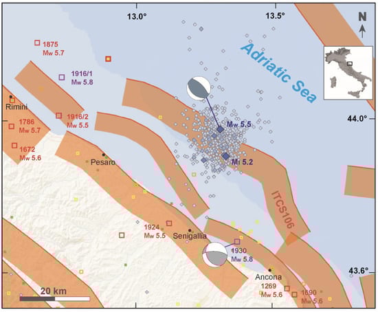
Figure 1.
Seismotectonic framework of the northern Marche coastal and offshore area. The seismic sequence from 9 November to 14 February 2023 is shown in light blue (http://terremoti.ingv.it/, accessed on 14 February 2023); historical and instrumental earthquakes from CPTI15 are shown with coloured squares (Rovida et al. [18]), earthquakes with are labelled (see Table 1); surface projection of Composite Seismogenic Sources from DISS 3.3.0 are shown with orange ribbons (https://diss.ingv.it, accessed on 14 February 2023; DISS_Working_Group [12]). Focal mechanisms of the 9 November 2022 earthquake and the 30 October 1930 event are from TDMT (http://webservices.ingv.it/webservices/ingv_ws_map/data/tdmt/19591/111604601_154_tdmt_reviewer_solution.pdf, accessed on 14 February 2023), and Vannoli et al. [19]), respectively.
The occurrence of historical and instrumental earthquakes (e.g., 1672, 1690, 1786, 1875, 1916, 1924, 1930, all with ; Table 1; Figure 1) suggests that the thrust faults are also seismogenic. The earthquakes in the area have often generated a tsunami; subsequently, their causative faults have been able to produce significant vertical displacement of the ground surface or sea floor, and are very close to the coast or offshore (Table 1; Vannoli et al. [19]).

Table 1.
Historical and instrumental earthquakes with of the study area (Figure 1; CPTI15; Rovida et al. [18]; CFTI5Med; Guidoboni et al. [21]), and tsunami with their intensity (EMTC; Maramai et al. [22]). T: true; SA: Intensity Sieberg–Ambraseys scale; PI: Intensity Papadopoulos and Imamura scale; * unspecified day; ** the earthquake triggered a large landslide that fell into the sea on the eastern side of Monte Conero (CFTI5Med [21]); *** some historical sources describe the occurrence of a second large earthquake one hour after the first event (CFTI5Med [21]); **** EMS-98 scale; Tertulliani et al. [2].
A relevant aspect of seismic activity in the study area, as in the rest of Italy (e.g., Vannoli et al. [20]), is the occurrence of seismic sequences with more than one main shock of similar magnitude (Table 1). These sequences can be distinguished from typical aftershock sequences because the difference between the largest and second-largest magnitudes is relatively small and does not follow the so-called “Bath Law” (see Console et al. [7]).
A seismic sequence with two events of similar magnitude also began on 9 November 2022. As a matter of fact, at 06:07:25 UTC a earthquake struck the northern Marche offshore area, and only one minute later, a earthquake struck about 7 km to the south (http://terremoti.ingv.it, accessed on 14 February 2023; Figure 1; Table 1). According to the hypocentral location of these two mainshocks, the ITCS106 fault system is retained the causative source of the sequence. More than 900 aftershocks occurred offshore Pesaro and Senigallia from 9 November 2022 to 14 February 2023 (Figure 1).
The occurrence of this sequence demonstrates that the buried offshore thrust front, included in the Database of Individual Seismogenic Sources since 2013 despite the absence of historical and recent seismicity (DISS_Working_Group [12]), is active and seismogenic. Specifically, the ITCS106 Pesaro mare-Cornelia source straddles the Adriatic sea just north of the city of Ancona, and it is part of the Umbro-Marche Apennines outer offshore thrust. ITCS106 is a blind fault system believed capable of infrequent moderate-size earthquakes. Its slip rate, a main ingredient of the earthquake simulators and seismic hazard model, is in the range of 0.20–0.52 mm/yr (DISS_Working_Group [12] and reference therein). Therefore, ITCS106 can produce only subtle displacement of the Adriatic sea floor, even when it is accumulated over several seismic cycles.
3. Earthquake Simulation Method
Our simulator code’s algorithm was originally introduced by Console et al. [8], and subsequently modified in different versions with the inclusion of new features, as described by Console et al. [7,9]. The present study employs the following fundamental principles of the simulator algorithm:
- The simulation of seismic sources involves the use of planar quadrilateral fault segments with specific spatial position, shape, and size. To accurately represent the various seismic events that may occur, each fault segment is discretized by square cells with sizes determined by the minimum magnitude of events expected in the output simulated catalogue.
- At the start of the simulation, stress values are randomly assigned to each cell from a specified stress range. This randomization is essential to ensure that the simulation represents the natural variation in stress levels that exists in real-life seismic events.
- Every fault segment is subjected to constant and uniform tectonic stress loading. This loading is based on geologically or geodetically inferred slip rate, providing the simulation with a more accurate representation of the tectonic stresses that occur in real seismic events.
- The simulation involves the nucleation of a new event in a cell when its stress exceeds a given threshold strength. This threshold strength is essential to accurately model the conditions that trigger seismic events in reality.
- Whenever a cell ruptures, a co-seismic stress-drop of 3.3 MPa is assigned to it. This stress-drop is a crucial aspect of the simulation as it represents the stress released by the rupturing cell, which is a significant factor in the generation of seismic events.
- Following the rupture of a cell, the co-seismic Coulomb stress is transferred from the rupturing cell to all other neighbouring cells. This transfer occurs based on the theory of elasticity, taking into account the strike, dip, and rake of each cell.
- The rupture expands to neighbouring cells based on heuristic rules that simulate a weakening mechanism. These rules are based on the behaviour of real-life seismic events and are essential to accurately represent the spread of a seismic event.
- If the positive Coulomb stress transferred from neighbouring cells causes a cell’s status to exceed the threshold strength, it is allowed to rupture more than once in the same earthquake. This is an important aspect of the simulation as it allows for the accurate representation of aftershocks and the complex nature of seismic events.
- The simulation algorithm allows ruptures to jump from one fault segment to another (even if they belong to two different faults) if their distance is shorter than a limit assigned by the user. This feature is essential to accurately represent the interaction of seismic events and the way in which they can trigger each other.
- The rupture stops when the stress of no neighbouring cell exceeds the computed strength threshold. This feature is important to ensure that the simulation accurately represents the natural behaviour of seismic events, which eventually reach a point where no further energy can be released.
The reason for choosing a trapezoidal shape for the seismic sources is to achieve a more precise representation of curved seismic structures. For instance, this helps to reduce gaps that may exist between adjacent rectangular segments when they do not have the same strike. It should be noted that using fault segments of rectangular or trapezoidal shapes to model seismic sources constitutes a simplification of the algorithm adopted in our physics-based simulation code. It is not a constraint that implies a rupture stops at the edges of every segment.
The simulator algorithm has two free parameters that control how a rupture nucleates, propagates, and stops. The first of these parameters is “Strength Reduction” (S-R), which reduces the strength at the edges of growing ruptures through a sort of weakening mechanism. Increasing this parameter favors the growth of ruptures and, consequently, it has the effect of decreasing the b-value of the frequency-magnitude distribution. The second parameter is “Aspect Ratio” (A-R), which is introduced to limit the effect of the S-R parameter when a rupture grows beyond certain specified limits. This parameter assumes a significant role in the frequency-magnitude distribution in the range of large magnitudes, as shown in Figure 5 of Console et al. [8].
It is important to note that neither of the free parameters mentioned above influences the long-term annual seismic moment rate of the simulated seismicity, which depends only on the slip rate assigned to the simulator within the kinematic fault model. In this study, we analysed the simulations computed by Console et al. [6] with the free parameters S-R = 0.2 and A-R = 5, obtaining a synthetic catalogue characterised by a b-value of the Gutenberg–Richter distribution equal to 0.95 and a realistic production of multiple events.
4. Simulation of the Seismicity in the Adriatic Thrust Fault Systems
In the application of the simulator, the quadrilateral segments representing the ITCS106 fault system were discretized in cells of 1.0 km × 1.0 km. As to the slip rate, we adopted the value of 0.5 mm/year corresponding to the top value of the range reported by the DISS 3.3.0 database for this source. We found in previous applications of the simulator to central and northern Apennines Console et al. [6,7,9] that the largest slip rate is the one that better matches the annual rate of seismic moment obtained from instrumental observations.
We chose for the synthetic catalogues a minimum magnitude of 4.2, which is produced approximately by the rupture of two cells. Magnitude 4.3 is not present in the output catalogue because the rupture of three cells produces an event of magnitude 4.4. The duration of the synthetic catalogue was 100,000 years. A warm up period, the events of which are not included in the output catalogue, is necessary to bring the system in a stable situation. This period should be longer than a few inter-event times of the strongest magnitude. In this regard, we chose a warm up period of 10,000 years.
In this study, still taking into account the interactions from other sources, we limited our analysis to the above-mentioned ITCS106 source in the Adriatic sea, where the November–February 2023 earthquake sequence took place. At first, for this source we considered the magnitude–frequency distribution. Figure 2 shows a clear deviation of the magnitude–frequency distribution obtained by our simulation algorithm from a plain linear Gutenberg–Richter distribution. In fact, the incremental magnitude–frequency distribution shows a fairly linear trend with a b-value slightly greater than 1.0 up to magnitude 5.5, but it exhibits a sharp “bump” around magnitude 6.5, This value could be defined as “characteristic” for the considered fault system, and is related to its dimensions. It can also be noted that the cumulative magnitude distribution of the synthetic catalogue is characterised by a very small b-value (i.e., a b-value slightly larger than 0) in the magnitude range 5.5 < M < 6.5.
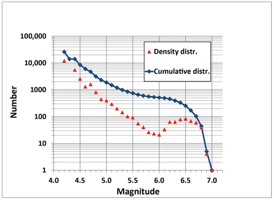
Figure 2.
Incremental magnitude–frequency distribution of the earthquakes in the synthetic catalogue obtained from the simulation algorithm (triangles) and the corresponding cumulative distribution (diamonds).
Our results are consistent with those of other studies where the magnitude–frequency distribution is analysed on individual faults, ignoring the contribution of smaller surrounding sources. For instance, Parsons et al. [10], by means of various statistical methods, demonstrated strongly characteristic magnitude–frequency distributions on the San Andreas fault, with a nearly flat cumulative distribution in the 6.5–7.5 magnitude range, and higher rates of large earthquakes than what would be expected from a Gutenberg–Richter distribution. The difference of approximately 1 magnitude unit between the results obtained for the ITCS106 fault system (about 70 km long) and the Saint Andreas fault (several hundreds of km long) is easily justified by their different dimensions.
We focused our attention on the inter-event times between events for the simulated catalogue of 100,000 yrs for earthquakes of magnitude equal to or larger than magnitudes 5.5, 6.0 and 6.5, respectively. The smallest size of 5.5 was the magnitude threshold adopted for the pivot earthquake of a multiple event by Console et al. [6]. According to popular scaling relationships (Leonard [23]) magnitude 6.5 is expected for the largest size of an earthquake that may rupture the entire area of the ITCS106 fault system. Table 2 reports the results of the statistical analysis carried out on the simulated catalogue, and Figure 3 shows the number of inter-event times in bins of 250 yrs.
Table 2.
Results of the statistical analysis of the simulated 100,000 yrs earthquake catalogue for the DISS composite source labelled ITCS106 for three different magnitudes thresholds. = recurrence time, = standard deviation, = coefficient of variation.
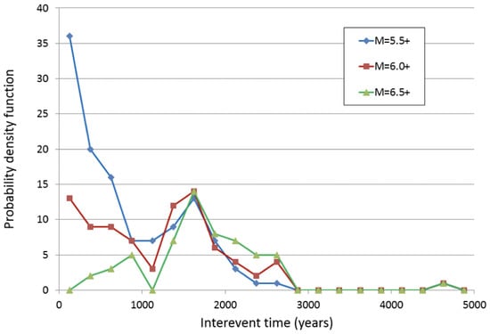
Figure 3.
Density distributions of the number of inter-event times in bins of 250 yrs. The first bin corresponds to the range of 0–250 yrs and so on.
The plot of Figure 3 shows a bi-modal distribution of inter-event times with a local minimum at 1000–1250 yrs. Smaller inter-event times are pertinent to clustering (with particular regard to small magnitude earthquakes), while the maximum at 1500–1750 yrs denotes quasi-periodicity (typical of larger magnitude earthquakes).
As expected, the number of events decreases and the average inter-event time increases when the magnitude threshold is increased (Table 2). However, the standard deviation maintains a value close to 700 yrs. In this way, the coefficient of variation (), which is defined by the ratio between and , decreases from 0.90 for to 0.40 for . It is well known that is equal to 1.0 for a sequence of events following a memoryless Poisson distribution and is equal to 0 for a perfectly periodical sequence. Thus, the earthquake sequence of our simulated catalogue behaves more and more as a quasi-periodical process when, increasing the threshold magnitude of the analysis, the ruptured areas of the considered earthquakes approach the size of whole seismic structure.
Shortest inter-event times (smaller than 1000 yrs) are typical of small magnitude earthquakes (Table 2, and Figure 3), while the opposite situation happens for the inter-event times larger than 2000 years (Figure 3). An exceptionally long inter-event time of 4625 yrs is estimated between two earthquakes of magnitude larger than 6.5 (Figure 3).
The simulations analysed in this study were obtained adopting the largest slip rates reported for the earthquake source in the DISS database. If we adopted smaller slip rates, the time scale of our inter-event times would become inversely longer.
The synthetic 100,000-year catalogue highlights a spatiotemporal behaviour that can hardly be compared with analog features observed in reality, due to their brevity, but can be considered realistic in light of an earthquake cycle hypothesis.
Long-term patterns preceding and following a strong earthquake are shown in Figure 4. This figure is obtained by stacking the number of earthquakes before and after an earthquake within a distance of 20 km between their respective epicenters in bins of 5 years. Here, we can observe an increase in seismic activity starting a couple of centuries before a strong earthquake, and a sharp increase in occurrence rate in the first 5 years after that event. The latter feature is clearly related to aftershock sequences following strong events. After this aftershock phase, the plot shows a long-lasting quiescence with some modest fluctuations. This long-term pattern highlights the existence of a preparatory phase before every strong earthquake. Presumably, during this preparatory phase, stress accumulation causes an increase in the rate of moderate-magnitude events. This hypothesis is supported by a detailed study of the time history of the average stress and its standard deviation during several seismic cycles in the Corinth (Greece) and Nankai (Japan) fault systems (Console and Carluccio [24], Console et al. [25]).
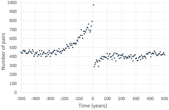
Figure 4.
Stacked number of earthquakes that preceded and followed an earthquake within an epicentral distance of 20 km in the 100,000 years simulated catalogue.
5. Conclusions
A seismic sequence initiated by a pair of mainshocks of magnitude 5.5 and 5.2 took place in the Northern Adriatic sea on 9 November 2022 at 06:07 UTC. The two mainshocks were separated by only one minute in time and about 10 km in space (Figure 1). The sequence is believed to be generated by the ITCS106 seismogenic source of the DISS database, belonging to the series of NW–SE trending, NE verging folds forming the easternmost edge of the Apennines thrust front (Figure 1).
Due to its low slip rate, estimated between 0.2 and 0.5 mm/yr in the DISS database, the ITCS106 source is characterised by moderate seismic activity, so as no earthquakes with were reported in the Parametric Catalogue of Italian Earthquakes from 1000 to 2020, before the two mainshocks of 9 November 2022. The occurrence of these earthquakes supports the hypothesis that even sources of low slip rate identified and characterised in the DISS database, for which little or no historical information is reported in the historical catalogues, may have seismic potential to be considered relevant in the context of seismic hazard assessment.
To quantify this hypothesis, we performed a statistical analysis of the results obtained by a previously developed simulator algorithm (Console et al. [6]) for the ITCS106 fault system. The results of our simulation consist of a catalogue of 100,000 yrs duration, containing 121, 84 and 57 earthquakes of magnitude equal to or exceeding a magnitude of 5.5, 6.0 and 6.5, respectively. The statistical analysis of the synthetic catalogue, shortly reported in Table 2, puts in evidence that the earthquakes belonging to the lowest magnitude class have an average inter-event time of yrs, while those belonging to the highest magnitude class have an average inter-event time of yrs. Consequently, the simulated catalogue exhibits a nearly memoryless Poissonian behaviour for moderate-magnitude earthquakes (whose coefficient of variation is 0.9), and a time-dependent quasi-periodic behaviour for large-magnitude earthquakes (whose coefficient of variation is 0.4). The statistical features obtained by the application of our earthquake simulator appear consistent with the hypothesis of the earthquake cycle. In this respect, our work may be relevant for possible applications related to the recent method of earthquake nowcasting (Rundle et al. [26,27], Varotsos et al. [28], Christopoulos et al. [29]), in which interoccurrence natural time between strong earthquakes is used for the estimation of the current stage of the earthquake cycle (see e.g., Varotsos et al. [30,31]).
Another significant aspect of our results is the acceleration of seismic activity before strong earthquakes lasting a couple of centuries in the ITCS106 seismic source. We conclude by suggesting that statistical parameters derived by physics-based earthquake simulators, even recognizing the limitations connected with the extreme simplicity of simulators, could be of support for the comprehension and modelling of seismic processes in situations where there is a lack of suitable observations for earthquake hazard assessment.
Author Contributions
Conceptualization, R.C. (Rodolfo Console), P.V. and R.C. (Roberto Carluccio); Validation, R.C. (Rodolfo Console) and P.V.; Data curation, R.C. (Roberto Carluccio); Writing—review & editing, R.C. (Rodolfo Console), Paola Vannoli and R.C. (Roberto Carluccio). All authors have read and agreed to the published version of the manuscript.
Funding
This research received no external funding.
Data Availability Statement
The Italian Parametric Earthquake Catalogue (CPTI15) can be found at https://emidius.mi.ingv.it/CPTI15-DBMI15/ (accessed on 14 February 2023), the Database of Individual Seismogenic Sources (DISS) can be found at http://diss.ingv.it (accessed on 14 February 2023).
Acknowledgments
The authors are grateful to Jörg Renner, Eleftheria Papadimitriou and anonymous reviewers for their careful reading of the manuscript and useful suggestions.
Conflicts of Interest
The authors declare no conflict of interest.
Abbreviations
The following abbreviations are used in this manuscript:
| CPTI | The Italian Parametric Earthquake Catalogue |
| DISS | The Database of Individual Seismogenic Sources |
| EMTC | Euro-Mediterranean Tsunami Catalogue |
| CFTI | Strong Italian Earthquakes Catalogue |
References
- ISIDe_Working_Group. Italian Seismological Instrumental and Parametric Database (ISIDe); Istituto Nazionale di Geofisica e Vulcanologia: Roma, Italy, 2007. [Google Scholar] [CrossRef]
- Tertulliani, A.; Antonucci, A.; Berardi, M.; Borghi, A.; Brunelli, G.; Caracciolo, C.H.; Castellano, C.; D’Amico, V.; Del Mese, S.; Ercolani, E.; et al. Gruppo Operativo Quest Rilievo Macrosismico MW 5.5 Costa Marchigiana del 9/11/2022 Rapporto Finale del 15/11/2022. Available online: https://www.earth-prints.org/handle/2122/15794 (accessed on 23 December 2022).
- Schultz, K.W.; Sachs, M.K.; Yoder, M.R.; Rundle, J.B.; Turcotte, D.L.; Heien, E.M.; Donnellan, A. Virtual quake: Statistics, co-seismic deformations and gravity changes for driven earthquake fault systems. In Proceedings of the International Symposium on Geodesy for Earthquake and Natural Hazards (GENAH), Matsushima, Japan, 22–26 July 2014; Springer: Cham, Switzerland, 2017; pp. 29–37. [Google Scholar]
- Christophersen, A.; Rhoades, D.; Colella, H. Precursory seismicity in regions of low strain rate: Insights from a physics-based earthquake simulator. Geophys. J. Int. 2017, 209, 1513–1525. [Google Scholar] [CrossRef]
- Field, E.H. How physics-based earthquake simulators might help improve earthquake forecasts. Seismol. Res. Lett. 2019, 90, 467–472. [Google Scholar] [CrossRef]
- Console, R.; Vannoli, P.; Carluccio, R. Physics-Based Simulation of Sequences with Foreshocks, Aftershocks and Multiple Main Shocks in Italy. Appl. Sci. 2022, 12, 2062. [Google Scholar] [CrossRef]
- Console, R.; Murru, M.; Vannoli, P.; Carluccio, R.; Taroni, M.; Falcone, G. Physics-based simulation of sequences with multiple main shocks in Central Italy. Geophys. J. Int. 2020, 223, 526–542. [Google Scholar] [CrossRef]
- Console, R.; Carluccio, R.; Papadimitriou, E.; Karakostas, V. Synthetic earthquake catalogs simulating seismic activity in the Corinth Gulf, Greece, fault system. J. Geophys. Res. Solid Earth 2015, 120, 326–343. [Google Scholar] [CrossRef]
- Console, R.; Vannoli, P.; Carluccio, R. The seismicity of the Central Apennines (Italy) studied by means of a physics-based earthquake simulator. Geophys. J. Int. 2018, 212, 916–929. [Google Scholar] [CrossRef]
- Parsons, T.; Geist, E.L.; Console, R.; Carluccio, R. Characteristic earthquake magnitude frequency distributions on faults calculated from consensus data in California. J. Geophys. Res. Solid Earth 2018, 123, 10–761. [Google Scholar] [CrossRef]
- Gulia, L.; Wiemer, S. Real-time discrimination of earthquake foreshocks and aftershocks. Nature 2019, 574, 193–199. [Google Scholar] [CrossRef]
- DISS_Working_Group. Database of Individual Seismogenic Sources (DISS), Version 3.3.0: A Compilation of Potential Sources for Earthquakes Larger Than M 5.5 in Italy and Surrounding Areas; Istituto Nazionale di Geofisica e Vulcanologia: Roma, Italy, 2021; Available online: http://diss.rm.ingv.it/diss/ (accessed on 14 February 2023). [CrossRef]
- Vannoli, P.; Basili, R.; Valensise, G. New geomorphic evidence for anticlinal growth driven by blind-thrust faulting along the northern Marche coastal belt (central Italy). J. Seismol. 2004, 8, 297–312. [Google Scholar] [CrossRef]
- Fantoni, R.; Franciosi, R. Tectono-sedimentary setting of the Po Plain and Adriatic foreland. Rend. Lincei 2010, 21, 197–209. [Google Scholar] [CrossRef]
- Kastelic, V.; Vannoli, P.; Burrato, P.; Fracassi, U.; Tiberti, M.M.; Valensise, G. Seismogenic sources in the Adriatic Domain. Mar. Pet. Geol. 2013, 42, 191–213. [Google Scholar] [CrossRef]
- Elter, P.; Giglia, G.; Tongiorgi, M.; Trevisan, L. Tensional and Compressional Areas in the Recent (Tortonian to Present) Evolution of the Northern Apennines. Bollettino di Geofisica Teorica ed Applicata 1975, 17, 3–18. [Google Scholar]
- Maesano, F.E.; Toscani, G.; Burrato, P.; Mirabella, F.; D’Ambrogi, C.; Basili, R. Deriving thrust fault slip rates from geological modeling: Examples from the Marche coastal and offshore contraction belt, Northern Apennines, Italy. Mar. Pet. Geol. 2013, 42, 122–134. [Google Scholar] [CrossRef]
- Rovida, A.N.; Locati, M.; Camassi, R.D.; Lolli, B.; Gasperini, P.; Antonucci, A. Catalogo Parametrico dei Terremoti Italiani CPTI15, Versione 4.0; Istituto Nazionale di Geofisica e Vulcanologia (INGV): Roma, Italy, 2022. [Google Scholar] [CrossRef]
- Vannoli, P.; Vannucci, G.; Bernardi, F.; Palombo, B.; Ferrari, G. The source of the 30 October 1930 M w 5.8 Senigallia (Central Italy) earthquake: A convergent solution from instrumental, macroseismic, and geological data. Bull. Seismol. Soc. Am. 2015, 105, 1548–1561. [Google Scholar] [CrossRef]
- Vannoli, P.; Bernardi, F.; Palombo, B.; Vannucci, G.; Console, R.; Ferrari, G. New constraints shed light on strike-slip faulting beneath the southern Apennines (Italy): The 21 August 1962 Irpinia multiple earthquake. Tectonophysics 2016, 691, 375–384. [Google Scholar] [CrossRef]
- Guidoboni, E.; Ferrari, G.; Mariotti, D.; Comastri, A.; Tarabusi, G.; Sgattoni, G.; Valensise, G. CFTI5Med, Catalogo dei Forti Terremoti in Italia (461 aC-1997) e nell’area Mediterranea (760 aC-1500); Istituto Nazionale di Geofisica e Vulcanologia (INGV): Rome, Italy, 2018. [Google Scholar] [CrossRef]
- Maramai, A.; Graziani, L.; Brizuela, B. Euro-Mediterranean Tsunami Catalogue (EMTC), Version 2.0; Istituto Nazionale di Geofisica e Vulcanologia (INGV): Rome, Italy, 2019. [Google Scholar] [CrossRef]
- Leonard, M. Self-consistent earthquake fault-scaling relations: Update and extension to stable continental strike-slip faults. Bull. Seismol. Soc. Am. 2014, 104, 2953–2965. [Google Scholar] [CrossRef]
- Console, R.; Carluccio, R. Earthquake Simulators Development and Application. In Statistical Methods and Modeling of Seismogenesis; Wiley: New York, NY, USA, 2021; p. 27. [Google Scholar]
- Console, R.; Carluccio, R.; Murru, M.; Papadimitriou, E.; Karakostas, V. Physics-Based Simulation of Spatiotemporal Patterns of Earthquakes in the Corinth Gulf, Greece, Fault System. Bull. Seismol. Soc. Am. 2022, 112, 98–117. [Google Scholar] [CrossRef]
- Rundle, J.B.; Turcotte, D.; Donnellan, A.; Grant Ludwig, L.; Luginbuhl, M.; Gong, G. Nowcasting earthquakes. Earth Space Sci. 2016, 3, 480–486. [Google Scholar] [CrossRef]
- Rundle, J.B.; Stein, S.; Donnellan, A.; Turcotte, D.L.; Klein, W.; Saylor, C. The complex dynamics of earthquake fault systems: New approaches to forecasting and nowcasting of earthquakes. Rep. Prog. Phys. 2021, 84, 076801. [Google Scholar] [CrossRef] [PubMed]
- Varotsos, P.K.; Perez-Oregon, J.; Skordas, E.S.; Sarlis, N.V. Estimating the epicenter of an impending strong earthquake by combining the seismicity order parameter variability analysis with earthquake networks and nowcasting: Application in the Eastern Mediterranean. Appl. Sci. 2021, 11, 10093. [Google Scholar] [CrossRef]
- Christopoulos, S.R.G.; Varotsos, P.K.; Perez-Oregon, J.; Papadopoulou, K.A.; Skordas, E.S.; Sarlis, N.V. Natural Time Analysis of Global Seismicity. Appl. Sci. 2022, 12, 7496. [Google Scholar] [CrossRef]
- Varotsos, P.; Sarlis, N.; Skordas, E.; Uyeda, S.; Kamogawa, M. Natural-time analysis of critical phenomena: The case of seismicity. Europhys. Lett. 2010, 92, 29002. [Google Scholar] [CrossRef]
- Varotsos, P.; Sarlis, N.V.; Skordas, E.S.; Uyeda, S.; Kamogawa, M. Natural time analysis of critical phenomena. Proc. Natl. Acad. Sci. USA 2011, 108, 11361–11364. [Google Scholar] [CrossRef] [PubMed]


Disclaimer/Publisher’s Note: The statements, opinions and data contained in all publications are solely those of the individual author(s) and contributor(s) and not of MDPI and/or the editor(s). MDPI and/or the editor(s) disclaim responsibility for any injury to people or property resulting from any ideas, methods, instructions or products referred to in the content. |
© 2023 by the authors. Licensee MDPI, Basel, Switzerland. This article is an open access article distributed under the terms and conditions of the Creative Commons Attribution (CC BY) license (https://creativecommons.org/licenses/by/4.0/).