A New Generalized Logarithmic–X Family of Distributions with Biomedical Data Analysis

Abstract

In this article, an attempt is made to propose a novel method of lifetime distributions with maximum flexibility using a popular T–X approach together with an exponential distribution, which is known as the New Generalized Logarithmic-X Family (NGLog–X for short) of distributions. Additionally, the generalized form of the Weibull distribution was derived by using the NGLog–X family, known as the New Generalized Logarithmic Weibull (NGLog–Weib) distribution. For the proposed method, some statistical properties, including the moments, moment generating function (MGF), residual and reverse residual life, identifiability, order statistics, and quantile functions, were derived. The estimation of the model parameters was derived by using the well-known method of maximum likelihood estimation (MLE). A comprehensive Monte Carlo simulation study (MCSS) was carried out to evaluate the performance of these estimators by computing the biases and mean square errors. Finally, the NGLog–Weib distribution was implemented on four real biomedical datasets and compared with some other distributions, such as the Alpha Power Transformed Weibull distribution, Marshal Olkin Weibull distribution, New Exponent Power Weibull distribution, Flexible Reduced Logarithmic Weibull distribution, and Kumaraswamy Weibull distribution. The analysis results demonstrate that the new proposed model performs as a better fit than the other competitive distributions.

1. Introduction

To model and analyse lifetime data, probability distributions are essential tools, particularly in the area of biomedical science; see Liu et al. [1]. Various probability distributions have been suggested for modelling lifetime phenomena; for example, the Exponential (Expo), Rayleigh (Ray), and Weibull (Weib) distributions. However, the performance of these aforementioned classical distributions is affected when the phenomena are complex. For illustration, the commonly used Expo distribution performs well for modelling lifetime phenomena based on a constant hazard rate function (HRF), whereas the Ray distribution has the ability to model lifetime phenomena having only an increasing HRF. The Weib distribution is known for its performance, as it has the characteristics of both the Expo and Ray distributions. The Weib distribution can model the phenomena having a monotone (increasing, decreasing, and constant) HRF (see Almalki and Yuan [2], and Liao et al. [3]). However, when the phenomena follow non-monotonic (unimodal, modified unimodal, and bathtub-shaped) HRFs, the Weib distribution may not be a good option. In medical cases, e.g., breast cancer, neck cancer, and bladder cancer, the HRF of the phenomena is shown to have a uni-modal or modified uni-modal shape. The HRF for breast cancer, bladder cancer, and neck cancer has been identified as a uni-modal shape after surgical removal. The cancer recurrence HRF begins to increase in the early stage and gradually decreases after a definite period of time when removed by surgery (Demicheli et al. [4]). Another example of a uni-modal failure rate is infection with some new viruses, where the initial phase increases and then decreases; see, for example, (Liu et al. [1]).

In the recent past, researchers have contributed toward developing new families of continuous probability distributions that are flexible in nature. These flexible distributions are derived by incorporating some additional parameters into the baseline distributions. Here, we refer to some of the newly proposed families of lifetime distributions, including: the Marshall–Olkin Weibull–Generated (MO–Weib–G) family of probability distributions proposed by Klakattawi et al. [5], the Shifted Exponential–G (SExpo–G) family of distributions proposed by Eghwerido et al. [6], the Generalization of Gull Alpha Power (GGAP) family of probability distributions proposed by Kilai et al. [7], the New Flexible Logarithmic–X (NFLog–X) family of probability distributions proposed by Alkhairy et al. [8], the Arcsine–X family of probability distributions proposed by Tung et al. [9], the Truncated family of distributions proposed by Alzaatreh et al. [10], the Transmuted Alpha Power–G (TAP–G) family of Eghwerido et al. [11], the Fréchet Topp Leone–G (FTL–G) family of Reyad et al. [12], the New Extended-Family (NEx-F) of distributions proposed by Zichuan et al. [13], a New Lifetime Exponential–X (NLE–X) family proposed by Huo et al. [14], a New Modified Exponent Power Alpha (NMEPA) family of distributions proposed by Shah et al. [15], and a generalized Alpha Exponent Power (GAEP) Family of distributions proposed by Hussain et al. [16]. For more reading about probability distributions, see Chen et al. [17], Xu et al. [18], Zhang et al. [19], Luo et al. [20], and Zhuang et al. [21].

Zhao et al. [22] have introduced a new method of lifetime distributions by incorporating an additional parameter using the T–X family method (Alzaatreh et al. [23]). The CDF (cumulative distribution function) is given by

$$G\left(x;\delta ,\Theta \right)=1-{\left(\frac{1-F\left(x;\Theta \right)}{1-(1-\delta )F\left(x;\Theta \right)}\right)}^{\delta }\hspace{1em}x\in ℝ$$

(1)

where $\delta \in {ℝ}^{+}$ is the shape parameter, and $F\left(x;\Theta \right)$ is the CDF of any baseline distribution.

Wang et al. [24] have suggested a new logarithmic family of lifetime distributions, and its CDF is

$$G\left(x;\delta ,\theta ,\Theta \right)=\frac{\log \left[e^{\delta }-\left(1-F{\left(x;\Theta \right)}^{\theta }\right)\left(e^{\delta }-1\right)\right]}{\delta }\hspace{1em}x\in ℝ$$

(2)

where $\delta \in {ℝ}^{+}$ and $\theta \in {ℝ}^{+}$ are the additional parameters, and $F\left(x;\Theta \right)$ is the CDF of any baseline or classical distribution.

Likewise, another approach has been recommended for the lifetime phenomena modelling named the Log–U (Logarithmic–U) of distributions by Zhao et al. [25]. The CDF of the Log–U family is

$$G\left(x;\theta ,\alpha ,\Theta \right)=1-{\left(1-\frac{\alpha F\left(x;\Theta \right)}{\alpha -\left[\log F\left(x;\Theta \right)\right]}\right)}^{\theta }\hspace{1em}x\in ℝ$$

(3)

where $\alpha \in {ℝ}^{+}$ and $\theta \in {ℝ}^{+}$ are the additional parameters, and $F\left(x;\Theta \right)$ is the CDF of any baseline or classical distribution.

In this paper, we carry this approach of distribution theory and propose a new family of probability distributions by implementing the T–X family approach (Alzaatreh et al. [23]). The proposed family of distributions gives an appropriate fit for biomedical datasets. Additionally, this study empirically shows that the new extension of the Weib distribution offers an efficient fit to the considered datasets in comparison with well-known distributions (see Section 6).

The work carried out in this paper is outlined and organized in the following sections: In Section 2, the new method of lifetime distributions is derived. In Section 3, a three-parameter special subcase of the proposed class named a New Generalized Logarithmic Weibull (NGLog–Weib) distribution is derived, and the shape of the CDF, PDF (probability density function), and HF (hazard function) are also discussed in the same section. In Section 4, some mathematical and statistical properties of the proposed approach are derived. In Section 5, the estimation methods for estimating the modal parameters are used, as well as in the same section, a brief MCSS is also conducted to assess the behaviour of these estimates. The implementations of the novel-introduced methods on four biomedical datasets are discussed in Section 6.

2. The NGLog–X Family

Let $r\left(t\right)$ be the PDF of a RV (random variable), say $T$, where $T\in \left[{\pi }_1,{\pi }_2\right]$ for $-\infty \le {\pi }_1<{\pi }_2<\infty$, and let suppose that $K\left[F(x;\Theta )\right]$ be a function of $F(x;\Theta )$ CDF of a RV, say $X$, satisfying the conditions given bellow:

i.

$K\left[F(x;\Theta )\right]\in \left({\pi }_1,{\pi }_2\right)$;

ii.

$K\left[F(x;\Theta )\right]$ is monotonically increasing and differentiable; and

iii.

$K\left[F(x;\Theta )\right]\to {\pi }_1$ as $x\to -\infty$ and $K\left[F(x;\Theta )\right]\to {\pi }_2$ as $x\to \infty$.

According to (Alzaatreh et al. [23]), the CDF $G\left(x\right)$ of the T–X family is defined by

$$G\left(x\right)={\displaystyle {\int }_{{\pi }_1}^{K[F\left(x;\Theta \right)]}r\left(t\right)}dt,\hspace{1em}x\in ℝ.$$

(4)

The $g\left(x\right)$ PDF corresponding to (4) is given by

$$g\left(x\right)=\left\{\frac{d}{dx}K[F\left(x;\Theta \right)]\right\}r\left\{K[F\left(x;\Theta \right)]\right\},\hspace{1em}x\in ℝ.$$

Using the T–X idea, several novel classes of distributions have been proposed in the literature. Table 1 lists different $K\left[F(x;\Theta )\right]$ functions for special members of the T–X family.

Table 1. Different $K\left[F(x;\Theta )\right]$ functions for some members of the T–X family.

$K\left[F(x;\Theta )\right]$	Support of X	Member of T–X Family
$F(x;\Theta )$	$[0,1]$	Beta–G (Eugen et al. [26])
$-\log \left[F(x;\Theta )\right]$	$(0,\infty )$	Gamma–G type 1 (Zografos and Balakrishnan [27])
$-\log \left[1-F(x;\Theta )\right]$	$(0,\infty )$	Gamma–G type 2 (Ristic and Balakrishnan [28])
$\frac{F(x;\Theta )}{1-F(x;\Theta )}$	$(0,\infty )$	Gamma–G type 3 (Torabi and Montazeri [29])
$\log \left[-\log \left\{1-F(x;\Theta )\right\}\right]$	$(-\infty ,\infty )$	Logistic–X family (Tahir et al. [30])
$-\log \left(\frac{1-F(x;\Theta )}{e^{F(x;\Theta )}}\right)$	$(0,\infty )$	Weighted T–X family (Ahmad et al. [31])
$-\log \left[\frac{e^{(1-K(x,\Theta \left)\right)}-1}{e-(1-K(x,\Theta \left)\right)}\right]$	$(0,\infty )$	New Expo–X family (Shah et al. [32])
$-\log \left(\frac{e^{\delta }F\left(x;\Theta \right)}{{\left(e-\log F\left(x;\Theta \right)\right)}^{\delta }}\right)$	$(0,\infty )$	NGLog–X family (proposed)

Table 1. Different $K\left[F(x;\Theta )\right]$ functions for some members of the T–X family.

$K\left[F(x;\Theta )\right]$	Support of X	Member of T–X Family
$F(x;\Theta )$	$[0,1]$	Beta–G (Eugen et al. [26])
$-\log \left[F(x;\Theta )\right]$	$(0,\infty )$	Gamma–G type 1 (Zografos and Balakrishnan [27])
$-\log \left[1-F(x;\Theta )\right]$	$(0,\infty )$	Gamma–G type 2 (Ristic and Balakrishnan [28])
$\frac{F(x;\Theta )}{1-F(x;\Theta )}$	$(0,\infty )$	Gamma–G type 3 (Torabi and Montazeri [29])
$\log \left[-\log \left\{1-F(x;\Theta )\right\}\right]$	$(-\infty ,\infty )$	Logistic–X family (Tahir et al. [30])
$-\log \left(\frac{1-F(x;\Theta )}{e^{F(x;\Theta )}}\right)$	$(0,\infty )$	Weighted T–X family (Ahmad et al. [31])
$-\log \left[\frac{e^{(1-K(x,\Theta \left)\right)}-1}{e-(1-K(x,\Theta \left)\right)}\right]$	$(0,\infty )$	New Expo–X family (Shah et al. [32])
$-\log \left(\frac{e^{\delta }F\left(x;\Theta \right)}{{\left(e-\log F\left(x;\Theta \right)\right)}^{\delta }}\right)$	$(0,\infty )$	NGLog–X family (proposed)

Now, taking inspiration from Equation (4), we propose the novel-introduced family of distributions. Let $T~\exp (1)$, and then its CDF is given by

$$R\left(t\right)=1-e^{-t}, \hspace{1em}t\ge 0$$

(5)

The PDF corresponding to Equation (5) is

$$r\left(t\right)=e^{-t}, \hspace{1em}t>0$$

(6)

Setting $K[F\left(x;\Theta \right)]=-\log \left(\frac{e^{\delta }F\left(x;\Theta \right)}{{\left(e-\log F\left(x;\Theta \right)\right)}^{\delta }}\right)$ and $r\left(t\right)$ as Equation (6) in Equation (4), we obtain the $G\left(x;\delta ,\Theta \right)$ CDF of the New Generalized Logarithmic–X (NGLog–X) family of lifetime distributions, which is given by

$$G\left(x;\delta ,\Theta \right)=\frac{e^{\delta }F\left(x;\Theta \right)}{{\left(e-\log F\left(x;\Theta \right)\right)}^{\delta }}, \hspace{1em}\delta \in {ℝ}^{+},x\in ℝ$$

(7)

where $\delta \in {ℝ}^{+}$ is an extra shape parameter, $x\in ℝ$ and $F\left(x;\Theta \right)$ is the CDF of any baseline (or existing) probability distribution which may depend on a parameter vector $\Theta \in ℝ$.

The PDF $g\left(x;\delta ,\Theta \right)=\frac{d}{dx}G\left(x;\delta ,\Theta \right)$ corresponding to Equation (7) is given by

$$g\left(x;\delta ,\Theta \right)=\frac{f\left(x;\Theta \right)e^{\delta }\left\{1+\delta {\left(e-\log F\left(x;\Theta \right)\right)}^{-1}\right\}}{{\left(e-\log F\left(x;\Theta \right)\right)}^{\delta }},\delta \in {ℝ}^{+},x\in ℝ$$

(8)

where, $\frac{d}{dx}F\left(x;\Theta \right)=f\left(x;\Theta \right)$

Furthermore, for $\delta \in {ℝ}^{+}$ and $x\in ℝ$, the SF (survival function) $S\left(x;\delta ,\Theta \right)=1-G\left(x;\delta ,\Theta \right)$, HF (hazard function) $h\left(x;\delta ,\Theta \right)=\frac{g\left(x;\delta ,\Theta \right)}{1-G\left(x;\delta ,\Theta \right)}$, RHF (reverse hazard function) $\tau \left(x;\delta ,\Theta \right)=\frac{g\left(x;\delta ,\Theta \right)}{G\left(x;\delta ,\Theta \right)}$, and CHF (cumulative hazard function) $H\left(x;\delta ,\Theta \right)=-\log \left[1-G\left(x;\delta ,\Theta \right)\right]$ of the NGLog–X family are shown in Equations (9)–(12):

$$S\left(x;\delta ,\Theta \right)=1-\frac{e^{\delta }F\left(x;\Theta \right)}{{\left(e-\log F\left(x;\Theta \right)\right)}^{\delta }},$$

(9)

$$h\left(x;\delta ,\Theta \right)=\frac{f\left(x;\Theta \right)e^{\delta }\left\{1+\delta {\left(e-\log F\left(x;\Theta \right)\right)}^{-1}\right\}}{{\left(e-\log F\left(x;\Theta \right)\right)}^{\delta }-e^{\delta }F\left(x;\Theta \right)},$$

(10)

$$\tau \left(x;\delta ,\Theta \right)=\frac{f\left(x;\Theta \right)\left\{1+\delta {\left(e-\log F\left(x;\Theta \right)\right)}^{-1}\right\}}{F\left(x;\Theta \right)},$$

(11)

and

$$H\left(x;\delta ,\Theta \right)=-\log \left(1-\frac{e^{\delta }F\left(x;\Theta \right)}{{\left(e-\log F\left(x;\Theta \right)\right)}^{\delta }}\right)$$

(12)

3. NGLog–Weib Distribution

For a three-parameter special case of the NGLog–X family, let us consider the CDF,$F\left(x;\Theta \right)$, and PDF, $f\left(x;\Theta \right)$, of the traditional Weib distribution are $F\left(x;\Theta \right)=1-e^{-\beta x^{\alpha }}$ and $f\left(x;\Theta \right)=\beta \alpha x^{\alpha -1}{e}^{-\beta x^{\alpha }}$, respectively ($\beta \in {ℝ}^{+},\alpha \in {ℝ}^{+},$ and $x\in {ℝ}^{+}$), where $\Theta =\left(\beta ,\alpha \right)$.

Using $F\left(x;\Theta \right)=1-e^{-\beta x^{\alpha }}$ in Equation (7), we define the CDF $G\left(x;\delta ,\Theta \right)$ of the NGLog–Weib model. For $x\in {ℝ}^{+}$, the scale parameter, $\beta \in {ℝ}^{+}$, and shape parameters, $\delta \in {ℝ}^{+}$ and $\alpha \in {ℝ}^{+}$, the $G\left(x;\delta ,\Theta \right)$ CDF of the NGLog–Weib model is as follows,

$$G\left(x;\delta ,\Theta \right)=\frac{e^{\delta }\left(1-e^{-\beta x^{\alpha }}\right)}{{\left(e-\log \left(1-e^{-\beta x^{\alpha }}\right)\right)}^{\delta }},$$

(13)

$$S\left(x;\delta ,\Theta \right)=1-\frac{e^{\delta }\left(1-e^{-\beta x^{\alpha }}\right)}{{\left(e-\log \left(1-e^{-\beta x^{\alpha }}\right)\right)}^{\delta }},\hspace{1em}(\mathrm{Survival} \mathrm{Function})$$

(14)

Plots of the CDF, i.e., $G\left(x;\delta ,\Theta \right)$ and SF (survival function), i.e., $S\left(x;\delta ,\Theta \right)$ of the NGLog–Wei probability model, are given in Figure 1 for (i) $\delta =$ 2.0, $\beta =$ 6.0, $\alpha =$ 1.5 (in red), (ii) $\delta =$ 3.0, $\beta =$ 5.0, $\alpha =$ 2.3 (in green), (iii) $\delta =$ 4.0, $\beta =$ 3.0, $\alpha =$ 2.9 (in black), and (iv) $\alpha =$ 4.0, $\beta =$ 1.5, $\theta =$ 3.5 (in blue).

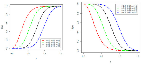
Figure 1. Plots of the $G\left(x;\delta ,\Theta \right)$ CDF (left) and the $S\left(x;\delta ,\Theta \right)$ SF (right) of the NGLog–Weib model.

Corresponding to $G\left(x;\delta ,\Theta \right)$ in Equation (13), the PDF,$g\left(x;\delta ,\Theta \right)$, is

$$g\left(x;\delta ,\Theta \right)=\frac{\alpha \beta x^{\alpha -1}{e}^{-\beta x^{\alpha }+\delta }\left\{1+\delta {\left(e-\log \left(1-e^{-\beta x^{\alpha }}\right)\right)}^{-1}\right\}}{{\left(e-\log \left(1-e^{-\beta x^{\alpha }}\right)\right)}^{\delta }}$$

(15)

For a graphical illustration, some possible behaviours of the PDF $g\left(x;\delta ,\Theta \right)$ of the NGLog–Weib distribution at different parameter values are sketched in Figure 2. The plots are sketched for (i) $\delta =$ 3.0, $\beta =$ 3.5, $\alpha =$ 0.3 (in red), (ii) $\delta =$ 3.0, $\beta =$ 5.0, $\alpha =$ 1.9 (in green), (iii) $\delta =$ 4.5, $\beta =$ 3.0, $\alpha =$ 2.9 (in black), and (iv) $\delta =$ 6.5, $\beta =$ 1.5, $\alpha =$ 3.3 (in blue). Figure 2 shows four different shapes of the PDF $g\left(x;\delta ,\Theta \right)$, including (i) decreasing or a reverse-J pattern (in red), (ii) right-skewed (in green), (iii) symmetrical (in black), and (iv) left-skewed (in blue).

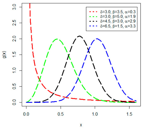
Figure 2. Plots of the $g\left(x;\delta ,\Theta \right)$ PDF of the NGLog–Weib model.

Furthermore, the hazard function $h\left(x;\delta ,\Theta \right)$, RHF (reverse hazard function) $\tau \left(x;\delta ,\Theta \right)$, and CHF (cumulative hazard function) $H\left(x;\delta ,\Theta \right)$ of the NGLog–Weib are given in Equations (16) to (18), respectively, by

$$h\left(x;\delta ,\Theta \right)=\frac{\alpha \beta x^{\alpha -1}{e}^{-\beta x^{\alpha }+\delta }\left\{1+\delta {\left(e-\log \left(1-e^{-\beta x^{\alpha }}\right)\right)}^{-1}\right\}}{{\left(e-\log \left(1-e^{-\beta x^{\alpha }}\right)\right)}^{\delta }-e^{\delta }\left(1-e^{-\beta x^{\alpha }}\right)},$$

(16)

$$\tau \left(x;\delta ,\Theta \right)=\frac{\beta \alpha x^{\alpha -1}{e}^{-\beta x^{\alpha }}\left\{1+\delta {\left(e-\log \left(1-e^{-\beta x^{\alpha }}\right)\right)}^{-1}\right\}}{\left(1-e^{-\beta x^{\alpha }}\right)},$$

(17)

$$H\left(x;\delta ,\Theta \right)=-\log \left(1-\frac{e^{\delta }\left(1-e^{-\beta x^{\alpha }}\right)}{{\left(e-\log \left(1-e^{-\beta x^{\alpha }}\right)\right)}^{\delta }}\right)$$

(18)

Furthermore, for the various values of the parameters, some possible behaviours of the HF $h\left(x;\delta ,\Theta \right)$ of the NGLog–Weib model are shown in Figure 3 for (i) $\delta =$ 10.7, $\beta =$ 2.6, $\alpha =$ 0.5 (in red), (ii) $\delta =$ 10.4, $\beta =$ 3.5, $\alpha =$ 0.5 (in green), (iii) $\delta =$ 0.5, $\beta =$ 0.2, $\alpha =$ 2.9 (in black), (iv) $\delta =$ 6.0, $\beta =$ 2.4, $\alpha =$ 0.3 (in blue), and (iv) $\delta =$ 0.5, $\beta =$ 0.8, $\alpha =$ 0.5 (in violet). From Figure 3, we can observe (or examine) that the NGLog–Wieb offers data modelling with increasing, decreasing, uni-model, and bathtub-shaped HFs, $h\left(x;\delta ,\Theta \right)$.

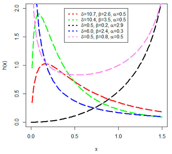
Figure 3. Plots of the $h\left(x;\delta ,\Theta \right)$ HF of the NGLog–Weib model.

4. Statistical Properties

This section presents some mathematical and statistical properties of the NGLog–X family of probability distributions.

4.1. Moments

We derived a computational representation of the general order moments corresponding to the proposed NGLog–X of distributions. If x is an RV from the NGLog–X family, then about the origin, the $r^{\mathrm{th}}$ moments are given by

$$E\left(x^r\right)={\displaystyle {\int }_{-\infty }^{\infty }{x}^{r}g(x;\delta ,\Theta )dx}$$

(19)

Putting the density of the proposed family in Equation (19), we obtain

$${\mu }^{\prime }={\displaystyle {\int }_{-\infty }^{\infty }{x}^r\frac{f\left(x;\Theta \right)e^{\delta }\left\{1+\delta {\left(e-\log F\left(x;\Theta \right)\right)}^{-1}\right\}}{{\left(e-\log F\left(x;\Theta \right)\right)}^{\delta }}dx}$$

$${\mu }^{\prime }={\displaystyle {\int }_{-\infty }^{\infty }{x}^{r}f\left(x;\Theta \right){\left(1-\frac{\log F\left(x;\Theta \right)}{e}\right)}^{-\delta }\left\{1+\delta e^{-1}{\left(1-\frac{\log F\left(x;\Theta \right)}{e}\right)}^{-1}\right\}dx}$$

(20)

Using the expansion ${\left(1-x\right)}^{-n}={\displaystyle \sum _{i=0}^{\infty }\left(\begin{array}{c}i+n-1\\ n-1\end{array}\right)} x^i$, where $x=\frac{\log F\left(x;\Theta \right)}{e}$, $n=\delta$, and $n=1$ in Equation (20), respectively, then we obtain

$${\mu }^{\prime }={\displaystyle \sum _{i=0}^{\infty }\left(\begin{array}{c}i+\delta -1\\ \delta -1\end{array}\right)e^{-i}{\Psi }_i+\delta {\displaystyle \sum _{i=0}^{\infty }{\displaystyle \sum _{j=0}^{\infty }\left(\begin{array}{c}i+\delta -1\\ \delta -1\end{array}\right)e^{-\left(i+j+1\right)}{\Psi }_{i,j,1}}}}$$

(21)

where

$${\Psi }_i={\displaystyle {\int }_{-\infty }^{\infty }{x}^{r}f\left(x;\Theta \right){\left(\log F\left(x;\Theta \right)\right)}^i}dx$$

and

$${\Psi }_{i,j,1}={\displaystyle {\int }_{-\infty }^{\infty }{x}^{r}f\left(x;\Theta \right){\left(\log F\left(x;\Theta \right)\right)}^{i+j}}dx$$

Similarly, using the PDF $g\left(x;\delta ,\Theta \right)$, a general explicit expression for the MGF (moments generating function) ${\mathrm{{\rm M}}}_X\left(t\right)$ of the NGLog–X is derived as

$${\mathrm{{\rm M}}}_X\left(t\right)={\displaystyle {\int }_{-\infty }^{\infty }{e}^{tx}g\left(x;\delta ,\Theta \right)dx}={\displaystyle \sum _{r=0}^{\infty }\frac{t^r}{r!}{\mu }^{\prime }}$$

(22)

By simplifying, we obtain the MGF

$${\mathrm{{\rm M}}}_X\left(t\right)={\displaystyle \sum _{i,r=0}^{\infty }\frac{t^r{e}^{-i}}{r!}}{\Psi }_i+\delta {\displaystyle \sum _{i,j,r=0}^{\infty }\frac{t^r{e}^{-\left(i+j+1\right)}}{r!}}{\Psi }_{i,j,1}$$

4.2. Residual and Reverse Residual Life of NGLog–X

In life distributions, the residual lifetime RV is referred to as the “time since failure” and has wide applications in survival analysis. The notation used for the residual lifetime of the NGLog–X RV x is denoted by $R_{\left(t\right)}$ and is given as

$$R_{\left(t\right)}\left(x\right)=\frac{S\left(x+t;\delta ,\Theta \right)}{S\left(x;\delta ,\Theta \right)},$$

$$R_{\left(t\right)}\left(x\right)=\frac{\left({\left(e-\log F\left(x+t;\Theta \right)\right)}^{\delta }-e^{\delta }F\left(x+t;\Theta \right)\right){\left(e-\log F\left(x;\Theta \right)\right)}^{\delta }}{\left({\left(e-\log F\left(x;\Theta \right)\right)}^{\delta }-e^{\delta }F\left(x;\Theta \right)\right){\left(e-\log F\left(x+t;\Theta \right)\right)}^{\delta }}$$

(23)

For the NGLog–X RVs, the reverse residual life is ${\overline{R}}_{\left(t\right)}$:

$${\overline{R}}_{\left(t\right)}\left(x\right)=\frac{S\left(x-t;\delta ,\Theta \right)}{S\left(x;\delta ,\Theta \right)},$$

$$R_{\left(t\right)}\left(x\right)=\frac{\left({\left(e-\log F\left(x-t;\Theta \right)\right)}^{\delta }-e^{\delta }F\left(x-t;\Theta \right)\right){\left(e-\log F\left(x;\Theta \right)\right)}^{\delta }}{\left({\left(e-\log F\left(x;\Theta \right)\right)}^{\delta }-e^{\delta }F\left(x;\Theta \right)\right){\left(e-\log F\left(x-t;\Theta \right)\right)}^{\delta }}$$

(24)

4.3. The Identifiability Property

The IP is a very worthwhile statistical property that ensures precise inference. In this subsection, we calculated the IP of the NGLog–X family of the distributions. Let ${\delta }_1$ and ${\delta }_2$ be the two additional parameters having the CDFs $G\left(x;{\delta }_1,\Theta \right)$ and $G\left(x;{\delta }_2,\Theta \right)$. The parameter $\delta$ is identifiable if ${\delta }_1={\delta }_2$. Mathematically, the IP is derived as:

$$G\left(x;{\delta }_1,\Theta \right)=G\left(x;{\delta }_2,\Theta \right)$$

(25)

Inserting Equation (7) in Equation (25), we obtain

$$\frac{e^{{\delta }_1 }F\left(x;\Theta \right)}{{\left(e-\log F\left(x;\Theta \right)\right)}^{{\delta }_1}}=\frac{e^{{\delta }_2 }F\left(x;\Theta \right)}{{\left(e-\log F\left(x;\Theta \right)\right)}^{{\delta }_2}}$$

(26)

After simplifying Equation (26), we obtain

$$e^{{\delta }_1 }F\left(x;\Theta \right){\left(e-\log F\left(x;\Theta \right)\right)}^{{\delta }_2}=e^{{\delta }_2 }F\left(x;\Theta \right){\left(e-\log F\left(x;\Theta \right)\right)}^{{\delta }_1}$$

$$e^{{\delta }_1 }{\left(e-\log F\left(x;\Theta \right)\right)}^{{\delta }_2}=e^{{\delta }_2 }{\left(e-\log F\left(x;\Theta \right)\right)}^{{\delta }_1}$$

(27)

By taking logarithm of Equation (27), we obtain

$$\begin{array}{l}{\delta }_1+{\delta }_2\log \left(e-\log F\left(x;\Theta \right)\right)={\delta }_2+{\delta }_1\log \left(e-\log F\left(x;\Theta \right)\right)\\ {\delta }_1\left(1-\log \left(e-\log F\left(x;\Theta \right)\right)\right)={\delta }_2\left(1-\log \left(e-\log F\left(x;\Theta \right)\right)\right)\\ {\delta }_1={\delta }_2\end{array}$$

(28)

From Equation (28), we observed that ${\delta }_1={\delta }_2$. Hence, the parameter, $\delta$, is identifiable.

4.4. Order Statistics

Let $x_1,x_2,\dots ,x_n$ be the set of the i.i.d RVs of the ‘n’ size taken from the NGLog–X family of distributions with the parameters $\delta$ and $\Theta$. Let suppose that the associated OS (order statistics) is $x_{1:n},x_{2:n},\dots ,x_{n:n}$. Then, from David [33], the density function (DF) of $x_{j:n}$, say $q_{j:n}\left(x\right)$, where $j=1,2,\dots ,n$, is defined by

$$q_{j:n}\left(x\right)=\frac{g\left(x;\delta ,\Theta \right)}{B\left(j,n-j+1\right)}{\displaystyle {\sum }_{i=0}^{n-j}{\left(-1\right)}^i{\left[G\left(x;\Theta ,\delta \right)\right]}^{i+j-1}}$$

(29)

Using Equations (7) and (8) in Equation (29), we obtain the $j^{th}$ order statistics for the proposed family of probability distributions.

4.5. Quantile Function

A QF (quartile function) is used to calculate any of the positional descriptive statistics of the distributions. The QF of the proposed NGLog–X method is the function $Q\left(u;\delta ,\Theta \right)$ that satisfies the following nonlinear equations:

$$Q\left(G\left(u;\delta ,\Theta \right)\right)=u,\hspace{1em}u\in \left(0,1\right)$$

(30)

By using Equation (7) in Equation (30), we obtain

$$Q\left(G\left(u;\delta ,\Theta \right)\right)=G^{-1}\left(u\right)=F^{-1}\left(u\right)$$

(31)

$$Q\left(u\right)=\delta +\log F\left(x;\Theta \right)-\log u+\delta \log \left(e-\log F\left(x;\Theta \right)\right),$$

where u is the solution of $\delta +\log F\left(x;\Theta \right)-\log u+\delta \log \left(e-\log F\left(x;\Theta \right)\right)$.

5. Estimation and Simulations

To obtain the MLEs $\left({\delta }_{MLE},{\Theta }_{MLE}\right)$ of the proposed method, we used the method of the maximum likelihood function. In addition, an MCSS was also conducted to assess the performance of the corresponding ${\widehat{\delta }}_{MLE}$ and ${\widehat{\Theta }}_{MLE}$.

5.1. Estimation

Various methods of estimation have been developed for estimating the model parameters; however, a well-known method, MLE, is used commonly. Here, from a complete sample only, we define the MLE method for the estimation of the unknown parameters of the NGLog–X family distributions. Suppose that $x_1,x_2,\dots ,x_k$ are the observed values of the size “n” selected from the proposed NGLog–X family of distributions with the parameters $\left({\delta }_{MLE},{\Theta }_{MLE}\right)$ randomly. Then, the expression of the LF (likelihood function) $\phi \left(x;\delta ,\Theta \right)$ is acquired as

$$\phi \left(x;\delta ,\Theta \right)={\displaystyle \prod _{i=1}^n\left(\frac{f\left(x;\Theta \right)e^{\delta }\left\{1+\delta {\left(e-\log F\left(x;\Theta \right)\right)}^{-1}\right\}}{{\left(e-\log F\left(x;\Theta \right)\right)}^{\delta }}\right)}$$

(32)

The corresponding log-LF, $\ell (\Phi )$, is given by

$$\begin{array}{cc}\hfill \ell (\Phi )=& n\delta +2{\displaystyle {\sum }_{i=1}^n\log f\left(x_i;\Theta \right)}+{\displaystyle {\sum }_{i=1}^n\log \left(1+\delta {\left(e-\log F\left(x_i;\Theta \right)\right)}^{-1}\right)}\hfill \\ & -n\delta {\displaystyle {\sum }_{i=1}^n\log \left(e-\log F\left(x;\Theta \right)\right)}\hfill \end{array}$$

(33)

Using $\ell (\Phi )$, the partial derivatives are the following equations:

$$\begin{array}{cc}\hfill \frac{d}{d\delta }\ell (\Phi )=& n+{\displaystyle {\sum }_{i=1}^n\frac{{\left(e-\log F\left(x_i;\Theta \right)\right)}^{-1}}{\left(1+\delta {\left(e-\log F\left(x_i;\Theta \right)\right)}^{-1}\right)}}\hfill \\ & -n{\displaystyle {\sum }_{i=1}^n\log \left(e-\log F\left(x;\Theta \right)\right)},\hfill \end{array}$$

(34)

$$\begin{array}{cc}\hfill \frac{d}{d\Theta }\ell (\Phi )=& +2{\displaystyle {\sum }_{i=1}^n\frac{d/d\Theta f\left(x_i;\Theta \right)}{f\left(x_i;\Theta \right)}}+n\delta {\displaystyle {\sum }_{i=1}^n\frac{{\left[F\left(x;\Theta \right)\right]}^{-1}d/d\Theta F\left(x;\Theta \right)}{\left(e-\log F\left(x;\Theta \right)\right)}}\hfill \\ & -{\displaystyle {\sum }_{i=1}^n\frac{{\left(e-\log F\left(x_i;\Theta \right)\right)}^{-2}{\left[F\left(x_i;\Theta \right)\right]}^{-1}d/d\Theta F\left(x_i;\Theta \right)}{\left(1+\delta {\left(e-\log F\left(x_i;\Theta \right)\right)}^{-1}\right)}},\hfill \end{array}$$

(35)

where $\Phi =\left(\delta ,\Theta \right)$.

Setting $\frac{d}{d\delta }\ell (\Phi )=0$ and $\frac{d}{d\Theta }\ell (\Phi )=0$ and solving these equations simultaneously yielded the MLEs of ${\widehat{\delta }}_{MLE}$, ${\widehat{\Theta }}_{MLE}$. Clearly, the resulting equations cannot be solved analytically. Therefore, statistical software can be applied to solve these equations numerically through iterative Newton–Raphson-type algorithms.

5.2. Simulation

Here, in this sub-section, a comprehensive MCSS is conducted to assess the performance of the estimators of the NGLog–Weib distribution by using the R package. The simulation results are calculated for six sets of parameter values: (i) Set I $\left(\delta =0.5, \beta =2.4, \alpha =3.6\right)$, (ii) Set II $\left(\delta =3.2, \beta =2.7, \alpha =3.8\right)$, (iii) Set III $\left(\delta =1.2, \beta =3.3, \alpha =4.5\right)$, (iv) Set IV $\left(\delta =1.5, \beta =3.9, \alpha =4.6\right)$, (v) Set V $\left(\delta =1.4, \beta =3.5, \alpha =1.0\right)$, and (vi) Set VI $\left(\delta =1.2, \beta =0.7, \alpha =1.0\right)$. For each set of the above parameters values, the MCSS replicates are made 1000 times under different sample sizes, $n=25,50,\dots ,1000$. We obtained the average MLEs, MSEs (mean square errors), and biases for each sample size. The numerical values of the biases and the MSEs of the model are calculated as:

$$\frac{1}{n}{\displaystyle \sum _{i=1}^n\left({\widehat{\delta }}_i-\delta \right)}$$

and

$$\frac{1}{n}{{\displaystyle \sum _{i=1}^n\left({\widehat{\delta }}_i-\delta \right)}}^2$$

For the numerical values, the same process is repeated for $\Theta$. The SRs (simulation results) corresponding to Set I and Set II are shown in Table 2. Similarly, the results of Set III and Set IV are provided in Table 3, beside the results of Set V and Set VI, which are provided in Table 4. It is observed from Table 2, Table 3 and Table 4 that the estimated values of ${\left(\widehat{\delta },\widehat{\Theta }\right)}_{MLE}$ are stable, and the MSE of ${\left(\widehat{\delta },\widehat{\Theta }\right)}_{MLE}$ decreases as the sample size increases. Similarly, the values of the biases, ${\left(\widehat{\delta },\widehat{\Theta }\right)}_{MLE}$, are also decay to zero as the sample size increases.

Table 2. SRs of the NGLog–Weib distribution for Set I and Set II.

n	Est.	$\mathbf{Set} \mathbf{I}: \mathit{\delta }=0.5, \mathit{\beta }=2.4, \mathit{\alpha }=3.6$			$\mathbf{Set} \mathbf{II}: \mathit{\delta }=3.2, \mathit{\beta }=2.7, \mathit{\alpha }=3.8$
		MLE	MSE	Bias	MLE	MSE	Bias
25	$\widehat{\delta }$	1.5067	5.922	1.007	2.932	4.041	−0.268
	$\widehat{\beta }$	2.754	0.707	0.354	2.715	0.381	0.015
	$\widehat{\alpha }$	3.626	0.780	0.026	4.237	0.811	0.437
50	$\widehat{\delta }$	1.431	5.088	0.931	2.904	3.893	−0.295
	$\widehat{\beta }$	2.645	0.384	0.245	2.660	0.275	−0.039
	$\widehat{\alpha }$	3.495	0.598	−0.105	4.178	0.684	0.378
75	$\widehat{\delta }$	1.458	4.680	0.928	2.978	3.791	−0.222
	$\widehat{\beta }$	2.608	0.298	0.238	2.643	0.201	−0.057
	$\widehat{\alpha }$	3.443	0.481	−0.157	4.094	0.612	0.293
100	$\widehat{\delta }$	1.461	4.513	0.910	2.919	3.396	−0.281
	$\widehat{\beta }$	2.614	0.273	0.214	2.639	0.182	−0.061
	$\widehat{\alpha }$	3.429	0.430	−0.170	4.093	0.551	0.283
200	$\widehat{\delta }$	1.112	2.531	0.611	3.045	2.730	−0.156
	$\widehat{\beta }$	2.533	0.157	0.143	2.656	0.119	−0.044
	$\widehat{\alpha }$	3.511	0.284	−0.106	4.019	0.424	0.219
300	$\widehat{\delta }$	1.112	1.767	0.442	3.069	2.412	−0.131
	$\widehat{\beta }$	2.543	0.114	0.098	2.654	0.099	−0.046
	$\widehat{\alpha }$	3.494	0.223	−0.079	3.962	0.336	0.162
400	$\widehat{\delta }$	0.886	1.457	0.387	3.123	1.921	−0.078
	$\widehat{\beta }$	2.481	0.098	0.081	2.665	0.078	−0.034
	$\widehat{\alpha }$	3.519	0.196	−0.080	3.923	0.263	0.123
500	$\widehat{\delta }$	0.788	1.112	0.288	3.156	1.780	−0.044
	$\widehat{\beta }$	2.463	0.078	0.063	2.669	0.069	−0.031
	$\widehat{\alpha }$	3.548	0.167	−0.052	3.904	0.233	0.104
600	$\widehat{\delta }$	0.733	0.883	0.233	3.185	1.644	−0.015
	$\widehat{\beta }$	2.444	0.064	0.044	2.674	0.059	−0.026
	$\widehat{\alpha }$	3.559	0.144	−0.042	3.881	0.201	0.081
700	$\widehat{\delta }$	0.719	0.804	0.219	3.221	1.529	0.021
	$\widehat{\beta }$	2.443	0.061	0.043	2.686	0.054	−0.014
	$\widehat{\alpha }$	3.553	0.132	−0.048	3.866	0.191	0.065
800	$\widehat{\delta }$	0.679	0.678	0.179	3.124	1.415	−0.076
	$\widehat{\beta }$	2.439	0.054	0.039	2.671	0.051	−0.029
	$\widehat{\alpha }$	3.569	0.118	−0.030	3.892	0.172	0.052
900	$\widehat{\delta }$	0.712	0.669	0.162	3.222	1.211	0.022
	$\widehat{\beta }$	2.448	0.051	0.037	2.690	0.043	−0.009
	$\widehat{\alpha }$	3.555	0.116	−0.045	3.850	0.137	0.040
1000	$\widehat{\delta }$	0.675	0.600	0.145	3.208	1.052	0.008
	$\widehat{\beta }$	2.437	0.048	0.027	2.691	0.036	−0.009
	$\widehat{\alpha }$	3.568	0.106	−0.032	3.849	0.118	0.039

Table 3. SRs of the NGLog–Weib distribution for Set III and Set IV.

n	Est.	$\mathbf{Set} \mathbf{III}: \mathit{\delta }=1.2, \mathit{\beta }=3.3, \mathit{\alpha }=4.5$			$\mathbf{Set} \mathbf{IV}: \mathit{\delta }=1.5, \mathit{\beta }=3.9, \mathit{\alpha }=4.6$
		MLE	MSE	Bias	MLE	MSE	Bias
25	$\widehat{\delta }$	1.941	4.911	0.994	2.397	4.383	0.969
	$\widehat{\beta }$	3.467	0.757	0.356	4.136	0.579	0.236
	$\widehat{\alpha }$	4.386	0.522	−0.105	4.508	0.453	−0.092
50	$\widehat{\delta }$	1.880	4.354	0.843	2.404	4.113	0.903
	$\widehat{\beta }$	3.416	0.439	0.236	4.079	0.398	0.179
	$\widehat{\alpha }$	4.390	0.490	−0.075	4.426	0.493	−0.174
75	$\widehat{\delta }$	1.850	3.834	0.741	2.206	3.476	0.736
	$\widehat{\beta }$	3.414	0.304	0.167	4.047	0.319	0.147
	$\widehat{\alpha }$	4.394	0.486	−0.114	4.477	0.424	−0.123
100	$\widehat{\delta }$	1.846	3.539	0.680	2.224	3.408	0.723
	$\widehat{\beta }$	3.417	0.234	0.116	4.028	0.269	0.128
	$\widehat{\alpha }$	4.386	0.465	−0.109	4.453	0.417	−0.147
200	$\widehat{\delta }$	1.577	2.338	0.377	1.971	2.353	0.471
	$\widehat{\beta }$	3.361	0.136	0.061	3.966	0.149	0.066
	$\widehat{\alpha }$	4.477	0.358	−0.023	4.522	0.313	−0.078
300	$\widehat{\delta }$	1.613	2.059	0.329	1.908	1.849	0.374
	$\widehat{\beta }$	3.359	0.112	0.044	3.971	0.114	0.045
	$\widehat{\alpha }$	4.438	0.329	−0.041	4.527	0.267	−0.071
400	$\widehat{\delta }$	1.487	1.695	0.287	1.837	1.559	0.355
	$\widehat{\beta }$	3.339	0.103	0.039	3.949	0.082	0.044
	$\widehat{\alpha }$	4.468	0.289	−0.032	4.539	0.234	−0.074
500	$\widehat{\delta }$	1.363	1.220	0.163	1.794	1.223	0.232
	$\widehat{\beta }$	3.318	0.072	0.018	3.942	0.067	0.034
	$\widehat{\alpha }$	4.506	0.242	0.006	4.545	0.203	−0.034
600	$\widehat{\delta }$	1.404	1.114	0.144	1.778	1.140	0.208
	$\widehat{\beta }$	3.325	0.064	0.025	3.943	0.059	0.034
	$\widehat{\alpha }$	4.486	0.221	−0.014	4.542	0.191	−0.058
700	$\widehat{\delta }$	1.366	0.979	0.116	1.659	0.911	0.159
	$\widehat{\beta }$	3.319	0.059	0.019	3.919	0.050	0.021
	$\widehat{\alpha }$	4.495	0.201	−0.005	4.589	0.166	−0.011
800	$\widehat{\delta }$	1.298	0.861	0.078	1.705	0.909	0.135
	$\widehat{\beta }$	3.307	0.049	0.004	3.921	0.046	0.021
	$\widehat{\alpha }$	4.524	0.194	0.024	4.566	0.155	−0.034
900	$\widehat{\delta }$	1.293	0.789	0.075	1.581	0.763	0.081
	$\widehat{\beta }$	3.304	0.037	0.003	3.904	0.039	0.019
	$\widehat{\alpha }$	4.514	0.180	0.013	4.608	0.149	0.008
1000	$\widehat{\delta }$	1.318	0.681	0.061	1.649	0.679	0.049
	$\widehat{\beta }$	3.306	0.033	−0.007	3.918	0.033	0.018
	$\widehat{\alpha }$	4.509	0.157	0.009	4.579	0.126	−0.021

Table 4. SRs of the NGLog–Weib distribution for Set V and Set VI.

n	Est.	$\mathbf{Set} \mathbf{V}: \mathit{\delta }=1.4, \mathit{\beta }=3.5, \mathit{\alpha }=1.0$			$\mathbf{Set} \mathbf{VI}: \mathit{\delta }=1.2, \mathit{\beta }=0.7, \mathit{\alpha }=1.0$
		MLE	MSE	Bias	MLE	MSE	Bias
25	$\widehat{\delta }$	1.912	5.439	0.512	1.856	5.523	0.656
	$\widehat{\beta }$	3.739	0.662	0.239	0.765	0.148	0.073
	$\widehat{\alpha }$	1.071	0.079	0.071	1.065	0.082	0.065
50	$\widehat{\delta }$	1.839	4.769	0.439	1.813	4.927	0.613
	$\widehat{\beta }$	3.642	0.429	0.142	0.768	0.122	0.068
	$\widehat{\alpha }$	1.048	0.059	0.048	1.033	0.056	0.033
75	$\widehat{\delta }$	1.852	4.411	0.392	1.727	4.380	0.527
	$\widehat{\beta }$	3.594	0.324	0.094	0.758	0.109	0.058
	$\widehat{\alpha }$	1.032	0.048	0.031	1.018	0.044	0.018
100	$\widehat{\delta }$	1.764	4.034	0.364	1.649	3.721	0.449
	$\widehat{\beta }$	3.562	0.259	0.062	0.753	0.091	0.053
	$\widehat{\alpha }$	1.033	0.043	0.028	1.016	0.038	0.016
200	$\widehat{\delta }$	1.696	2.981	0.297	1.523	2.986	0.323
	$\widehat{\beta }$	3.527	0.160	0.027	0.731	0.074	0.031
	$\widehat{\alpha }$	1.019	0.031	0.019	1.015	0.031	0.015
300	$\widehat{\delta }$	1.539	2.221	0.209	1.443	2.177	0.243
	$\widehat{\beta }$	3.497	0.122	−0.003	0.725	0.057	0.025
	$\widehat{\alpha }$	1.024	0.026	0.015	1.012	0.024	0.012
400	$\widehat{\delta }$	1.530	1.952	0.135	1.319	1.726	0.119
	$\widehat{\beta }$	3.503	0.102	0.009	0.707	0.046	0.007
	$\widehat{\alpha }$	1.021	0.022	0.015	1.019	0.020	0.012
500	$\widehat{\delta }$	1.580	1.657	0.120	1.311	1.526	0.094
	$\widehat{\beta }$	3.515	0.087	0.002	0.703	0.041	0.004
	$\widehat{\alpha }$	1.011	0.018	0.011	1.019	0.019	0.010
600	$\widehat{\delta }$	1.506	1.381	0.072	1.223	1.217	0.088
	$\widehat{\beta }$	3.499	0.071	−0.005	0.695	0.034	−0.005
	$\widehat{\alpha }$	1.014	0.017	0.009	1.022	0.016	0.009
700	$\widehat{\delta }$	1.472	1.148	0.010	1.273	1.106	0.073
	$\widehat{\beta }$	3.495	0.059	−0.014	0.703	0.031	0.003
	$\widehat{\alpha }$	1.015	0.014	0.002	1.015	0.015	0.005
800	$\widehat{\delta }$	1.410	1.055	−0.009	1.209	0.954	0.053
	$\widehat{\beta }$	3.486	0.056	−0.023	0.694	0.028	0.002
	$\widehat{\alpha }$	1.022	0.013	0.009	1.018	0.013	0.001
900	$\widehat{\delta }$	1.368	0.927	0.007	1.284	0.798	0.084
	$\widehat{\beta }$	3.476	0.052	−0.001	0.707	0.024	0.002
	$\widehat{\alpha }$	1.023	0.011	0.005	1.009	0.012	0.001
1000	$\widehat{\delta }$	1.431	0.878	0.002	1.253	0.688	0.026
	$\widehat{\beta }$	3.496	0.049	−0.004	0.702	0.019	−0.003
	$\widehat{\alpha }$	1.014	0.009	0.004	1.012	0.011	0.011

6. Real Data Applications

In this section, we show the practical performance of the suggested method by analysing four real datasets from the biomedical field. The first biomedical dataset is guinea pigs infected, consisting of 72 observations and presenting the survival time of the guinea pigs infected with different amounts of virulent tubercle bacilli. The second dataset is head and neck cancer, having 44 observations and presenting the length of time the head and neck cancer patients stay alive. The third dataset, COVID−19 patients, contains 36 observations and denotes the death rate of COVID−19 pandemic patients belong to Canada of 36 days, from 10 April to 15 May 2020, see the link [https://covid19.who.int/]. Similarly, the fourth dataset represents the lifetimes of 20 patients receiving analgesics. A detailed description of all the datasets is presented in Table 5.

Table 5. Medical datasets.

No.	Observations	Sources
Dataset 1.	10, 33, 44, 56, 59, 72, 74, 77, 92, 93, 96, 100, 100, 102, 105, 107, 107, 108, 108, 108, 109, 112, 113, 115, 116, 120, 121, 122, 122, 124, 130, 134, 136, 139, 144, 146, 153, 159, 160, 163, 163, 168, 171, 172, 176, 183, 195, 196, 197, 202, 213, 215, 216, 222, 230, 231, 240, 245, 251, 253, 254, 255, 278, 293, 327, 342, 347, 361, 402, 432, 458, 555	Bjerkedal [34]
Dataset 2.	12.20, 23.56, 23.74, 25.87, 31.98, 37, 41.35, 47.38, 55.46, 58.36, 63.47, 68.46, 78.26, 74.47, 81.43, 84, 92, 94, 110, 112, 119, 127, 130, 133, 140, 146, 155, 159, 173, 179, 194, 195, 209, 249, 281, 319, 339, 432, 469, 519, 633, 725, 817, 1776	Ceren et al. [35]
Dataset 3.	3.1091, 3.3825, 3.1444, 3.2135, 2.4946, 3.5146, 4.9274, 3.3769, 6.8686, 3.0914, 4.9378, 3.1091, 3.2823, 3.8594, 4.0480, 4.1685, 3.6426, 3.2110, 2.8636, 3.2218, 2.9078, 3.6346, 2.7957, 4.2781, 4.2202, 1.5157, 2.6029, 3.3592, 2.8349, 3.1348, 2.5261, 1.5806, 2.7704, 2.1901, 2.4141, 1.9048	Almetwally et al. [36]
Dataset 4.	1.1, 1.4, 1.3, 1.7, 1.9, 1.8, 1.6, 2.2, 1.7, 2.7, 4.1, 1.8, 1.5, 1.2, 1.4, 3.0, 1.7, 2.3, 1.6, 2.0.	Jamal et al. [37]

Table 5. Medical datasets.

No.	Observations	Sources
Dataset 1.	10, 33, 44, 56, 59, 72, 74, 77, 92, 93, 96, 100, 100, 102, 105, 107, 107, 108, 108, 108, 109, 112, 113, 115, 116, 120, 121, 122, 122, 124, 130, 134, 136, 139, 144, 146, 153, 159, 160, 163, 163, 168, 171, 172, 176, 183, 195, 196, 197, 202, 213, 215, 216, 222, 230, 231, 240, 245, 251, 253, 254, 255, 278, 293, 327, 342, 347, 361, 402, 432, 458, 555	Bjerkedal [34]
Dataset 2.	12.20, 23.56, 23.74, 25.87, 31.98, 37, 41.35, 47.38, 55.46, 58.36, 63.47, 68.46, 78.26, 74.47, 81.43, 84, 92, 94, 110, 112, 119, 127, 130, 133, 140, 146, 155, 159, 173, 179, 194, 195, 209, 249, 281, 319, 339, 432, 469, 519, 633, 725, 817, 1776	Ceren et al. [35]
Dataset 3.	3.1091, 3.3825, 3.1444, 3.2135, 2.4946, 3.5146, 4.9274, 3.3769, 6.8686, 3.0914, 4.9378, 3.1091, 3.2823, 3.8594, 4.0480, 4.1685, 3.6426, 3.2110, 2.8636, 3.2218, 2.9078, 3.6346, 2.7957, 4.2781, 4.2202, 1.5157, 2.6029, 3.3592, 2.8349, 3.1348, 2.5261, 1.5806, 2.7704, 2.1901, 2.4141, 1.9048	Almetwally et al. [36]
Dataset 4.	1.1, 1.4, 1.3, 1.7, 1.9, 1.8, 1.6, 2.2, 1.7, 2.7, 4.1, 1.8, 1.5, 1.2, 1.4, 3.0, 1.7, 2.3, 1.6, 2.0.	Jamal et al. [37]

The NGLog–Weib distribution was applied to all four datasets. The goodness of the fit of the newly introduced method was compared with the APTra–Weib (Alpha Power Transformed Weibull) model (Dey et al. [38]), the NExpo–Weib (New Exponential Weibull) model (Shah et al. [32]), the MO–Weib (Marshall–Olkin Weibull) model (Marshall and Olkin [39]), the FRLog–Weib (Flexible Reduced Logarithmic Weibull) model (Liu et al. [1]), and the Kumar–Weib (Kumaraswamy Weibull) distribution (Cordeiro et al. [40]). The CDF of the competitive probability models (or distributions) are given below:

• The APTra–Weib distribution:

$$G\left(x;\alpha ,\Theta \right)=\frac{{\alpha }^{(1-e^{-\beta x^{\delta }})}-1}{\alpha -1},\hspace{1em}\alpha \ne 1,\alpha \in {ℝ}^{+}\mathrm{and} x\in {ℝ}^{+}$$

• The MO–Weib distribution:

$$G\left(x;\Theta ,\delta \right)=\frac{\left(1-e^{-\beta x^{\alpha }}\right)}{\delta +\left(1-\delta \right)\left(1-e^{-\beta x^{\alpha }}\right)},\hspace{1em}\delta ,\alpha ,\beta \in {ℝ}^{+}\mathrm{and}x\in {ℝ}^{+}$$

• The NExpo–Weib distribution:

$$G\left(x;\Theta \right)=1-\left(\frac{e^{e^{-\beta x^{\alpha }}}-1}{e-e^{-\beta x^{\alpha }}}\right),\hspace{1em}\alpha ,\beta \in {ℝ}^{+}\mathrm{and} x\in {ℝ}^{+}$$

• The Kumar–Weib distribution:

$$G\left(x;a,b,\Theta \right)=1-{[1-{\left(1-e^{-\beta x^{\alpha }}\right)}^a]}^b,\hspace{1em}a,b,\alpha ,\beta \in {ℝ}^{+}\mathrm{and} x\in {ℝ}^{+}$$

• The FRlog–Weib distribution:

$$G\left(x;\Theta ,\delta \right)=1-\frac{\log \left(\delta +1-\delta \left(1-e^{-\beta x^{\alpha }}\right)\right)}{\log \left(1+\delta \right)},\hspace{1em}\delta ,\alpha ,\beta \in {ℝ}^{+}\mathrm{and} x\in {ℝ}^{+}$$

Additionally, we considered various AMs (analytical measures) to verify which distribution outperformed and provided the closest fit to the considered datasets among the fitted distributions. These AMs included GFMs (goodness of fit measures) and DMs (discrimination measures) with corresponding p-values. The GFMs were computed as

• The CM (Cramer-von Misses) test statistic:

$$CM={{\displaystyle \sum _{i=1}^n\left[F\left(x_i;\Theta \right)-\frac{2i-1}{2n}\right]}}^2+\frac{1}{12n}.$$

• The AD (Anderson Darling) test statistics:

$$AD=-n-\frac{1}{n}{\displaystyle \sum _{i=1}^n\left(2i-1\right)}\times \left[\log \left(1-F\left(x_{i-n+1};\Theta \right)\right)+\log F\left(x_i;\Theta \right)\right].$$

• The KS (Kolmogorov Smirnov) test statistic:

$$\sup x[F_n\left(x;\Theta \right)-F\left(x;\Theta \right)].$$

The DMs were computed as

• The Akaike IC (information criterion):

$$AIC=2w-2\ell (\Phi ).$$

• The Bayesian IC:

$$BIC=w\log (n)-2\ell (\Phi ).$$

• The Consistent Akaike IC:

$$CAIC=\frac{2nw}{n-w-1}-2\ell (\Phi ).$$

• The Hannan–Quinn IC:

$$HQIC=2w\log \left(\log (n)\right)-2\ell (\Phi ).$$

where $\ell (\Phi )$ is the maximized LF evaluated on the MLEs, “n” is the sample size, and “w” is the number of probability model parameters. The proposed distribution was implemented in R software using an (Adequacy Model) package with the “BFGS algorithm” method for analysing the datasets.

In general, a statistical model that has lower values of these AMs and a higher p-value will be considered a good probability (or competitor) model for the underlined (or considered) datasets. By implementing these AMs, it is observed that the NGLog–Weib model gives a superior fit to the considered datasets as compared to the other distributions.

6.1. Injected Guinea Pigs, Dataset 1

The NGLog–Weib distribution was applied to the injected guinea pigs dataset, and its goodness of fit was compared with the other distributions. The summary measures were: min = 10.00, 1st quartile = 108.00, mean = 176.80, median = 149.50, 3rd quartile = 224.00, max = 555.00, skewness = 1.341, kurtosis = 4.989, variance = 10,705.10, and range = 545.0. Corresponding to Data 1, the histogram plot, kernel density, TTT plot, violin plot, and box plot are plotted in Figure 4. Similarly, the corresponding model’s parameter values, i.e., ${\widehat{\beta }}_{MLE}$, ${\widehat{\alpha }}_{MLE}$, ${\widehat{\delta }}_{MLE}$, ${\widehat{a}}_{MLE}$, ${\widehat{b}}_{MLE}$, and ${\widehat{\theta }}_{MLE}$ of the NGLog–Weib distribution and another extension of the Weib distributions, are recorded in Table 6, whereas the GFMs with p-values and DMs of the competing probability distributions are shown in Table 7 and Table 8. Furthermore, in favour of the AM results presented in Table 7 and Table 8, the estimated PDF, CDF, SF, PP (probability–probability), and QQ (quintile–quintile) plots of the NGLog–Weib distribution are plotted in Figure 5.

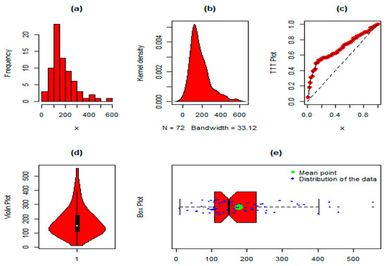
Figure 4. For dataset 1, the (a) histogram, (b) kernel density plot, (c) TTT plot, (d) violin plot, and (e) box plot.

Table 6. The ${\widehat{\mathit{\beta }}}_{\mathit{M}\mathit{L}\mathit{E}}$, ${\widehat{\mathit{\alpha }}}_{\mathit{M}\mathit{L}\mathit{E}}$, ${\widehat{\mathit{\delta }}}_{\mathit{M}\mathit{L}\mathit{E}}$, ${\widehat{\mathit{a}}}_{\mathit{M}\mathit{L}\mathit{E}}$, and ${\widehat{\mathit{b}}}_{\mathit{M}\mathit{L}\mathit{E}}$ values for infected guinea pigs data (dataset 1).

Models	${\widehat{\mathit{\beta }}}_{\mathit{M}\mathit{L}\mathit{E}}$	${\widehat{\mathit{\alpha }}}_{\mathit{M}\mathit{L}\mathit{E}}$	${\widehat{\mathit{\delta }}}_{\mathit{M}\mathit{L}\mathit{E}}$	${\widehat{\mathit{a}}}_{\mathit{M}\mathit{L}\mathit{E}}$	${\widehat{\mathit{b}}}_{\mathit{M}\mathit{L}\mathit{E}}$	${\widehat{\mathit{\theta }}}_{\mathit{M}\mathit{L}\mathit{E}}$
NGLog–Weib	0.014	0.978	9.322	-	-	-
APTra–Weib	0.003	6.818	1.190	-	-	-
NExpo–Weib	0.004	1.040	-	-	-	-
MO–Weib	0.002	1.243	-	-	-	2.372
FRL–Weib	0.003	1.223	-	-	-	8.160
Kumar–Weib	0.014	0.938	-	3.760	1.334	-

Table 7. The GFMs and p-values of the competing models for infected guinea pigs data (dataset 1).

Models	CM	AD	KS	p-Values
NGLog–Weib	0.079	0.092	0.086	0.665
APTra–Weib	0.804	0.138	0.171	0.029
NExpo–Weib	0.089	0.522	0.295	0.067
MO–Weib	0.161	0.941	0.173	0.027
FRLog–Weib	0.192	1.124	0.182	0.017
Kumar–Weib	0.082	0.523	0.092	0.580

Table 8. The DMs of the competing models for infected guinea pigs data (dataset 1).

Models	AIC	BIC	CAIC	HQIC
NGLog–Weib	856.654	863.485	857.007	859.373
APTra–Weib	864.127	870.957	864.479	866.846
NExpo–Weib	902.709	907.262	902.883	904.521
MO–Weib	865.711	872.541	866.064	868.430
FRLog–Weib	868.085	874.915	868.438	870.804
Kumar–Weib	859.492	868.599	860.089	863.117

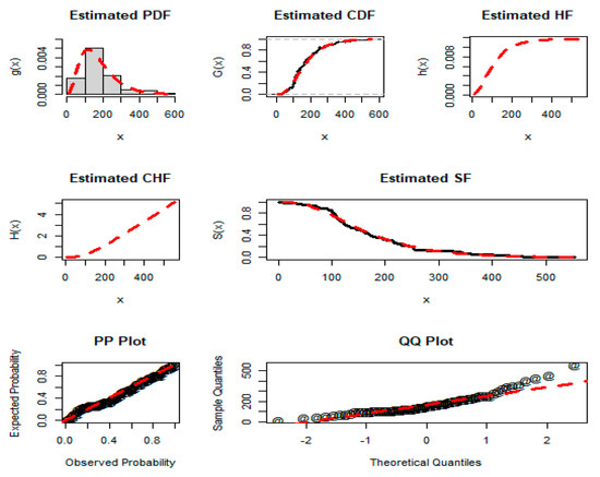
Figure 5. Estimated PDF, CDF, HF, CHF, SF, PP plot, and QQ plot of the NGLog–Weib distribution for dataset 1.

Given the results presented in Table 7 and Table 8, we can conclude that the NGLog–Weib distribution has the lowest GFM and DM values and the highest p-value, as compared to the other distributions. For the proposed NGLog–Weib distribution, the AMs are: CM = 0.079, AD = 0.492, KS = 0.086, AIC = 856.654, BIC = 863.484, CAIC = 857.007, HQIC = 859.373, and p-value = 0.665. In terms of the AD, KS, AIC, BIC, CAIC, HQIC, and p-value, the second cohesive distribution is the four-parameter Kumar–Weib model. For the Kumar–Weib model, the AM values of the KS, AIC, BIC, CAIC, HQIC, and p-value are given by 0.092, 859.492, 868.599, 860.089, 863.117, and 0.580, respectively, while in comparison to the AD, the second-best distribution is the three-parameter APTra–Weib model because for the APTra–Waib model, the value of the statistics, AD, is 0.138.

Hence, from the numerical depiction in Table 7 and Table 8, the visual graphical illustration (the close-fitting of the NGLog–Weib model), and the above comprehensive discussion, we can say that the newly derived NGLog–Weib model is a good competitor among the other compared probability models for the injected guinea pigs dataset.

6.2. Head and Neck Cancer, Dataset 2

The NGLog–Weib distribution was analysed on the head and neck cancer data and compared with the other distributions to evaluate its optimum fitting power. The summary measures were: min = 12.2, 1st quartile = 67.210, mean = 223.50, median = 128.50, 3rd quartile = 219.0, max = 1776.0, skewness = 3.384, kurtosis = 16.559, var = 93,286.41, and range = 1763.80. Some basic plots, such as the histogram, kernel density, TTT plot, violin plot, and box plot, for dataset 2 are presented in Figure 6. Similarly, the corresponding parameter values, i.e., ${\widehat{\beta }}_{MLE}$, ${\widehat{\alpha }}_{MLE}$, ${\widehat{\delta }}_{MLE}$, ${\widehat{a}}_{MLE}$, ${\widehat{b}}_{MLE}$, and ${\widehat{\theta }}_{MLE}$ of the NGLog–Weib distribution in comparison with the other competing probability distributions are given in Table 9, whereas the GFMs with p-values and DMs for selecting the best distribution of the competing probability distributions are presented in Table 10 and Table 11. Furthermore, the graphical representation, the estimated PDF, CDF, SF, PP, and QQ plots of the NGLog–Weib distribution, are shown in Figure 7.

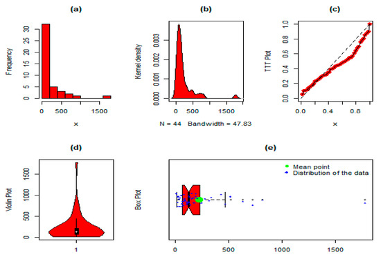
Figure 6. For dataset 2, the (a) histogram, (b) kernel density plot, (c) TTT plot, (d) violin plot, and (e) box plot.

Table 9. The ${\widehat{\mathit{\delta }}}_{\mathit{M}\mathit{L}\mathit{E}}$, ${\widehat{\mathit{\beta }}}_{\mathit{M}\mathit{L}\mathit{E}}$, ${\widehat{\mathit{\alpha }}}_{\mathit{M}\mathit{L}\mathit{E}}$, ${\widehat{\mathit{a}}}_{\mathit{M}\mathit{L}\mathit{E}}$, ${\widehat{\mathit{b}}}_{\mathit{M}\mathit{L}\mathit{E}}$ and ${\widehat{\mathit{\theta }}}_{\mathit{M}\mathit{L}\mathit{E}}$ for head and neck cancer data (dataset 2).

Models	${\widehat{\mathit{\beta }}}_{\mathit{M}\mathit{L}\mathit{E}}$	${\widehat{\mathit{\alpha }}}_{\mathit{M}\mathit{L}\mathit{E}}$	${\widehat{\mathit{\delta }}}_{\mathit{M}\mathit{L}\mathit{E}}$	${\widehat{\mathit{a}}}_{\mathit{M}\mathit{L}\mathit{E}}$	${\widehat{\mathit{b}}}_{\mathit{M}\mathit{L}\mathit{E}}$	${\widehat{\mathit{\theta }}}_{\mathit{M}\mathit{L}\mathit{E}}$
NGLog–Weib	0.707	0.325	53.292	-	-	-
APTra–Weib	0.003	0.245	0.993	-	-	-
NExpo–Weib	0.003	1.023	-	-	-	-
MO–Weib	0.003	1.001	-	-	-	0.508
FRL–Weib	0.029	0.762	-	-	-	5.722
Kumar–Weib	0.416	0.459	-	12.665	0.490	-

Table 10. The GFMs and p-values of the competing models for head and neck cancer data (dataset 2).

Models	CM	AD	KS	p-Values
NGLog–Weib	0.020	0.128	0.062	0.992
APTra–Weib	0.093	0.554	0.106	0.672
NExpo–Weib	0.087	0.515	0.101	0.727
MO–Weib	0.095	0.562	0.113	0.593
FRLog–Weib	0.191	1.096	0.134	0.379
Kumar–Weib	0.022	0.136	0.065	0.985

Table 11. The DMs of the competing models for head and neck cancer, dataset 2.

Models	AIC	BIC	CAIC	HQIC
NGLog–Weib	560.793	566.146	561.393	562.778
APTra–Weib	567.772	573.124	568.371	569.757
NExpo–Weib	565.157	568.725	565.450	566.480
MO–Weib	568.208	573.562	568.808	570.194
FRLog–Weib	572.884	578.236	573.484	574.869
Kumar–Weib	562.711	569.848	563.737	565.358

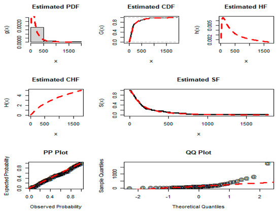
Figure 7. Estimated PDF, CDF, HF, CHF, SF, PP plot and QQ plot of the NGLog–Weib distribution for dataset 2.

The results presented in Table 10 and Table 11 show that the NGLog–Weib distribution has the lowest GFM and DM values and the highest p-value, as compared to the GFM and DM values and p-values of the other distributions. For the proposed NGLog–Weib distribution, the AMs and p-value are: CM = 0.018, AD = 0.119, KS = 0.057, AIC = 560.732, BIC = 566.085, CAIC = 561.332, HQIC = 562.717, and p-value = 0.9973, respectively. In terms of the CM, AD, KS, AIC, CAIC, HQIC, and p-value, the second optimum distribution is the Kumar–Weib model. For the Kumar–Weib model, the values of the CM, AD, KS, AIC, CAIC, HQIC, and p-value are given by 0.022, 0.136, 0.065, 562.711, 563.737, 565.358 and 0.985, respectively. Similarly, in terms of the BIC, the second optimum distribution is the NExpo–Weib distribution because its value is 568.725.

In light of the numerical justification in Table 10 and Table 11, the visual graphical illustration (the close-fitting of the proposed NGLog–Weib distribution) in Figure 7, and the above discussion, we can observe that the proposed NGLog–Weib distribution is a moral competitor among the other compared probability distributions for the head and neck cancer data (Data 2).

6.3. COVID−19 Patients, Dataset 3

The NGLog–Weib distribution was evaluated on the COVID-19 patients’ dataset. The key measures were: minimum = 1.516, 1st quartile = 2.788, mean = 3.282, median = 3.178, 3rd quartile = 3.637, maximum = 6.868, skewness = 3.384, kurtosis = 16.559, var = 93,286.41, and range = 1763.8. Figure 8 depicts the histogram, kernel density, TTT plot, violin plot, and box plot for the COVID-19 patients’ dataset 3. Similarly, the values of the parameters, i.e., ${\widehat{\beta }}_{MLE}$, ${\widehat{\alpha }}_{MLE}$, ${\widehat{\delta }}_{MLE}$, ${\widehat{a}}_{MLE}$, ${\widehat{b}}_{MLE}$, and ${\widehat{\theta }}_{MLE}$ of the NGLog–Weib model with the other competing probability distributions are displayed in Table 12, whereas the GFMs with p-values and DMs for selecting the best distribution of the competing distributions are recorded in Table 13 and Table 14. Furthermore, the graphical representation of the estimated PDF, CDF, SF, PP, and QQ plots of the NGLog–Weib distribution is shown in Figure 9.

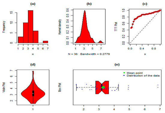
Figure 8. For dataset 3, the (a) histogram, (b) kernel density plot, (c) TTT plot, (d) violin plot, and (e) box plot.

Table 12. The ${\widehat{\mathit{\beta }}}_{\mathit{M}\mathit{L}\mathit{E}}$, ${\widehat{\mathit{\alpha }}}_{\mathit{M}\mathit{L}\mathit{E}}$, ${\widehat{\mathit{\delta }}}_{\mathit{M}\mathit{L}\mathit{E}}$, ${\widehat{\mathit{a}}}_{\mathit{M}\mathit{L}\mathit{E}}$, ${\widehat{\mathit{b}}}_{\mathit{M}\mathit{L}\mathit{E}}$ and ${\widehat{\mathit{\theta }}}_{\mathit{M}\mathit{L}\mathit{E}}$ values for COVID-19 data (dataset 3).

Models	${\widehat{\mathit{\beta }}}_{\mathit{M}\mathit{L}\mathit{E}}$	${\widehat{\mathit{\alpha }}}_{\mathit{M}\mathit{L}\mathit{E}}$	${\widehat{\mathit{\delta }}}_{\mathit{M}\mathit{L}\mathit{E}}$	${\widehat{\mathit{a}}}_{\mathit{M}\mathit{L}\mathit{E}}$	${\widehat{\mathit{b}}}_{\mathit{M}\mathit{L}\mathit{E}}$	${\widehat{\mathit{\theta }}}_{\mathit{M}\mathit{L}\mathit{E}}$
NGLog–Weib	0.477	1.481	22.931	-	-	-
APTra–Weib	0.206	171.542	1.954	-	-	-
NExpo–Weib	0.004	3.909	-	-	-	-
MO–Weib	0.039	2.833	-	-	-	1.928
FRLog–Weib	0.008	3.569	-	-	-	−0.544
Kumar–Weib	0.695	1.064	-	13.024	2.112	-

Table 13. The GFMs and p-values of the competing models for COVID-19 data (dataset 3).

Models	CM	AD	KS	p-Values
NGLog–Weib	0.092	0.536	0.106	0.813
APTra–Weib	0.103	0.582	0.123	0.649
NExpo–Weib	0.137	0.794	0.144	0.446
MO–Weib	0.182	1.035	0.141	0.474
FRL–Weib	0.163	0.937	0.148	0.411
Kumar–Weib	0.093	0.539	0.106	0.795

Table 14. The DMs of the competing models for COVID-19 data (dataset 3).

Models	AIC	BIC	CAIC	HQIC
NGLog–Weib	102.028	106.778	102.778	103.686
APTra–Weib	103.616	108.366	104.366	105.274
NExpo–Weib	104.294	107.461	104.657	105.399
MO–Weib	109.443	114.195	110.193	111.101
FRLog–Weib	108.532	113.283	109.282	110.190
Kumar–Weib	104.002	110.336	105.292	106.213

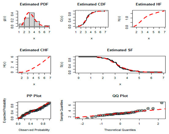
Figure 9. Estimated PDF, CDF, HF, CHF, SF, PP plot, and QQ plot of the NGLog–Weib distribution for dataset 3.

The results presented in Table 13 and Table 14 display that the NGLog–Weib distribution has the least GFM and DM values and highest p-values, as compared to the GFM and DM values and p-values of the other distributions. For the proposed NGLog–Weib distribution, the AMs and p-values are: CM = 0.092, AD = 0.536, KS = 0.104, AIC = 102.028, BIC = 106.778, CAIC = 102.778, HQIC = 103.686, and p-value = 0.813, respectively. In terms of the CM, AD, KS, and p-value, the second most optimum distribution is the Kumar–Weib model. For the Kumar–Weib model, the values of the CM, AD, KS, and p-value are 0.093, 0.539, 0.106, and 0.795, respectively. Similarly, in terms of the AIC, BIC, CAIC, and HQIC, the second-best distribution is the APTra–Weib distribution because it’s AIC, BIC, CAIC, and HQIC values are 103.616, 108.366, 104.366, and 105.274, respectively.

Based on the justification of the numerical description in Table 13 and Table 14, the visual graphical illustration in Figure 9, and the above comprehensive discussion, we can observe that the NGLog–Weib model is a good competitor among the other compared distributions for the COVID-19 dataset (Data 3).

6.4. Patients Receiving Analgesics, Dataset 4

Finally, the NGLog–Weib distribution was evaluated on the patients receiving analgesics’ datasets. The key measures were: minimum = 1.100, 1st quartile = 1.475, mean = 1.900, median = 1.700, 3rd quartile = 2.050, maximum = 4.100, skewness= 1.720, kurtosis= 5.924, var= 0.496, and range = 3.0. Figure 10 depicts the histogram, kernel density, TTT plot, violin plot, and box plot for patients receiving the analgesics, dataset 4. Similarly, the values of the parameters, i.e., ${\widehat{\beta }}_{MLE}$, ${\widehat{\alpha }}_{MLE}$, ${\widehat{\delta }}_{MLE}$, ${\widehat{a}}_{MLE}$, ${\widehat{b}}_{MLE}$, and ${\widehat{\theta }}_{MLE}$ of the NGLog–Weib, with other well-known competing distributions, are displayed in Table 15, whereas the GFMs with p-values and DMs for selecting the best distribution of the competing distributions are provided in Table 16 and Table 17. Furthermore, the graphical representation of the estimated PDF, CDF, SF, PP, and QQ plots of the NGLog–Weib distribution is shown in Figure 11.

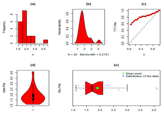
Figure 10. For dataset 4, the (a) histogram, (b) kernel density plot, (c) TTT plot, (d) violin plot, and (e) box plot.

Table 15. The ${\widehat{\mathit{\beta }}}_{\mathit{M}\mathit{L}\mathit{E}}$, ${\widehat{\mathit{\alpha }}}_{\mathit{M}\mathit{L}\mathit{E}}$, ${\widehat{\mathit{\delta }}}_{\mathit{M}\mathit{L}\mathit{E}}$, ${\widehat{\mathit{a}}}_{\mathit{M}\mathit{L}\mathit{E}}$, ${\widehat{\mathit{b}}}_{\mathit{M}\mathit{L}\mathit{E}}$ and ${\widehat{\mathit{\theta }}}_{\mathit{M}\mathit{L}\mathit{E}}$ values for the patients receiving analgesics’ data (dataset 4).

Models	${\widehat{\mathit{\beta }}}_{\mathit{M}\mathit{L}\mathit{E}}$	${\widehat{\mathit{\alpha }}}_{\mathit{M}\mathit{L}\mathit{E}}$	${\widehat{\mathit{\delta }}}_{\mathit{M}\mathit{L}\mathit{E}}$	${\widehat{\mathit{a}}}_{\mathit{M}\mathit{L}\mathit{E}}$	${\widehat{\mathit{b}}}_{\mathit{M}\mathit{L}\mathit{E}}$	${\widehat{\mathit{\theta }}}_{\mathit{M}\mathit{L}\mathit{E}}$
NGLog–Weib	2.091	1.009	78.683	-	-	-
APTra–Weib	0.021	0.016	3.620	-	-	-
NExpo–Weib	0.046	3.323	-	-	-	-
MO–Weib	0.003	4.408	-	-	-	0.044
FRLog–Weib	0.005	−0.986	-	-	-	4.828
Kumar–Weib	2.349	1.469	-	33.285	0.339	-

Table 16. The GFMs and p-values of the competing models for the patients receiving analgesics’ data (dataset 4).

Models	CM	AD	KS	p-Values
NGLog–Weib	0.058	0.344	0.146	0.850
APTra–Weib	0.132	0.779	0.158	0.701
NExpo–Weib	0.153	0.904	0.181	0.527
MO–Weib	0.076	0.457	0.165	0.802
FRLog–Weib	0.141	0.852	0.223	0.273
Kumar–Weib	0.060	0.359	0.156	0.833

Table 17. The DMs of the competing models for the patients receiving analgesics’ data (dataset 4).

Models	AIC	BIC	CAIC	HQIC
NGLog–Weib	38.699	41.687	40.199	39.282
APTra–Weib	43.418	46.404	44.917	44.000
NExpo–Weib	42.936	44.927	43.642	43.325
MO–Weib	40.781	43.769	42.283	41.363
FRLog–Weib	44.704	47.691	46.203	45.286
Kumar–Weib	39.924	43.907	42.591	40.702

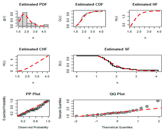
Figure 11. Estimated PDF, CDF, HF, CHF, SF, PP plot, and QQ plot of the NGLog–Weib distribution for dataset 4.

The results presented in Table 16 and Table 17 display that the NGLog–Weib distribution has the least AM values and the highest p-value, as compared to the AMs and p-values of the other distributions. For the proposed NGLog–Weib distribution, the AMs and p-value are: CM = 0.058, AD = 0.344, KS = 0.146, AIC = 38.699, BIC = 41.687, CAIC = 40.199, HQIC = 39.282, and p-value = 0.850, respectively. In terms of the CM, AD, KS, AIC, HQIC, and p-value, the second most optimum distribution is the Kumar–Weib model. For the Kumar–Weib model, the values of the CM, AD, KS, AIC, HQIC, and p-value are 0.060, 0.359, 0.156, 39.924, 40.702, and 0.833, respectively. Similarly, in terms of the BIC, CAIC, and HQIC, the second-best distribution is the MO–Weib model because its BIC, CAIC, and HQIC values are 43.768, 42.281, and 41.364, respectively.

Based on the justification of the numerical description in Table 16 and Table 17, the visual graphical illustration, and the above comprehensive discussion, we can observe that the proposed NGLog–Weib model is a good (or optimum) competitor among the other competing distributions for the patients receiving analgesics (dataset 4).

7. Conclusions

This study proposes a New Generalized Logarithmic-X (NGLog–X) family of distributions, which is a new family of continuous probability distributions. A three-parameter special subcase of the NGLog–X family of distributions was introduced by implementing the Weibull distribution as a baseline distribution. Various statistical and mathematical properties, such as the moments, moments generating function, residual life, reverse residual life, identifiability property, order statistics, and quantile function were investigated. To this end, the MLE method was utilized to estimate the unknown parameters of the NGLog–X family of distribution. A brief Monte Carlo simulation study was considered to check the efficiency of the ${\widehat{\delta }}_{MLE}$, ${\widehat{\alpha }}_{MLE}$, and ${\widehat{\beta }}_{MLE}$ of the NGLog–X family of distributions. The newly proposed method was applied to biomedical datasets in comparison to some other well-known distributions, including the APTra–Weib, MO–Weib, FRLog–Weib, NExpo–Weib, and Kumar–Weib distributions. Based on the GFMs and DMs, it is shown that the NGLog–Weib distribution provides a good fit in comparison with other competitive distributions by modelling the medical datasets. The results suggest that the proposed method and its generated models in distribution theory could provide useful applications in biomedical and other related fields.

References

- Liu, Y.; Ilyas, M.; Khosa, S.K.; Muhmoudi, E.; Ahmad, Z.; Khan, D.M.; Hamedani, G.G. A flexible reduced logarithmic-X family of distributions with biomedical analysis. Comput. Math. Methods Med. 2020, 2020, 4373595. [Google Scholar] [CrossRef] [PubMed]
- Almalki, S.J.; Yuan, J. A new modified Weibull distribution. Reliab. Eng. Syst. Saf. 2013, 111, 164–170. [Google Scholar] [CrossRef]
- Liao, Q.; Ahmad, Z.; Mahmoudi, E.; Hamedani, G.G. A new flexible bathtub-shaped modification of the Weibull model Properties and applications. Math. Probl. Eng. 2020, 2020, 3206257. [Google Scholar] [CrossRef]
- De Micheli, D.; Formigoni, M.L.O. Drug use by Brazilian students: Associations with family, psychosocial, health, demographic and behavioral characteristics. Addiction 2004, 99, 570–578. [Google Scholar] [CrossRef]
- Klakattawi, H.; Alsulami, D.; Elaal, M.A.; Dey, S.; Baharith, L. A new generalized family of distributions based on combining Marshal-Olkin transformation with TX family. PLoS ONE 2022, 17, e0263673. [Google Scholar] [CrossRef]
- Eghwerido, J.T.; Agu, F.I.; Ibidoja, O.J. The shifted exponential-G family of distributions: Properties and applications. J. Stat. Manag. Syst. 2022, 25, 43–75. [Google Scholar] [CrossRef]
- Kilai, M.; Waititu, G.A.; Kibira, W.A.; Alshanbari, H.M.; El-Morshedy, M. A new generalization of Gull Alpha Power Family of distributions with application to modeling COVID-19 mortality rates. Results Phys. 2022, 36, 105339. [Google Scholar] [CrossRef]
- Alkhairy, I.; Faqiri, H.; Shah, Z.; Alsuhabi, H.; Yusuf, M.; Aldallal, R.; Makumi, N.; Riad, F.H. A New Flexible Logarithmic-X Family of Distributions with Applications to Biological Systems. Complexity 2022, 2022, 7845765. [Google Scholar] [CrossRef]
- Tung, Y.L.; Ahmad, Z.; Mahmoudi, E. The Arcsine-X Family of Distributions with Applications to Financial Sciences. Comput. Syst. Sci. Eng. 2021, 39, 351–363. [Google Scholar] [CrossRef]
- Alzaatreh, A.; Aljarrah, M.A.; Smithson, M.; Shahbaz, S.H.; Shahbaz, M.Q.; Famoye, F.; Lee, C. Truncated family of distributions with applications to time and cost to start a business. Methodol. Comput. Appl. Probab. 2021, 23, 5–27. [Google Scholar] [CrossRef]
- Eghwerido, J.T.; Efe-Eyefia, E.; Zelibe, S.C. The transmuted alpha power-G family of distributions. J. Stat. Manag. Syst. 2021, 24, 965–1002. [Google Scholar] [CrossRef]
- Reyad, H.; Korkmaz, M.Ç.; Afify, A.Z.; Hamedani, G.G.; Othman, S. The Fréchet Topp Leone-G family of distributions: Properties, characterizations and applications. Ann. Data Sci. 2021, 8, 345–366. [Google Scholar] [CrossRef]
- Zichuan, M.; Hussain, S.; Iftikhar, A.; Ilyas, M.; Ahmad, Z.; Khan, D.M.; Manzoor, S. A new extended-family of distributions: Properties and applications. Comput. Math. Methods Med. 2020, 2020, 4650520. [Google Scholar] [CrossRef] [PubMed]
- Huo, X.; Khosa, S.K.; Ahmad, Z.; Almaspoor, Z.; Ilyas, M.; Aamir, M. A new lifetime exponential-X family of distributions with applications to reliability data. Math. Probl. Eng. 2020, 2020, 1316345. [Google Scholar] [CrossRef]
- Shah, Z.; Khan, D.M.; Khan, Z.; Shafiq, M.; Choi, J.G. A New Modified Exponent Power Alpha Family of Distributions with Applications in Reliability Engineering. Processes 2022, 10, 2250. [Google Scholar] [CrossRef]
- Hussain, S.; Rashid, M.S.; Ul Hassan, M.; Ahmed, R. The Generalized Alpha Exponent Power Family of Distributions: Properties and Applications. Mathematics 2022, 10, 1421. [Google Scholar] [CrossRef]
- Chen, P.; Ye, Z.S. Estimation of field reliability based on aggregate lifetime data. Technometrics 2017, 59, 115–125. [Google Scholar] [CrossRef]
- Xu, A.; Zhou, S.; Tang, Y. A unified model for system reliability evaluation under dynamic operating conditions. IEEE Trans. Reliab. 2019, 70, 65–72. [Google Scholar] [CrossRef]
- Zhang, L.; Xu, A.; An, L.; Li, M. Bayesian inference of system reliability for multicomponent stress-strength model under Marshall-Olkin Weibull distribution. Systems 2022, 10, 196. [Google Scholar] [CrossRef]
- Luo, C.; Shen, L.; Xu, A. Modelling and estimation of system reliability under dynamic operating environments and lifetime ordering constraints. Reliab. Eng. Syst. Saf. 2022, 218, 108136. [Google Scholar] [CrossRef]
- Zhuang, L.; Xu, A.; Wang, X.L. A prognostic driven predictive maintenance framework based on Bayesian deep learning. Reliab. Eng. Syst. Saf. 2023, 234, 109181. [Google Scholar] [CrossRef]
- Zhao, W.; Khosa, S.K.; Ahmad, Z.; Aslam, M.; Afify, A.Z. Type-I heavy tailed family with applications in medicine, engineering and insurance. PLoS ONE 2020, 15, e0237462. [Google Scholar] [CrossRef] [PubMed]
- Alzaatreh, A.; Famoye, F.; Lee, C. A new method for generating families of continuous distributions. Metron 2013, 71, 63–79. [Google Scholar] [CrossRef]
- Wang, Y.; Feng, Z.; Zahra, A. A new logarithmic family of distributions: Properties and applications. CMC-Comput. Mater. Contin. 2021, 66, 919–929. [Google Scholar]
- Zhao, Y.; Ahmad, Z.; Alrumayh, A.; Yusuf, M.; Aldallal, R.; Elshenawy, A.; Riad, F.H. A novel logarithmic approach to generate new probability distributions for data modeling in the engineering sector. Alex. Eng. J. 2023, 62, 313–325. [Google Scholar] [CrossRef]
- Eugene, N.; Lee, C.; Famoye, F. Beta-normal distribution and its applications. Commun. Stat.-Theory Methods 2002, 31, 497–512. [Google Scholar] [CrossRef]
- Zografos, K.; Balakrishnan, N. On families of beta-and generalized gamma-generated distributions and associated inference. Stat. Methodol. 2009, 6, 344–362. [Google Scholar] [CrossRef]
- Ristić, M.M.; Balakrishnan, N. The gamma-exponentiated exponential distribution. J. Stat. Comput. Simul. 2012, 82, 1191–1206. [Google Scholar] [CrossRef]
- Torabi, H.; Hedesh, N.M. The gamma-uniform distribution and its applications. Kybernetika 2012, 48, 16–30. [Google Scholar]
- Tahir, M.H.; Cordeiro, G.M.; Alzaatreh, A.; Mansoor, M.; Zubair, M. The logistic-X family of distributions and its applications. Commun. Stat.-Theory Methods 2016, 45, 7326–7349. [Google Scholar] [CrossRef]
- Ahmad, Z.; Mahmoudi, E.; Dey, S.; Khosa, S.K. Modeling vehicle insurance loss data using a new member of TX family of distributions. J. Stat. Theory Appl. 2020, 19, 133–147. [Google Scholar] [CrossRef]
- Shah, Z.; Ali, A.; Hamraz, M.; Khan, D.M.; Khan, Z.; EL-Morshedy, M.; Al-Bossly, A.; Almaspoor, Z. A New Member of TX Family with Applications in Different Sectors. J. Math. 2022, 2022, 1453451. [Google Scholar] [CrossRef]
- David, H.A. Order Statistics, 2nd ed.; Wiley: New York, NY, USA, 1981. [Google Scholar]
- Bjerkedal, T. Acquisition of Resistance in Guinea Pies infected with Different Doses of Virulent Tubercle Bacilli. Am. J. Hyg. 1960, 72, 130–148. [Google Scholar] [PubMed]
- Ceren, Ü.N.A.L.; Cakmakyapan, S.; Gamze, Ö.Z.E.L. Alpha power inverted exponential distribution: Properties and application. Gazi Univ. J. Sci. 2018, 31, 954–965. [Google Scholar]
- Almetwally, E.M.; Alharbi, R.; Alnagar, D.; Hafez, E.H. A new inverted topp-leone distribution: Applications to the COVID-19 mortality rate in two different countries. Axioms 2021, 10, 25. [Google Scholar] [CrossRef]
- Jamal, F.; Reyad, H.; Chesneau, C.; Nasir, M.A.; Othman, S. The Marshall-Olkin odd Lindley-G family of distributions: Theory and applications. Punjab Univ. J. Math. 2020, 51, 111–125. [Google Scholar]
- Dey, S.; Sharma, V.K.; Mesfioui, M. A new extension of Weibull distribution with application to lifetime data. Ann. Data Sci. 2017, 4, 31–61. [Google Scholar]
- Marshall, A.W.; Olkin, I. A new method for adding a parameter to a family of distributions with application to the exponential and Weibull families. Biometrika 1997, 84, 641–652. [Google Scholar] [CrossRef]
- Cordeiro, G.M.; Ortega, E.M.; Nadarajah, S. The Kumaraswamy Weibull distribution with application to failure data. J. Frankl. Inst. 2010, 347, 1399–1429. [Google Scholar] [CrossRef]
Disclaimer/Publisher’s Note: The statements, opinions and data contained in all publications are solely those of the individual author(s) and contributor(s) and not of MDPI and/or the editor(s). MDPI and/or the editor(s) disclaim responsibility for any injury to people or property resulting from any ideas, methods, instructions or products referred to in the content. |
© 2023 by the authors. Licensee MDPI, Basel, Switzerland. This article is an open access article distributed under the terms and conditions of the Creative Commons Attribution (CC BY) license (https://creativecommons.org/licenses/by/4.0/).