
Cloud Computing Considering Both Energy and Time Solved by Two-Objective Simplified Swarm Optimization


Abstract
1. Introduction
- An improved algorithm named two-objective simplified swarm optimization (tSSO) is developed in this work to revise and improve errors in the previous MOSSO algorithm [17], which ignores the fact that the number of temporary nondominated solutions is not always only one in the multi-objective problem, and some temporary nondominated solutions may not be temporary nondominated solutions in the next generation. The algorithm is based on SSO to deliver the job scheduling in cloud computing.
- More new algorithms, testing, and comparisons have been implemented to solve the bi-objective time-constrained task scheduling problem in a more efficient manner.
- In the experiments conducted, the proposed tSSO outperforms existing established algorithms, e.g., NSGA-II, MOPSO, and MOSSO, in the convergence, diversity, number of obtained temporary nondominated solutions, and the number of obtained real nondominated solutions.
2. Literature Review
2.1. A Review of Job Scheduling in Cloud-Computing
2.2. Algorithm Research for Solving the Single-Objective Problem for Job Scheduling in Cloud-Computing
2.3. Algorithm Research for Solving the Multi-Objective Problem for Job Scheduling in Cloud-Computing
3. Assumptions, and Mathematical Problem Description
3.1. Assumptions
- All jobs are available, independent, and equal in importance with two attributes, sizei and timei, for i = 1, 2, …, Nvar for processing simultaneously at time zero.
- Each processor is available at any time with two attributes, denoted as speedj and powerj, j = 1, 2, …, Ncpu, and cannot process two or more jobs simultaneously.
- All processing times include set-up time.
- Job pre-emption and the splitting of jobs are not permitted.
- There is an infinite buffer between the processors.
3.2. The Mathematical Model
4. SSO, Crowding Distance, and Elite Selection
4.1. Simplified Swarm Optimization
- STEP S0.
- Generate Xi randomly, find gBest, and let t = 1, k = 1, and Pi = Xi for i = 1, 2, …, Nsol.
- STEP S1.
- Update Xk.
- STEP S2.
- If F(Xk) is better than F(Pk), let Pk = Xk. Otherwise, go to STEP S5.
- STEP S3.
- If F(Pk) is better than F(PgBest), let gBest = k.
- STEP S4.
- If k < Nsol, let k = k + 1 and go to STEP S1.
- STEP S5.
- If t < Ngen, let t = t + 1, k = 1, and go to STEP S1. Otherwise, halt.
4.2. Crowding Distance
4.3. The Elite Selection
5. Proposed Algorithm
5.1. Purpose of tSSO
- The novel update mechanism of the role of gBest and pBest in the proposed tSSO, which are introduced in Section 5.3.
- The hybrid elite selection in the proposed tSSO, which is introduced in Section 5.4.
5.2. Solution Structure
5.3. Novel Update Mechanism
5.4. Hybrid Elite Selection
5.5. Group Comparison
5.6. Proposed tSSO
- STEP 0.
- Create initial population Xi randomly for i = 1, 2, …, Nsol and let t = 2.
- STEP 1.
- Let πt be all temporary nondominated solutions in S* = {Xk | for k = 1, 2, …, 2Nsol} and XNsol+k is updated from Xk based on Equation (8) for k = 1, 2, …, Nsol.
- STEP 2.
- If Nsol ≤ |πt|, let S = {top Nsol solutions in πt based on crowding distances} and go to STEP 4.
- STEP 3.
- Let S = πt ∪ {Nsol − |πt| solutions selected randomly from S* − πt}.
- STEP 4.
- Re-index these solutions in S such that S = {Xk|for k = 1, 2, …, Nsol}.
- STEP 5.
- If t < Ngen, then let t = t + 1 and go back to STEP 1. Otherwise, halt.
6. Simulation Results and Discussion
6.1. Parameter-Settings
6.2. Experimental Environments
- Each processor speed is generated between 1000 and 10,000 (MIPs) randomly, and the largest speed is ten times the smallest one.
- The power consumptions grow polynomial as the speed of processors grow, and the value range is between 0.3 and 30 (KW) per unit time.
- The values of job sizes are between 5000 and 15,000 (MIs).
6.3. Performance Metrics
6.4. Numerical Results
- The lower the cr value, the better the performance. In the small-size problem, the proposed tSSO7 with cp = 0.5 and cw = 0.3 is the best among all 12 algorithms. However, the proposed tSSO8 with cp = 0.5 and cw = 0.5 is the best one for the medium- and large-size problems. The reason for this is that the number of real nondominated solutions is infinite. Even though in the update mechanism of the proposed tSSO when cr = 0 there is only an exchange of information between the current solution itself and one of selected temporary nondominated solutions, it is already able to update the current solution to a better solution without needing any random movement.
- The larger the size of the problem, e.g., Njob, the fewer the number of obtained nondominated solutions, e.g., Nn and Np. There are two reasons why this is the case: (1) due to the characteristic of the NP-hard problems, i.e., the larger the size of the NP-hard problem, the more difficult it is to solve; (2) it is more difficult to find nondominated solutions for larger problems with the same deadline of 30 for all problems.
- The larger the Nsol, the more likely it is to find more nondominated solutions, i.e., the larger Nn and Np for the best algorithm among these algorithms no matter the size of the problem. Hence, it is an effective method to have a larger value of Nsol if we intend to find more nondominated solutions.
- The smaller the Njob, the fewer the number of obtained nondominated solutions, e.g., There are two reasons for the above: (1) due to the characteristic of the NP-hard problems, i.e., the larger the size of the NP-hard problem, the more difficult it is to solve; (2) it is more difficult to find nondominated solutions for larger problems with the same deadline, which is set 30 for all problems.
- The smaller the value of Np, the shorter the run time. The most time-consuming aspect of finding nondominated solutions is filtering out these nondominated solutions from current solutions. Hence, a new method, called the group comparison, is proposed in this study to find these nondominated solutions from current solutions. However, even the proposed group comparison is more efficient than the traditional pairwise comparison on average, but it still needs O(Np2) to achieve the goal.
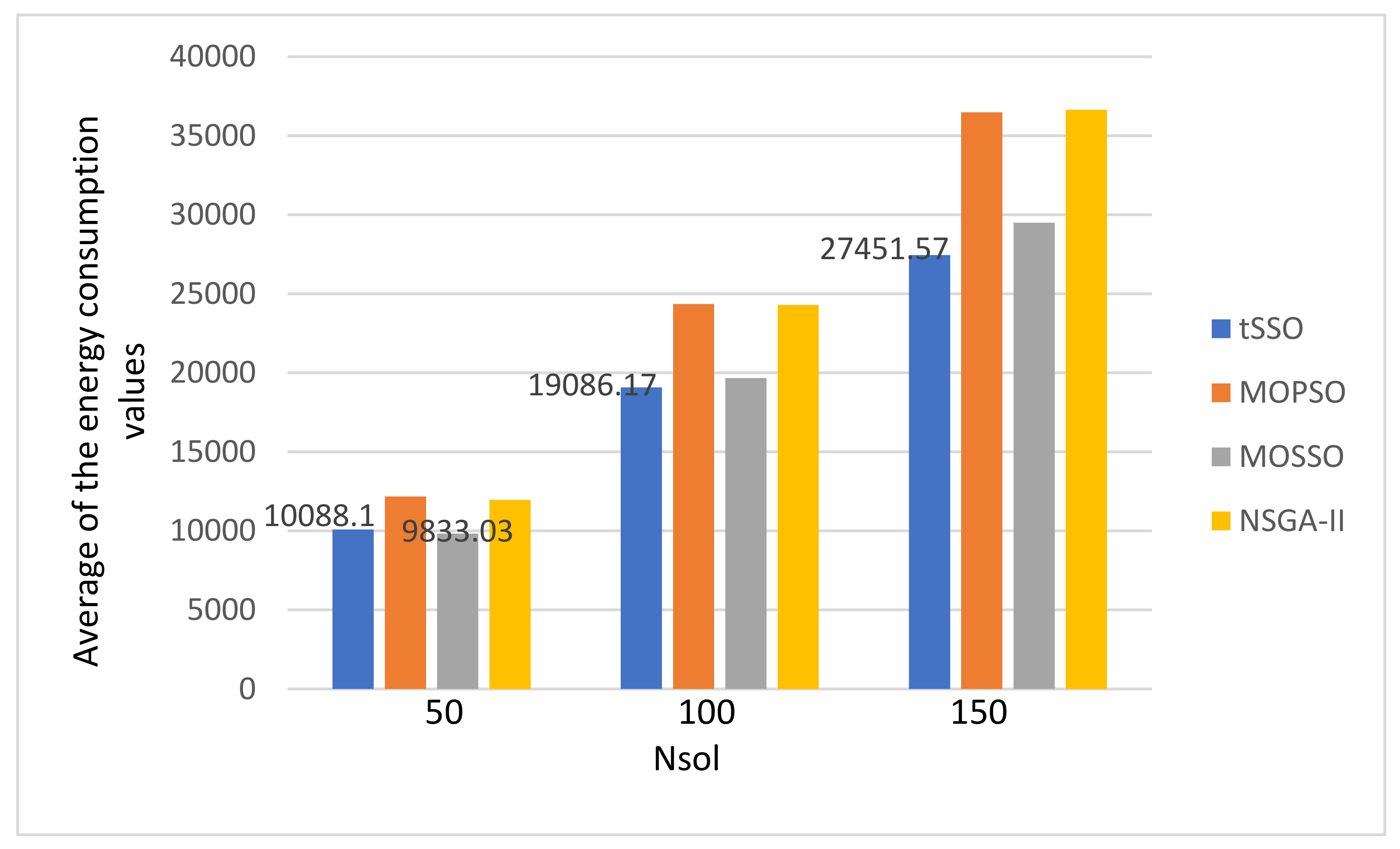
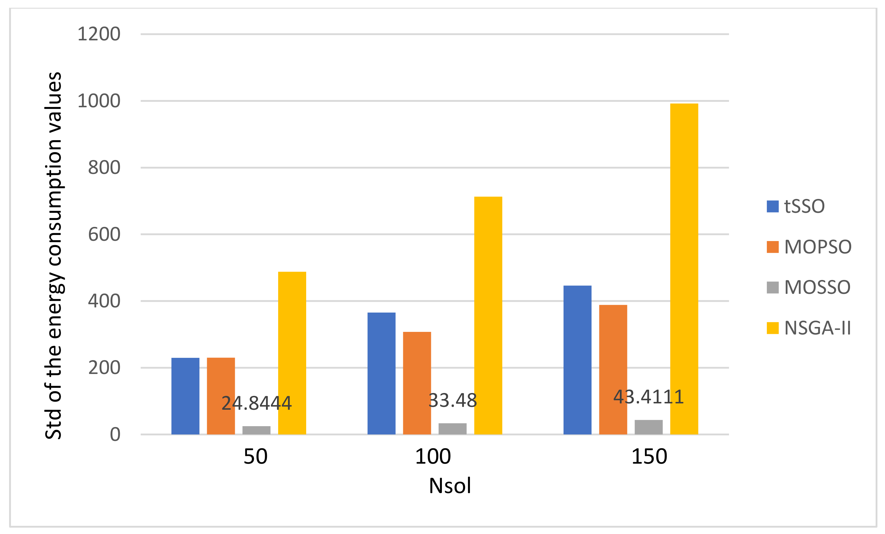
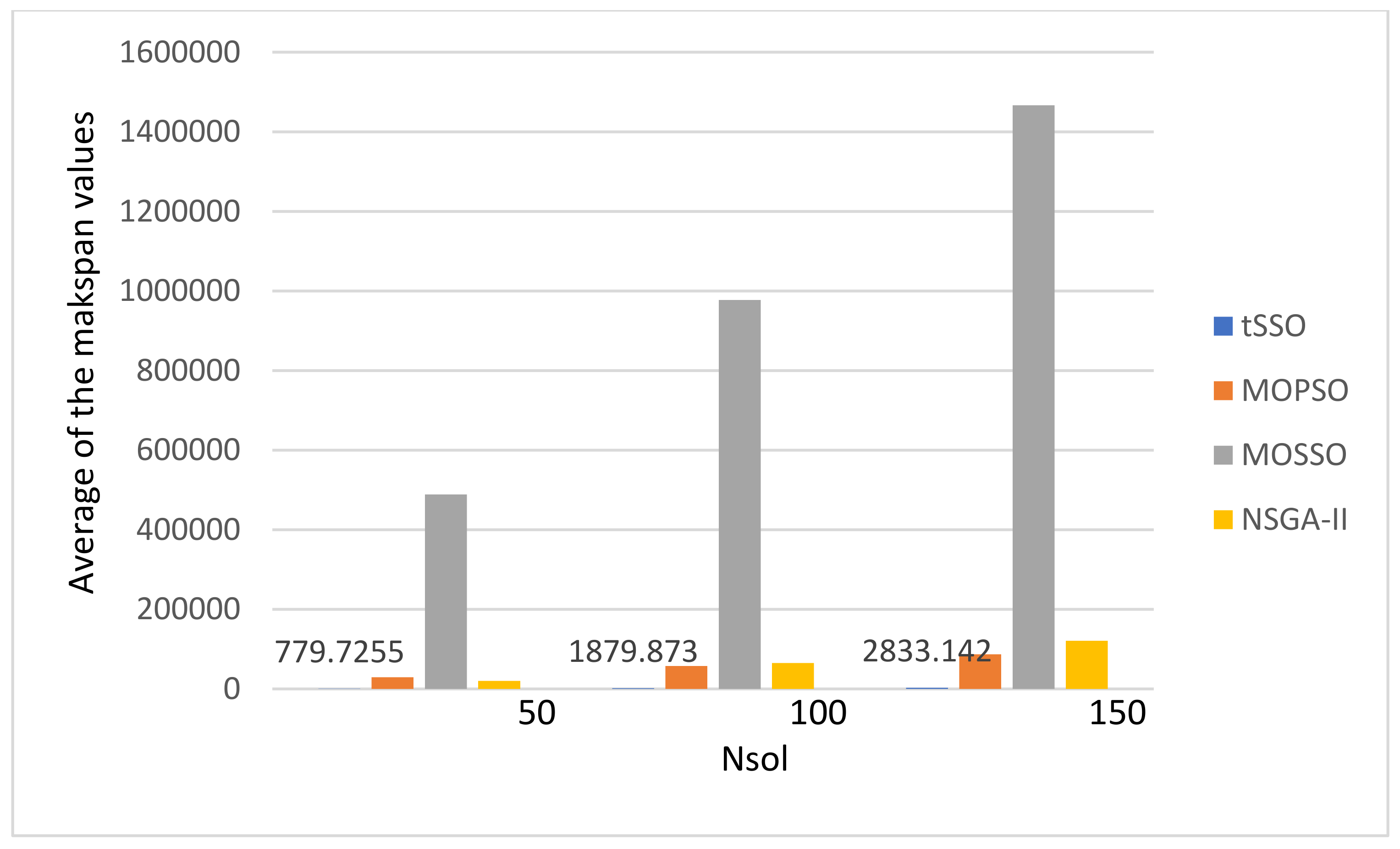
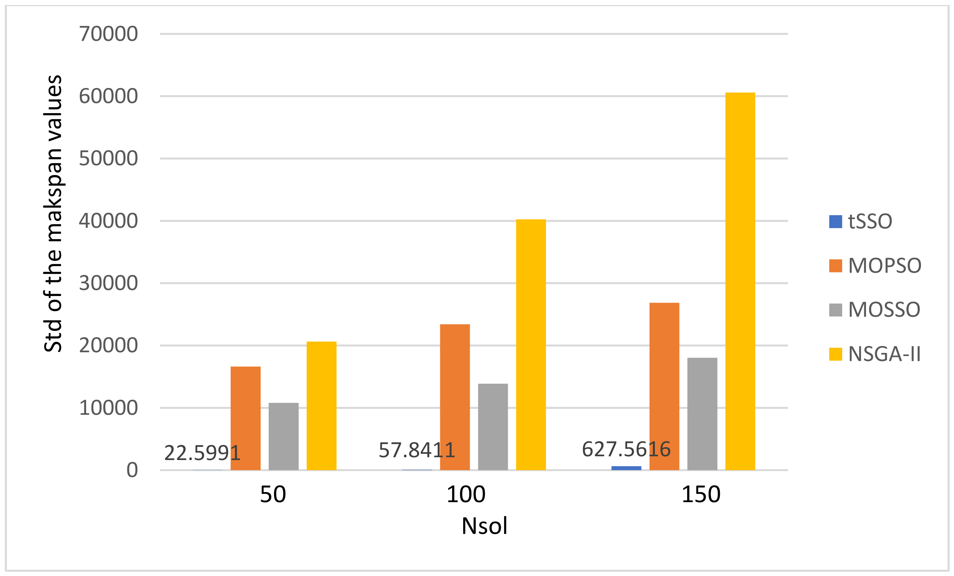
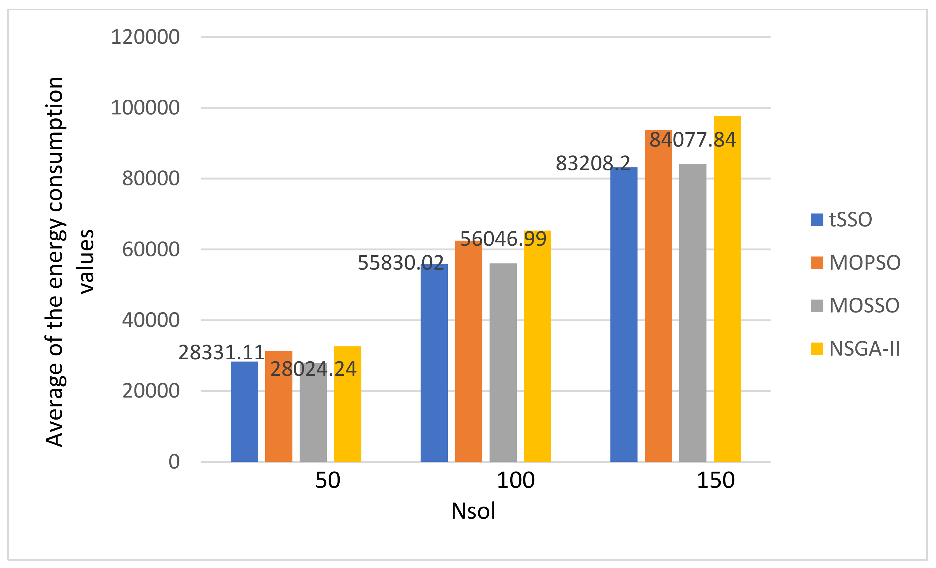
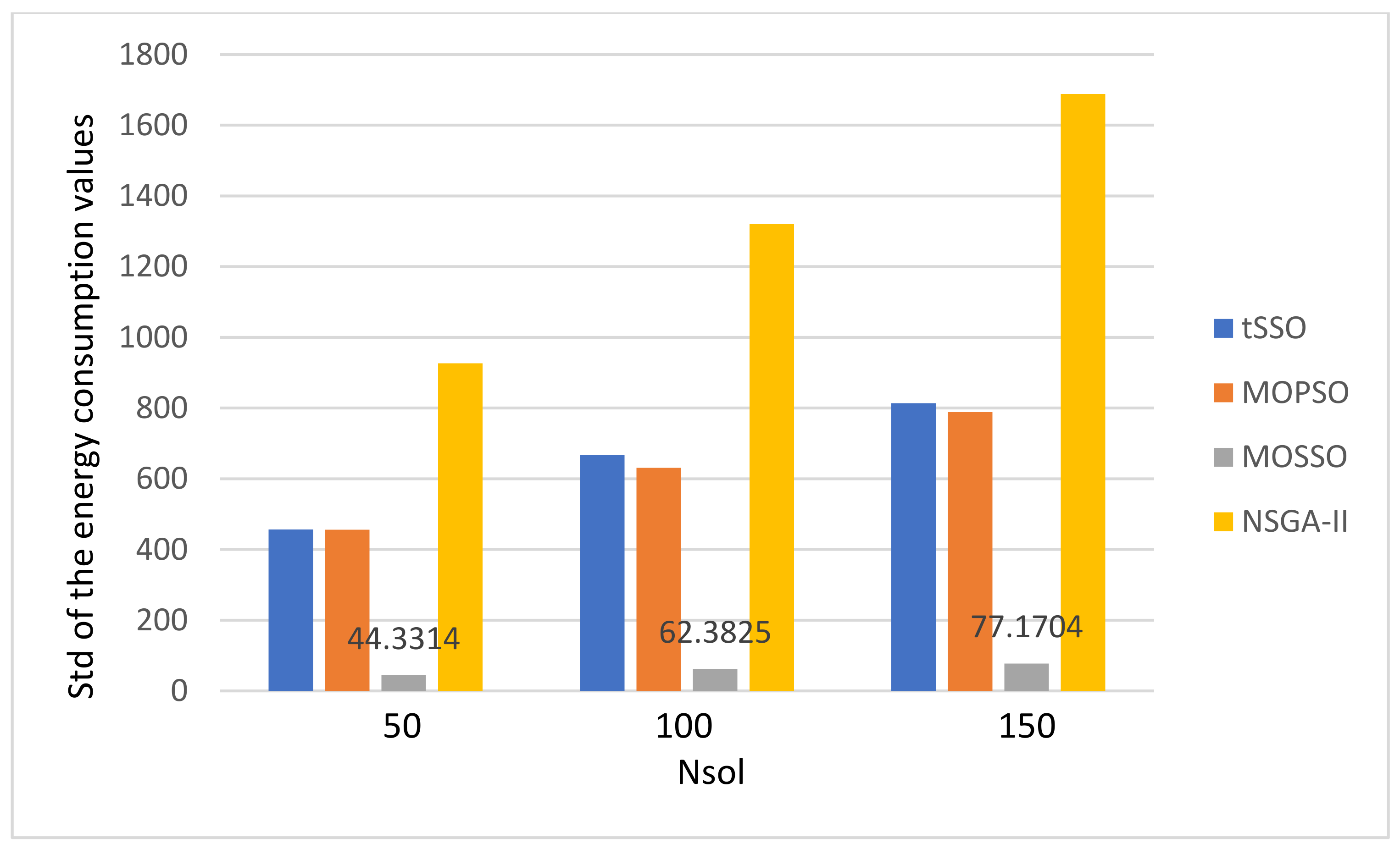
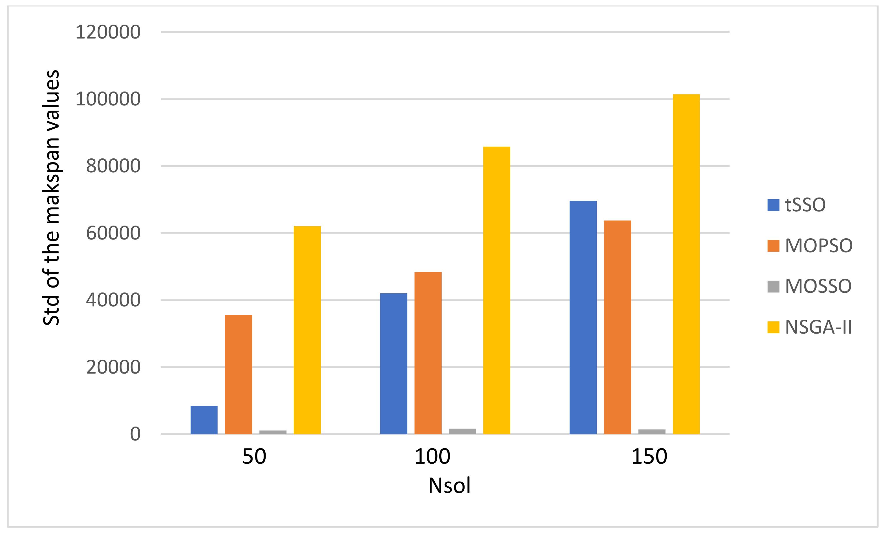
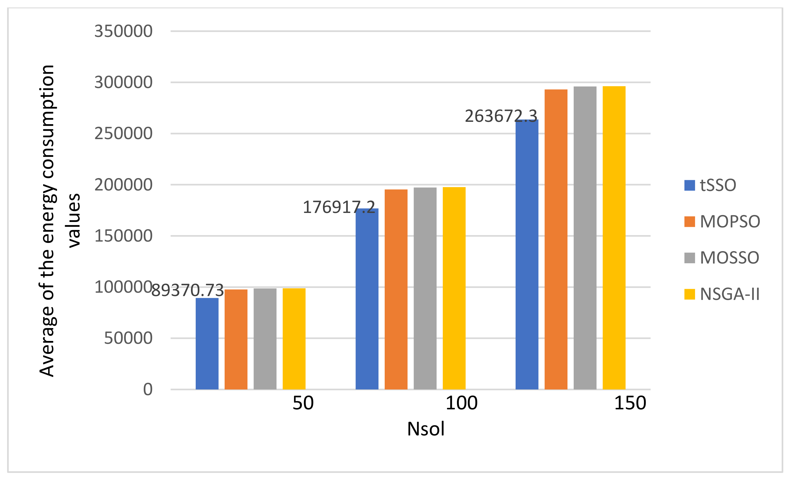
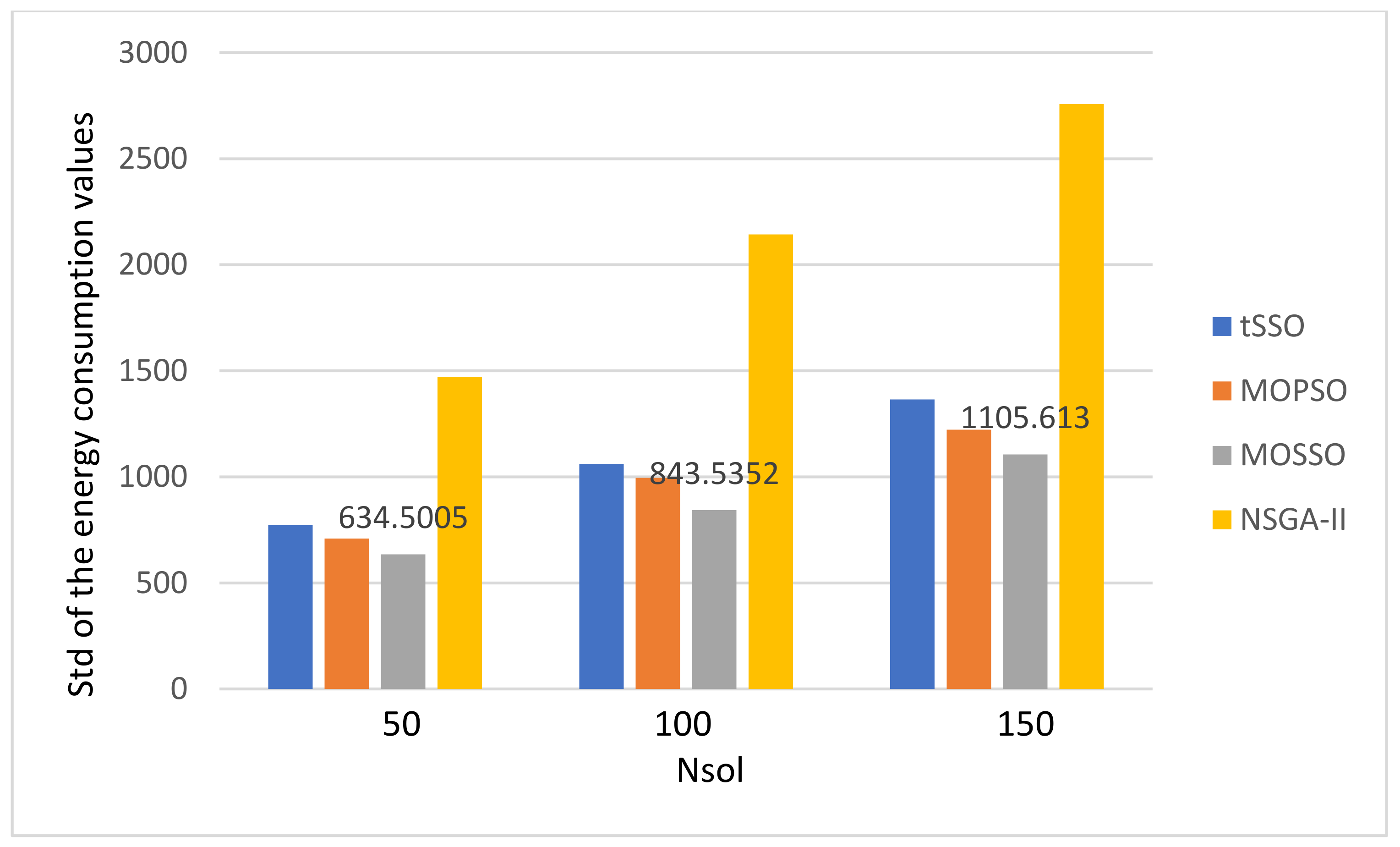
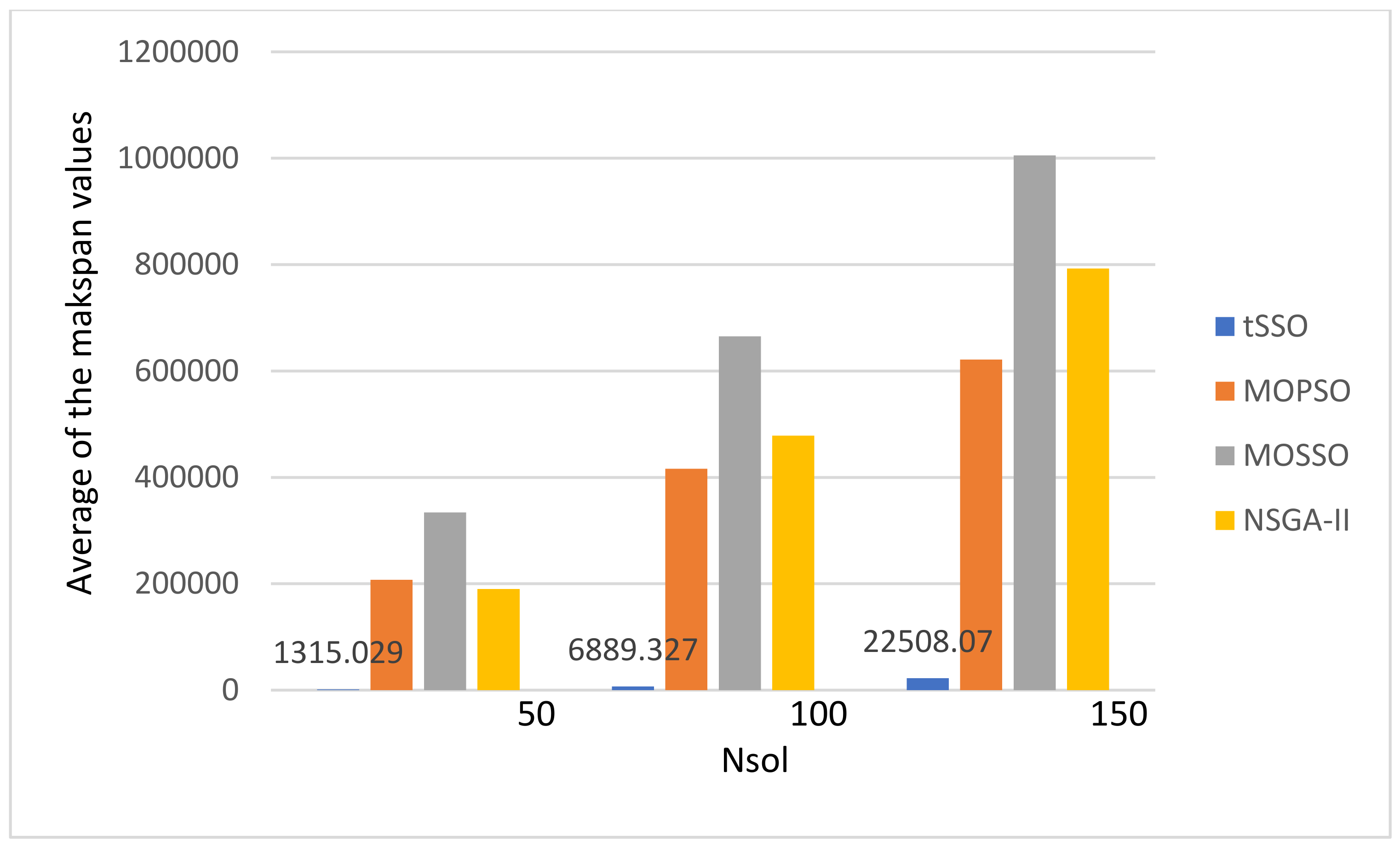
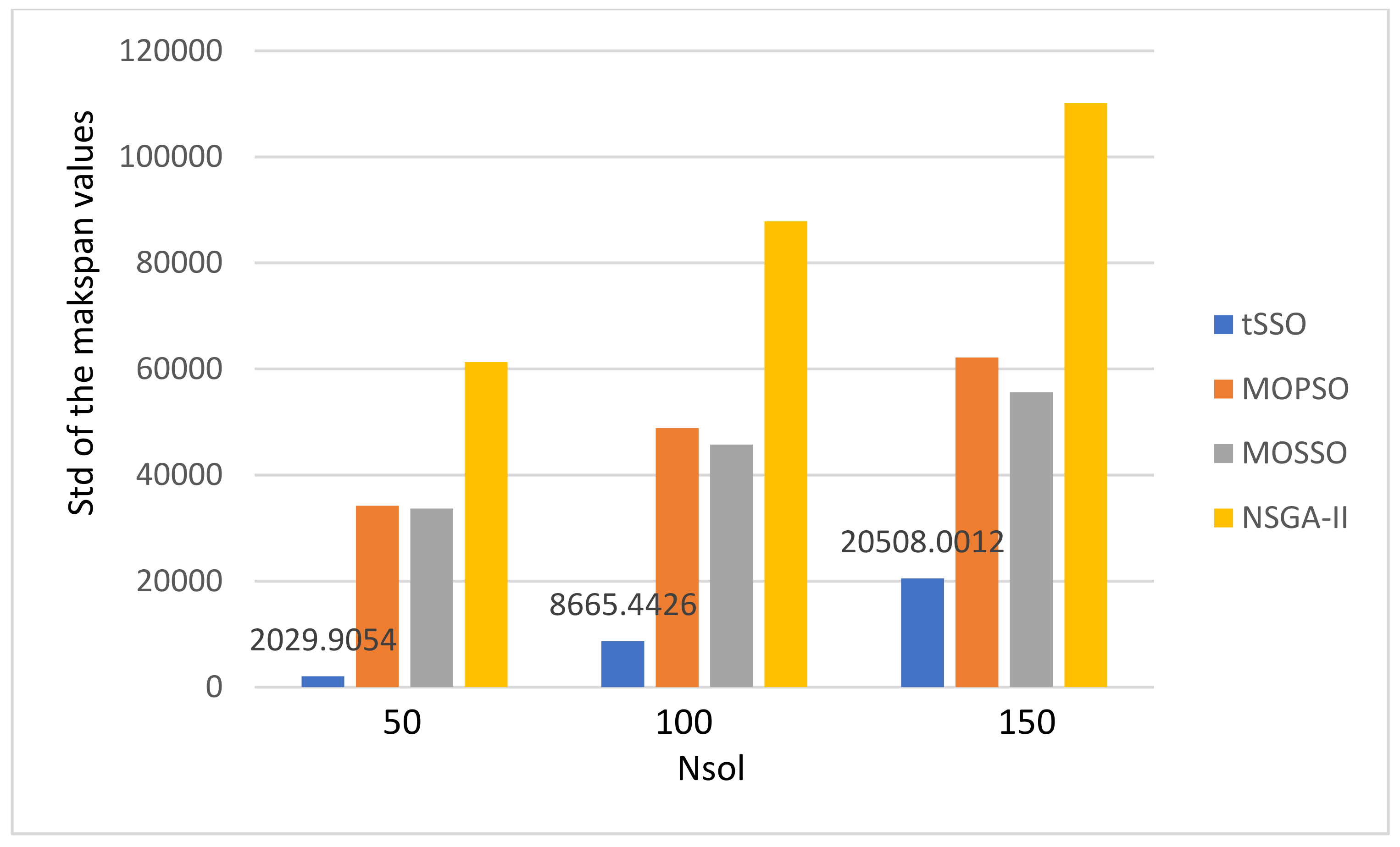
- There is no special pattern in solution qualities, e.g., the value of GD, SP, Nn, and Np, from the final average values of the energy consumption and the makspan.
- The one with the better number of obtained nondominated solutions also has better DP and SP values.
- The MOPSO [13] and the original MOSSO [17] share one common factor: each solution must inherit and update based on its predecessor (parent) and its pBest, and this is the main reason that it is less likely to find new nondominated solutions. The above observation is coincident to that observed in item 1. Hence, the proposed tSSO and the NSGA-II [19,20] are much better than MOSSO [17] and MOPSO [13] in solution quality.
7. Conclusions
Author Contributions
Funding
Acknowledgments
Conflicts of Interest
Notations
| |●| | number of elements in ● |
| Nvar | number of jobs used in the test problem |
| Ncpu | number of processors contained in the given data center |
| Nrun | number of runs for the algorithms |
| Ngen | number of generations in each run |
| Nsol | number of solutions in each generation |
| Nnon | number of selected temporary nondominated solutions |
| Xi | ith solution |
| xi,j | jth variable in Xi |
| Pi | the best solution among all solutions updated based on Xi in SSO |
| pi,j | jth variable in Pi |
| gBest | index of the best solution among all solutions in SSO, i.e., F(PgBest) is better than or equal to F(Pi) for i = 1, 2, …, Nsol |
| ρI | random number generated uniformly within interval I |
| cg, cp, cw, cr | positive parameters used in SSO with cg + cp + cw + cr = 1 |
| Cg, Cp, Cw | Cg = cg, Cp = Cg + cp, and Cw = Cp + cw |
| Fl(●) | lth fitness function value of solution ● |
| Max(●) | maximal value of ●, i.e., Max(Fl) is the maximal value of the lth objective function |
| Min(●) | minimal value of ●, i.e., Min(Fl) is the minimal value of the lth objective function |
| St | set of selected solutions from Πt to generate new solutions in the (t + 1)th generation. Note that S1 = Π1 and |St| = Nsol for i = 1, 2, …, Ngen |
| sizei | size of the job i for i = 1, 2, …, Nvar |
| starti | start time of the job i for i = 1, 2, …, Nvar |
| speedj | execution speed of the processor j for j = 1, 2, …, Ncpu |
| ej | energy consumption per unit time of the processor j for j = 1, 2, …, Ncpu |
| Tub | deadline constraint of job scheduling |
| ti,j | processing time ti,j where for i = 1, 2, …, Nvar and j = 1, 2, …, Ncpu |
References
- Wang, F.; Xu, J.; Cui, S. Optimal Energy Allocation and Task Offloading Policy for Wireless Powered Mobile Edge Computing Systems. IEEE Trans. Wirel. Commun. 2020, 19, 2443–2459. [Google Scholar] [CrossRef]
- Wei, S.C.; Yeh, W.C. Resource allocation decision model for dependable and cost-effective grid applications based on Grid Bank. Future Gener. Comput. Syst. 2017, 77, 12–28. [Google Scholar] [CrossRef]
- Yeh, W.C.; Wei, S.C. Economic-based resource allocation for reliable Grid-computing service based on Grid Bank. Future Gener. Comput. Syst. 2012, 28, 989–1002. [Google Scholar] [CrossRef]
- Manikandan, N.; Gobalakrishnan, N.; Pradeep, K. Bee optimization based random double adaptive whale optimization model for task scheduling in cloud computing environment. Comput. Commun. 2022, 187, 35–44. [Google Scholar] [CrossRef]
- Guo, W.; Li, J.; Chen, G.; Niu, Y.; Chen, C. A PSO-Optimized Real-Time Fault-Tolerant Task Allocation Algorithm in Wireless Sensor Networks. IEEE Trans. Parallel Distrib. Syst. 2015, 26, 3236–3249. [Google Scholar] [CrossRef]
- Afifi, H.; Horbach, K.; Karl, H. A Genetic Algorithm Framework for Solving Wireless Virtual Network Embedding. In Proceedings of the 2019 International Conference on Wireless and Mobile Computing, Networking and Communications (WiMob), Barcelona, Spain, 21–23 October 2019. [Google Scholar]
- Santos, J.; Hempel, M.; Sharif, H. Compression Distortion-Rate Analysis of Biomedical Signals in Machine Learning Tasks in Biomedical Wireless Sensor Network Applications. In Proceedings of the 2020 International Wireless Communications and Mobile Computing (IWCMC), Limassol, Cyprus, 15–19 June 2020. [Google Scholar]
- Sun, Z.; Liu, Y.; Tao, L. Attack Localization Task Allocation in Wireless Sensor Networks Based on Multi-Objective Binary Particle Swarm Optimization. J. Netw. Comput. Appl. 2018, 112, 29–40. [Google Scholar] [CrossRef]
- Lu, Y.; Zhou, J.; Xu, M. Wireless Sensor Networks for Task Allocation using Clone Chaotic Artificial Bee Colony Algorithm. In Proceedings of the 2019 IEEE International Conference of Intelligent Applied Systems on Engineering (ICIASE), Fuzhou, China, 26–29 April 2019. [Google Scholar]
- Khan, M.S.A.; Santhosh, R. Task scheduling in cloud computing using hybrid optimization algorithm. Soft Comput. 2022, 26, 3069–13079. [Google Scholar] [CrossRef]
- Malawski, M.; Juve, G.; Deelman, E.; Nabrzyski, J. Algorithms for cost-and deadline-constrained provisioning for scientific workflow ensembles in IaaS clouds. Future Gener. Comput. Syst. 2015, 48, 1–18. [Google Scholar] [CrossRef]
- Chen, H.; Zhu, X.; Guo, H.; Zhu, J.; Qin, X.; Wu, J. Towards energy-efficient scheduling for real-time tasks under uncertain cloud computing environment. J. Syst. Softw. 2015, 99, 20–35. [Google Scholar] [CrossRef]
- Coello, C.A.C.; Pulido, G.T.; Lechuga, M.S. Handling multiple objectives with particle swarm optimization. IEEE Trans. Evol. Comput. 2004, 8, 256–279. [Google Scholar] [CrossRef]
- Guo, X. Multi-objective task scheduling optimization in cloud computing based on fuzzy self-defense algorithm. Alex. Eng. J. 2021, 60, 5603–5609. [Google Scholar] [CrossRef]
- Liu, J.X.; Luo, G.; Zhang, X.M.; Zhang, F.; Li, B.N. Job scheduling model for cloud computing based on multi-objective genetic algorithm. Int. J. Comput. Sci. Issues 2013, 10, 134–139. [Google Scholar]
- Jena, R.K. Multi objective task scheduling in cloud environment using nested PSO framework. Procedia Comput. Sci. 2015, 57, 1219–1227. [Google Scholar] [CrossRef]
- Huang, C.L.; Jiang, Y.Z.; Yin, Y.; Yeh, W.C.; Chung, V.Y.Y.; Lai, C.M. Multi Objective Scheduling in Cloud Computing Using MOSSO. In Proceedings of the 2018 IEEE Congress on Evolutionary Computation (CEC), Rio de Janeiro, Brazil, 8–13 July 2018. [Google Scholar] [CrossRef]
- Yeh, W.C. A two-stage discrete particle swarm optimization for the problem of multiple multi-level redundancy allocation in series systems. Expert Syst. Appl. 2009, 36, 9192–9200. [Google Scholar] [CrossRef]
- Deb, K.; Pratap, A.; Agarwal, S.; Meyarivan, T. A fast and elitist multiobjective genetic algorithm: NSGA-II. IEEE Trans. Evol. Comput. 2002, 6, 182–197. [Google Scholar] [CrossRef]
- Yeh, W.C.; Zhu, W.; Yin, Y.; Huang, C.L. Cloud computing task scheduling problem by Nondominated Sorting Genetic Algorithm II (NSGA-II). In Proceedings of the First Australian Conference on Industrial Engineering and Operations Management, Sydney, Australia, 20–22 December 2022. [Google Scholar]
- Houssein, E.H.; Gad, A.G.; Wazery, Y.M.; Suganthan, P.N. Task Scheduling in Cloud Computing based on Meta-heuristics: Review, Taxonomy, Open Challenges, and Future Trends. Swarm Evol. Comput. 2021, 62, 100841. [Google Scholar] [CrossRef]
- Arunarani, A.R.; Manjul, D.; Sugumaran, V. Task scheduling techniques in cloud computing: A literature survey. Future Gener. Comput. Syst. 2019, 91, 407–415. [Google Scholar] [CrossRef]
- Kumar, M.; Sharma, S.C.; Goel, A.; Singh, S.P. A comprehensive survey for scheduling techniques in cloud computing. J. Netw. Comput. Appl. 2019, 143, 1–33. [Google Scholar] [CrossRef]
- Chen, X.; Cheng, L.; Liu, C.; Liu, Q.; Liu, J.; Mao, Y.; Murphy, J. A WOA-Based Optimization Approach for Task Scheduling in Cloud Computing Systems. IEEE Syst. J. 2020, 14, 3117–3128. [Google Scholar] [CrossRef]
- Attiya, I.; Elaziz, M.A.; Xiong, S. Job Scheduling in Cloud Computing Using a Modified Harris Hawks Optimization and Simulated Annealing Algorithm. Comput. Intell. Neurosci. 2020, 2020, 3504642. [Google Scholar] [CrossRef]
- Gąsior, J.; Seredyński, F. Security-Aware Distributed Job Scheduling in Cloud Computing Systems: A Game-Theoretic Cellular Automata-Based Approach. In Proceedings of the International Conference on Computational Science ICCS 2019: Computational Science—ICCS; 2019; pp. 449–462. [Google Scholar]
- Mansouri, N.; Javidi, M.M. Cost-based job scheduling strategy in cloud computing environments. Distrib. Parallel Databases 2020, 38, 365–400. [Google Scholar] [CrossRef]
- Cheng, F.; Huang, Y.; Tanpure, B.; Sawalani, P.; Cheng, L.; Liu, C. Cost-aware job scheduling for cloud instances using deep reinforcement learning. Clust. Comput. 2022, 25, 619–631. [Google Scholar] [CrossRef]
- Shukri, S.E.; Al-Sayyed, R.; Hudaib, A.; Mirjalili, S. Enhanced multi-verse optimizer for task scheduling in cloud computing environments. Expert Syst. Appl. 2021, 168, 114230. [Google Scholar] [CrossRef]
- Jacob, T.P.; Pradeep, K. A Multi-objective Optimal Task Scheduling in Cloud Environment Using Cuckoo Particle Swarm Optimization. Wirel. Pers. Commun. 2019, 109, 315–331. [Google Scholar] [CrossRef]
- Abualigah, L.; Diabat, A. A novel hybrid antlion optimization algorithm for multi-objective task scheduling problems in cloud computing environments. Clust. Comput. 2021, 24, 205–223. [Google Scholar] [CrossRef]
- Sanaj, M.S.; Prathap, P.M.J. Nature inspired chaotic squirrel search algorithm (CSSA) for multi objective task scheduling in an IAAS cloud computing atmosphere. Eng. Sci. Technol. Int. J. 2020, 23, 891–902. [Google Scholar] [CrossRef]
- Abualigah, L.; Alkhrabsheh, M. Amended hybrid multi-verse optimizer with genetic algorithm for solving task scheduling problem in cloud computing. J. Supercomput. 2022, 78, 740–765. [Google Scholar] [CrossRef]
- Mitchell, M. An Introduction to Genetic Algorithms; MIT Press: London, UK, 1998. [Google Scholar]
- Yeh, W.C. Orthogonal simplified swarm optimization for the series–parallel redundancy allocation problem with a mix of components. Knowl.-Based Syst. 2014, 64, 1–12. [Google Scholar] [CrossRef]
- Yeh, W.C. A New Exact Solution Algorithm for a Novel Generalized Redundancy Allocation Problem. Inf. Sci. 2017, 408, 182–197. [Google Scholar] [CrossRef]
- Yeh, W.C.; Hsieh, Y.H.; Hsu, K.Y.; Huang, C.L. ANN and SSO Algorithms for a Newly Developed Flexible Grid Trading Model. Electronics 2022, 11, 11193259. [Google Scholar] [CrossRef]
- Yeh, W.C. Simplified swarm optimization in disassembly sequencing problems with learning effects. Comput. Oper. Res. 2012, 39, 2168–2177. [Google Scholar] [CrossRef]
- Yeh, W.C. New parameter-free simplified swarm optimization for artificial neural network training and its application in the prediction of time series. IEEE Trans. Neural Netw. Learn. Syst. 2013, 24, 661–665. [Google Scholar] [PubMed]
- Yeh, W.C.; Zhu, W.; Peng, Y.F.; Huang, C.L. A Hybrid Algorithm Based on Simplified Swarm Optimization for Multi-Objective Optimizing on Combined Cooling, Heating and Power System. Appl. Sci. 2022, 12, 10595. [Google Scholar] [CrossRef]
- Yeh, W.C.; Huang, C.L.; Lin, P.; Chen, Z.; Jiang, Y.; Sun, B. Simplex Simplified Swarm Optimization for the Efficient Optimization of Parameter Identification for Solar Cell Models. IET Renew. Power Gener. 2018, 12, 45–51. [Google Scholar] [CrossRef]
- Yeh, W.C.; Ke, Y.C.; Chang, P.C.; Yeh, Y.M.; Chung, V. Forecasting Wind Power in the Mai Liao Wind Farm based on the Multi-Layer Perceptron Artificial Neural Network Model with Improved Simplified Swarm Optimization. Int. J. Electr. Power Energy Syst. 2014, 55, 741–748. [Google Scholar] [CrossRef]
- Yeh, W.C.; Liu, Z.; Yang, Y.C.; Tan, S.Y. Solving Dual-Channel Supply Chain Pricing Strategy Problem with Multi-Level Programming Based on Improved Simplified Swarm Optimization. Technologies 2022, 2022, 10030073. [Google Scholar] [CrossRef]
- Lin, H.C.S.; Huang, C.L.; Yeh, W.C. A Novel Constraints Model of Credibility-Fuzzy for Reliability Redundancy Allocation Problem by Simplified Swarm Optimization. Appl. Sci. 2021, 11, 10765. [Google Scholar] [CrossRef]
- Tan, S.Y.; Yeh, W.C. The Vehicle Routing Problem: State-of-the-Art Classification and Review. Appl. Sci. 2021, 11, 10295. [Google Scholar] [CrossRef]
- Zhu, W.; Huang, C.L.; Yeh, W.C.; Jiang, Y.; Tan, S.Y. A Novel Bi-Tuning SSO Algorithm for Optimizing the Budget-Limited Sensing Coverage Problem in Wireless Sensor Networks. Appl. Sci. 2021, 11, 10197. [Google Scholar] [CrossRef]
- Yeh, W.C.; Jiang, Y.; Tan, S.Y.; Yeh, C.Y. A New Support Vector Machine Based on Convolution Product. Complexity 2021, 2021, 9932292. [Google Scholar] [CrossRef]
- Wu, T.Y.; Jiang, Y.Z.; Su, Y.Z.; Yeh, W.C. Using Simplified Swarm Optimization on Multiloop Fuzzy PID Controller Tuning Design for Flow and Temperature Control System. Appl. Sci. 2020, 10, 8472. [Google Scholar] [CrossRef]
- Yeh, W.C.; Jiang, Y.; Huang, C.L.; Xiong, N.N.; Hu, C.F.; Yeh, Y.H. Improve Energy Consumption and Signal Transmission Quality of Routings in Wireless Sensor Networks. IEEE Access 2020, 8, 198254–198264. [Google Scholar] [CrossRef]
- Yeh, W.C. A new harmonic continuous simplified swarm optimization. Appl. Soft Comput. 2019, 85, 105544. [Google Scholar] [CrossRef]
- Yeh, W.C.; Lai, C.M.; Tseng, K.C. Fog computing task scheduling optimization based on multi-objective simplified swarm optimization. J. Phys. Conf. Ser. 2019, 1411, 012007. [Google Scholar] [CrossRef]
- Yeh, W.C. Solving cold-standby reliability redundancy allocation problems using a new swarm intelligence algorithm. Appl. Soft Comput. 2019, 83, 105582. [Google Scholar] [CrossRef]
- Veldhuizen, V.D.A.; Lamont, G.B. Multiobjective evolutionary algorithm research: A history and analysis. Evol. Comput. 1999, 8, 125–147. [Google Scholar] [CrossRef]
- Schott, J.R. Fault Tolerant Design Using Single and Multicriteria Genetic Algorithm Optimization. 1995. Available online: http://hdl.handle.net/1721.1/11582 (accessed on 11 January 2022).


| Variable | 1 | 2 | 3 | 4 | 5 |
|---|---|---|---|---|---|
| X5 | 1 | 2 | 3 | 2 | 4 |
| X* | 2 | 1 | 4 | 3 | 3 |
| ρ | 0.32 | 0.75 | 0.47 | 0.99 | 0.23 |
| New X5 | 2 | 2 | 4 | 4 # | 3 |
| ID | tSSO0 | tSSO1 | tSSO2 | tSSO3 | tSSO4 | tSSO5 | tSSO6 | tSSO7 | tSSO8 |
|---|---|---|---|---|---|---|---|---|---|
| Cp | 0.1 | 0.1 | 0.1 | 0.3 | 0.3 | 0.3 | 0.5 | 0.5 | 0.5 |
| Cw | 0.2 | 0.4 | 0.6 | 0.4 | 0.6 | 0.8 | 0.6 | 0.8 | 1.0 |
| Nsol | Alg | Avg (Nn) | Std (Nn) | Avg (Np) | Std (Np) | Avg (GD) | Std (GD) | Avg (SP) | Std (SP) | Avg (T) | Std (T) | Avg (F1) | Std (F1) | Avg (F2) | Std (F2) |
|---|---|---|---|---|---|---|---|---|---|---|---|---|---|---|---|
| 50 | tSSO0 | 48.34 | 2.22 | 0.012 | 0.109 | 0.565 | 0.611 | 3.527 | 4.343 | 2.8954 | 0.5839 | 11,937.28 | 261.3206 | 2539.957 | 4798.1386 |
| tSSO1 | 49.634 | 0.904 | 0.018 | 0.133 | 0.26 | 0.25 | 1.475 | 1.781 | 3.4103 | 0.6708 | 11,689.93 | 272.5046 | 1015.790 | 1926.8740 | |
| tSSO2 | 49.966 | 0.202 | 0.058 | 0.234 | 0.138 | 0.059 | 0.722 | 0.445 | 4.1789 | 0.6901 | 11,185.89 | 273.4064 | 838.2936 | 632.7848 | |
| tSSO3 | 49.494 | 1.165 | 0.012 | 0.109 | 0.311 | 0.349 | 1.819 | 2.495 | 3.2951 | 0.6579 | 11,766.60 | 269.7630 | 1208.2600 | 2270.2913 | |
| tSSO4 | 49.936 | 0.276 | 0.034 | 0.202 | 0.17 | 0.073 | 0.915 | 0.547 | 3.9837 | 0.6919 | 11,317.03 | 289.0288 | 779.7255 | 448.9989 | |
| tSSO5 | 50 | 0 | 0.284 | 0.544 | 0.118 | 0.065 | 0.71 | 0.478 | 4.7604 | 0.7535 | 10,603.56 | 229.7030 | 938.6334 | 22.5991 | |
| tSSO6 | 49.968 | 0.208 | 0.054 | 0.235 | 0.153 | 0.101 | 0.821 | 0.734 | 4.2185 | 0.6928 | 11,230.14 | 290.7808 | 817.7619 | 631.6859 | |
| tSSO7 | 50 | 0 | 0.218 | 0.464 | 0.121 | 0.064 | 0.722 | 0.475 | 4.86 | 0.7531 | 10,561.73 | 236.0619 | 936.6982 | 24.2198 | |
| tSSO8 | 49.7 | 0.766 | 0.188 | 0.457 | 0.153 | 0.103 | 0.776 | 0.598 | 4.4077 | 0.8044 | 10,088.10 | 550.3918 | 1010.433 | 888.7098 | |
| MOPSO | 9.274 | 2.026 | 0 | 0 | 2.947 | 0.908 | 17.366 | 6.314 | 3.1238 | 0.5445 | 12,176.37 | 230.151 | 29,378.78 | 16,620.2163 | |
| MOSSO | 1.23 | 0.508 | 0 | 0 | 9.914 | 0.122 | 8.417 | 4.978 | 1.2282 | 0.187 | 9833.03 | 24.8444 | 488,648.8 | 10,786.0609 | |
| NSGA-II | 17.22 | 3.216 | 0 | 0 | 2.213 | 1.27 | 13.107 | 8.676 | 0.0102 | 0.0202 | 11,963.00 | 487.9212 | 19,913.23 | 20,625.1095 | |
| 100 | tSSO0 | 61.856 | 5.503 | 0.024 | 0.153 | 1.996 | 0.502 | 18.548 | 4.721 | 10.3052 | 1.4032 | 24,162.67 | 365.2535 | 48,016.98 | 20,979.7233 |
| tSSO1 | 71.016 | 5.808 | 0.05 | 0.227 | 1.284 | 0.506 | 12.06 | 4.968 | 10.2902 | 1.3693 | 23,633.28 | 438.6975 | 24,077.66 | 15,460.6944 | |
| tSSO2 | 95.07 | 4.779 | 0.184 | 0.463 | 0.289 | 0.306 | 2.712 | 3.064 | 11.282 | 1.6767 | 22,010.09 | 475.5156 | 4596.549 | 5938.6783 | |
| tSSO3 | 71.316 | 5.619 | 0.064 | 0.253 | 1.347 | 0.508 | 12.678 | 4.946 | 10.5688 | 1.3536 | 23,621.20 | 426.826 | 26,436.17 | 16,447.3743 | |
| tSSO4 | 88.894 | 6.061 | 0.116 | 0.362 | 0.537 | 0.387 | 5.102 | 3.839 | 10.8808 | 1.4016 | 22,401.50 | 480.8059 | 8531.313 | 8913.8709 | |
| tSSO5 | 99.98 | 0.165 | 0.668 | 0.824 | 0.061 | 0.037 | 0.514 | 0.382 | 21.7762 | 2.6418 | 19,982.09 | 420.3826 | 1891.765 | 452.4866 | |
| tSSO6 | 98.638 | 2.135 | 0.278 | 0.549 | 0.137 | 0.174 | 1.212 | 1.755 | 13.335 | 2.399 | 21,646.20 | 473.8394 | 2588.289 | 3570.9857 | |
| tSSO7 | 99.996 | 0.088 | 0.714 | 0.849 | 0.062 | 0.035 | 0.521 | 0.369 | 23.0932 | 2.6965 | 19,860.81 | 428.8591 | 1879.873 | 57.8411 | |
| tSSO8 | 99.89 | 0.546 | 1.354 | 1.173 | 0.059 | 0.04 | 0.497 | 0.401 | 26.0226 | 4.3313 | 19,086.17 | 614.0985 | 2056.674 | 772.1143 | |
| MOPSO | 12.042 | 2.554 | 0 | 0 | 2.113 | 0.454 | 17.758 | 4.29 | 12.0856 | 1.6538 | 24,347.86 | 307.4949 | 57,505.36 | 23,415.3032 | |
| MOSSO | 1.58 | 0.699 | 0 | 0 | 7.01 | 0.055 | 9.271 | 3.117 | 4.7402 | 0.4797 | 19,666.68 | 33.48 | 977,197.9 | 13,878.8233 | |
| NSGA-II | 21.096 | 3.25 | 0 | 0 | 2.25 | 0.777 | 19.435 | 7.076 | 0.0392 | 0.0489 | 24,289.14 | 713.0953 | 65,231.95 | 40,247.3188 | |
| 150 | tSSO0 | 67.96 | 5.77 | 0.036 | 0.197 | 1.97 | 0.343 | 21.901 | 3.817 | 23.0904 | 3.509 | 36,497.8 | 446.2135 | 99,073.14 | 31,223.9014 |
| tSSO1 | 76.334 | 6.347 | 0.078 | 0.276 | 1.552 | 0.349 | 17.458 | 4.014 | 22.8375 | 3.3043 | 35,809.46 | 542.9496 | 69,700.06 | 27,524.2792 | |
| tSSO2 | 102.624 | 7.73 | 0.22 | 0.473 | 0.929 | 0.312 | 10.699 | 3.723 | 23.8908 | 3.3867 | 33,666.71 | 657.8649 | 36,715.2 | 20,668.0023 | |
| tSSO3 | 79.2 | 5.726 | 0.098 | 0.304 | 1.465 | 0.327 | 16.518 | 3.814 | 23.6139 | 3.4082 | 35,679.86 | 536.1647 | 64,560.6 | 24,571.6138 | |
| tSSO4 | 98.296 | 6.9 | 0.166 | 0.413 | 0.932 | 0.276 | 10.655 | 3.313 | 24.0771 | 3.3979 | 33,969.23 | 669.9933 | 36,254.89 | 18,845.1508 | |
| tSSO5 | 149.92 | 0.427 | 1.362 | 1.177 | 0.042 | 0.028 | 0.441 | 0.361 | 43.0185 | 7.8536 | 29,176.09 | 593.4306 | 2833.142 | 627.5616 | |
| tSSO6 | 122.092 | 7.632 | 0.408 | 0.631 | 0.591 | 0.254 | 6.907 | 3.087 | 25.971 | 3.4265 | 32,432.3 | 657.7752 | 20,747.74 | 14,131.2079 | |
| tSSO7 | 149.954 | 0.277 | 1.47 | 1.151 | 0.04 | 0.028 | 0.414 | 0.356 | 51.0654 | 7.7838 | 28,979.39 | 598.0727 | 2870.726 | 638.1370 | |
| tSSO8 | 149.904 | 0.602 | 3.548 | 2.013 | 0.036 | 0.028 | 0.39 | 0.347 | 74.6991 | 13.5849 | 27,451.57 | 612.008 | 3233.779 | 995.0084 | |
| MOPSO | 13.692 | 2.496 | 0 | 0 | 1.744 | 0.289 | 18.011 | 3.32 | 26.7054 | 4.1966 | 36,486.46 | 388.5253 | 87,266.1 | 26,859.1298 | |
| MOSSO | 1.986 | 0.921 | 0 | 0 | 5.724 | 0.038 | 9.331 | 2.551 | 10.4472 | 1.2398 | 29,494.15 | 43.4111 | 1,466,864 | 18,034.0917 | |
| NSGA-II | 23.45 | 3.732 | 0 | 0 | 2.109 | 0.579 | 22.251 | 6.213 | 0.0855 | 0.0743 | 36,643.47 | 992.1199 | 120,913.5 | 60,590.6631 |
| Nsol | Alg | Avg (Nn) | Std (Nn) | Avg (Np) | Std (Np) | Avg (GD) | Std (GD) | Avg (SP) | Std (SP) | Avg (T) | Std (T) | Avg (F1) | Std (F1) | Avg (F2) | Std (F2) |
|---|---|---|---|---|---|---|---|---|---|---|---|---|---|---|---|
| 50 | tSSO0 | 24.472 | 4.177 | 0 | 0 | 20.001 | 2.216 | 109.497 | 7.657 | 4.5751 | 0.7871 | 32,537.48 | 456.8619 | 196,678.1 | 37,821.6436 |
| tSSO1 | 25.954 | 4.105 | 0 | 0 | 18.074 | 2.375 | 103.29 | 9.431 | 4.403 | 0.7533 | 32,405.09 | 566.3836 | 167,400.6 | 37,900.9380 | |
| tSSO2 | 29.672 | 4.648 | 0 | 0 | 14.629 | 2.778 | 89.001 | 13.521 | 4.3079 | 0.7238 | 32,177.28 | 716.8466 | 120,611.9 | 39,137.8242 | |
| tSSO3 | 26.74 | 4.27 | 0 | 0 | 17.701 | 2.308 | 102.104 | 9.346 | 4.5363 | 0.765 | 32,413.09 | 581.7217 | 161,630.7 | 37,035.2625 | |
| tSSO4 | 29.87 | 4.493 | 0 | 0 | 14.258 | 2.518 | 87.075 | 12.468 | 4.397 | 0.7395 | 32,032.87 | 750.0289 | 118,041.1 | 36,646.8146 | |
| tSSO5 | 35.19 | 5.142 | 0.006 | 0.077 | 9.059 | 2.676 | 58.733 | 16.013 | 4.0844 | 0.6768 | 31,237.8 | 919.8058 | 65,527.05 | 32,220.9459 | |
| tSSO6 | 32.81 | 4.649 | 0 | 0 | 12.138 | 2.64 | 76.712 | 14.884 | 4.417 | 0.748 | 32,117.32 | 801.4451 | 90,607.97 | 32,073.7435 | |
| tSSO7 | 36.364 | 4.946 | 0.002 | 0.045 | 8.258 | 2.656 | 54.108 | 16.584 | 4.2589 | 0.7155 | 31,191.78 | 946.228 | 56,523.23 | 28,417.2914 | |
| tSSO8 | 44.082 | 4.463 | 0.064 | 0.303 | 0.976 | 1.184 | 6.054 | 8.46 | 4.0538 | 0.6846 | 28,331.11 | 1073.477 | 5418.824 | 8430.7514 | |
| MOPSO | 5.278 | 1.58 | 0 | 0 | 18.821 | 1.434 | 85.456 | 4.305 | 6.7045 | 1.1244 | 31,253.08 | 456.2674 | 286,050.1 | 35,533.4621 | |
| MOSSO | 1 | 0 | 0 | 0 | 20.393 | 0.106 | 5.148 | 3.944 | 2.6425 | 0.3924 | 28,024.24 | 44.3314 | 499,880.3 | 1086.7815 | |
| NSGA-II | 8.528 | 2.42 | 0 | 0 | 23.357 | 3.072 | 109.155 | 10.135 | 0.013 | 0.022 | 32,648.83 | 926.4653 | 272,009.9 | 62,082.4709 | |
| 100 | tSSO0 | 27.056 | 4.507 | 0 | 0 | 16.977 | 0.907 | 113.305 | 3.756 | 17.8248 | 2.9748 | 65,051.87 | 667.284 | 558,643.9 | 50,252.7832 |
| tSSO1 | 28.476 | 4.388 | 0 | 0 | 15.963 | 1.018 | 111.674 | 4.176 | 17.1294 | 2.739 | 64,873.31 | 824.3303 | 509,758.2 | 53,979.6751 | |
| tSSO2 | 31.5 | 5.173 | 0 | 0 | 14.406 | 1.139 | 107.424 | 5.392 | 16.6702 | 2.6083 | 64,582.33 | 1120.178 | 438,233.4 | 60,357.1999 | |
| tSSO3 | 30.116 | 4.689 | 0 | 0 | 15.331 | 0.948 | 110.571 | 4.615 | 17.569 | 2.8203 | 64,877.63 | 892.6177 | 478,286.6 | 49,968.1420 | |
| tSSO4 | 32.442 | 4.55 | 0 | 0 | 13.563 | 1.04 | 104.043 | 5.577 | 16.9932 | 2.6475 | 64,347.25 | 1159.757 | 402,642.2 | 55,190.6790 | |
| tSSO5 | 37.524 | 5.4 | 0 | 0 | 10.642 | 1.067 | 87.882 | 6.868 | 15.7426 | 2.3916 | 62,982.56 | 1581.812 | 302,505.7 | 58,114.0986 | |
| tSSO6 | 37.188 | 4.95 | 0.002 | 0.045 | 11.909 | 1.066 | 96.473 | 6.802 | 17.1704 | 2.702 | 64,295.33 | 1245.893 | 334,714.5 | 50,535.6466 | |
| tSSO7 | 40.262 | 5.529 | 0.002 | 0.045 | 9.49 | 1.126 | 80.679 | 8.005 | 16.5428 | 2.4717 | 62,883.59 | 1635.266 | 260,267.7 | 55,235.1007 | |
| tSSO8 | 57.302 | 6.849 | 0.152 | 0.435 | 2.329 | 0.992 | 21.916 | 9.291 | 15.8048 | 2.3262 | 55,830.02 | 2048.334 | 57,761.36 | 42,030.1210 | |
| MOPSO | 6.848 | 1.843 | 0 | 0 | 13.321 | 0.697 | 85.525 | 3.172 | 25.8886 | 3.993 | 62,458.84 | 631.2151 | 573,135.1 | 48,380.8306 | |
| MOSSO | 1 | 0 | 0 | 0 | 14.418 | 0.054 | 5.869 | 2.966 | 10.1184 | 1.161 | 56,046.99 | 62.3825 | 999,720.8 | 1646.6140 | |
| NSGA-II | 10.444 | 2.663 | 0 | 0 | 17.906 | 1.378 | 109.495 | 7.892 | 0.0476 | 0.05 | 65,316.82 | 1320.111 | 621,792.5 | 85,797.1254 | |
| 150 | tSSO0 | 29.234 | 4.409 | 0 | 0 | 14.51 | 0.548 | 111.228 | 3.186 | 39.0909 | 5.8462 | 97,500.52 | 813.8773 | 924,285.2 | 56,397.7725 |
| tSSO1 | 30.044 | 4.752 | 0.004 | 0.063 | 13.987 | 0.624 | 111.209 | 3.446 | 37.5183 | 5.4441 | 97,367.75 | 1050.166 | 873,603.5 | 62,586.7269 | |
| tSSO2 | 32.602 | 4.976 | 0 | 0 | 12.975 | 0.721 | 109.937 | 3.887 | 36.3396 | 5.1288 | 97,031.77 | 1314.433 | 781,236.9 | 72,066.7149 | |
| tSSO3 | 32.566 | 4.636 | 0 | 0 | 13.238 | 0.588 | 110.849 | 3.482 | 38.4948 | 5.5112 | 97,373.33 | 1186.611 | 801,509.8 | 59,333.8052 | |
| tSSO4 | 34.552 | 4.915 | 0 | 0 | 12.02 | 0.672 | 106.822 | 4.391 | 37.3443 | 5.448 | 96,646.12 | 1497.259 | 702,948.2 | 67,389.4702 | |
| tSSO5 | 38.842 | 5.225 | 0 | 0 | 9.865 | 0.657 | 94.662 | 5.112 | 34.557 | 4.8437 | 94,766.85 | 2117.23 | 561,339.4 | 76,923.5292 | |
| tSSO6 | 39.38 | 4.876 | 0.002 | 0.045 | 10.63 | 0.684 | 100.761 | 5.231 | 37.7004 | 5.5096 | 96,480.24 | 1760.161 | 593,359.7 | 66,298.1134 | |
| tSSO7 | 43.326 | 5.156 | 0.002 | 0.045 | 8.652 | 0.66 | 86.662 | 5.569 | 36.3051 | 5.1832 | 94,508.79 | 2363.881 | 476,971 | 77,652.8961 | |
| tSSO8 | 62.466 | 7.329 | 0.336 | 0.713 | 2.584 | 0.702 | 29.27 | 7.644 | 34.4403 | 4.8116 | 83,208.2 | 2666.568 | 142,370.8 | 69,677.5283 | |
| MOPSO | 7.816 | 1.896 | 0 | 0 | 10.879 | 0.497 | 85.598 | 2.492 | 56.5194 | 8.1362 | 93,759.12 | 788.4589 | 857,348.1 | 63,773.8475 | |
| MOSSO | 1 | 0 | 0 | 0 | 11.777 | 0.036 | 5.749 | 2.406 | 22.2228 | 2.7068 | 84,077.84 | 77.1704 | 1,499,801 | 1397.3776 | |
| NSGA-II | 11.27 | 2.609 | 0 | 0 | 15.074 | 0.927 | 107.625 | 7.159 | 0.1059 | 0.0684 | 97,772.24 | 1688.187 | 994,780.5 | 101,431.9720 |
| Nsol | Alg | Avg (Nn) | Std (Nn) | Avg (Np) | Std (Np) | Avg (GD) | Std (GD) | Avg (SP) | Std (SP) | Avg (T) | Std (T) | Avg (F1) | Std (F1) | Avg (F2) | Std (F2) |
|---|---|---|---|---|---|---|---|---|---|---|---|---|---|---|---|
| 50 | tSSO0 | 27.174 | 4.155 | 0 | 0 | 748.62 | 96.656 | 4480.39 | 365.757 | 8.4167 | 1.5329 | 98,628.83 | 771.7182 | 143,665.5 | 35,722.9236 |
| tSSO1 | 29.798 | 4.686 | 0 | 0 | 639.303 | 109.316 | 4019.28 | 526.113 | 8.0533 | 1.343 | 98,279.76 | 960.7157 | 106,329.4 | 34,186.9693 | |
| tSSO2 | 34.79 | 5.074 | 0 | 0 | 478.211 | 136.159 | 3161.886 | 809.014 | 7.7758 | 1.2132 | 97,705.9 | 1259.995 | 62,884.07 | 30,649.8855 | |
| tSSO3 | 30.616 | 4.385 | 0 | 0 | 633.698 | 108.007 | 3994.477 | 524.318 | 8.218 | 1.3142 | 98,354.38 | 893.9128 | 104,469.4 | 33,485.2153 | |
| tSSO4 | 34.058 | 4.867 | 0 | 0 | 484.791 | 118.408 | 3210.835 | 695.26 | 7.9161 | 1.2229 | 97,382.84 | 1207.66 | 63,353.57 | 27,636.0545 | |
| tSSO5 | 42.104 | 5.073 | 0 | 0 | 237.875 | 158.78 | 1641.271 | 1075.713 | 7.293 | 1.092 | 95,492.67 | 1530.155 | 21,440.25 | 19,011.2797 | |
| tSSO6 | 37.198 | 4.822 | 0 | 0 | 408.566 | 128.757 | 2754.903 | 808.218 | 7.904 | 1.2089 | 97,480.85 | 1267.524 | 46,923.7 | 24,637.2246 | |
| tSSO7 | 42.934 | 4.724 | 0.002 | 0.045 | 205.495 | 154.737 | 1424.205 | 1060.277 | 7.6309 | 1.108 | 95,610.53 | 1573.731 | 17,520.32 | 16,311.2192 | |
| tSSO8 | 45.918 | 2.998 | 0.006 | 0.1 | 6.73 | 36.201 | 45.981 | 255.548 | 6.8534 | 1.0066 | 89,370.73 | 2219.432 | 1315.029 | 2029.9054 | |
| MOPSO | 6.328 | 1.726 | 0 | 0 | 904.797 | 76.097 | 4909.066 | 144.96 | 12.4131 | 1.93 | 97,663.75 | 709.6203 | 207,628.7 | 34,209.3182 | |
| MOSSO | 4.948 | 1.556 | 0 | 0 | 1152.116 | 58.678 | 4687.853 | 261.903 | 4.7327 | 0.6193 | 98,649.82 | 634.5005 | 334,246.6 | 33,687.3944 | |
| NSGA-II | 10.368 | 2.799 | 0 | 0 | 856.652 | 145.453 | 4711.009 | 392.009 | 0.0201 | 0.0245 | 98,891.73 | 1471.68 | 190,118.4 | 61,317.1989 | |
| 100 | tSSO0 | 30.448 | 4.494 | 0 | 0 | 657.704 | 35.537 | 4947.358 | 69.806 | 33.2646 | 5.1487 | 197,248.5 | 1061.073 | 436,547.4 | 46,564.5095 |
| tSSO1 | 32.06 | 4.894 | 0 | 0 | 613.194 | 42.945 | 4832.571 | 135.141 | 31.8998 | 4.8814 | 196,881.6 | 1430.933 | 380,499.4 | 52,806.8613 | |
| tSSO2 | 36.274 | 5.131 | 0 | 0 | 539.157 | 47.963 | 4531.276 | 241.08 | 30.8796 | 4.6327 | 196,021.5 | 1827.626 | 295,533.3 | 51,535.3657 | |
| tSSO3 | 34.158 | 4.699 | 0 | 0 | 586.502 | 42.738 | 4742.246 | 167.804 | 32.6676 | 4.963 | 196,844.5 | 1456.553 | 348,421.8 | 49,963.8885 | |
| tSSO4 | 37.156 | 5.092 | 0 | 0 | 511.663 | 48.763 | 4388.164 | 277.232 | 31.3592 | 4.5905 | 195,426.1 | 2058.278 | 266,699.6 | 49,262.8425 | |
| tSSO5 | 44.196 | 5.801 | 0 | 0 | 400.691 | 56.641 | 3663.083 | 419.515 | 28.8562 | 4.0773 | 192,100.9 | 2664.295 | 166,154.7 | 45,483.4355 | |
| tSSO6 | 41.918 | 5.683 | 0 | 0 | 453.726 | 49.978 | 4037.566 | 329.065 | 31.453 | 4.5322 | 195,306.7 | 2181.89 | 210,798.2 | 45,526.3109 | |
| tSSO7 | 47.33 | 5.836 | 0 | 0 | 363.759 | 57.152 | 3381.729 | 449.962 | 30.127 | 4.1393 | 191,714.3 | 2919.089 | 137,930.9 | 41,874.8504 | |
| tSSO8 | 72.528 | 7.324 | 0.116 | 0.468 | 38.469 | 58.147 | 382.143 | 578.595 | 27.616 | 3.7534 | 176,917.2 | 4417.363 | 6889.327 | 8665.4426 | |
| MOPSO | 7.948 | 2.065 | 0 | 0 | 641.551 | 38.106 | 4910.514 | 90.919 | 49.2814 | 7.0987 | 195,334.2 | 995.1512 | 416,075.8 | 48,864.6986 | |
| MOSSO | 6.508 | 1.72 | 0 | 0 | 813.33 | 28.137 | 4705.793 | 166.873 | 19.1044 | 2.2699 | 197,323 | 843.5352 | 665,380.8 | 45,753.2918 | |
| NSGA-II | 12.482 | 2.856 | 0 | 0 | 686.503 | 64.443 | 4926.057 | 119.871 | 0.0794 | 0.041 | 197,624.3 | 2143.287 | 478,296.4 | 87,822.5684 | |
| 150 | tSSO0 | 31.892 | 4.499 | 0 | 0 | 571.334 | 23.553 | 4986.075 | 23.806 | 74.9205 | 11.0373 | 295,934.7 | 1364.945 | 739,913.7 | 60,689.2869 |
| tSSO1 | 33.948 | 4.799 | 0 | 0 | 541.511 | 25.246 | 4952.636 | 54.778 | 71.7156 | 10.4578 | 295,532.6 | 1663.517 | 665,347.3 | 61,362.5540 | |
| tSSO2 | 37.058 | 5.306 | 0 | 0 | 497.394 | 31.575 | 4816.909 | 128.206 | 69.2553 | 9.7601 | 294,401.4 | 2369.671 | 562,929.2 | 70,555.4639 | |
| tSSO3 | 36.176 | 5.035 | 0 | 0 | 515.033 | 26.975 | 4884.23 | 88.475 | 73.4922 | 10.7752 | 295,225.5 | 1901.874 | 602,559.3 | 62,546.5565 | |
| tSSO4 | 38.654 | 5.274 | 0 | 0 | 461.168 | 33.508 | 4648.141 | 179.439 | 70.7016 | 10.1622 | 293,575.6 | 2662.045 | 485,020.5 | 69,694.8734 | |
| tSSO5 | 46.074 | 6.107 | 0.002 | 0.045 | 375.99 | 38.045 | 4077.306 | 301.451 | 65.0655 | 9.094 | 289,048.3 | 3537.873 | 325,141.9 | 64,553.0441 | |
| tSSO6 | 44.548 | 5.498 | 0 | 0 | 407.532 | 32.447 | 4317.863 | 231.212 | 70.9386 | 10.2171 | 292,870.2 | 2835.374 | 379,900.7 | 59,375.2787 | |
| tSSO7 | 49.592 | 5.643 | 0.004 | 0.063 | 339.382 | 35.921 | 3774.411 | 317.912 | 68.0226 | 9.4273 | 288,517.2 | 3575.387 | 265,771.2 | 54,642.6111 | |
| tSSO8 | 77.03 | 7.705 | 0.362 | 1.141 | 75.415 | 53.721 | 915.721 | 647.916 | 62.04 | 8.258 | 263,672.3 | 6382.976 | 22,508.07 | 20,508.0012 | |
| MOPSO | 8.758 | 2.175 | 0 | 0 | 522.934 | 26.468 | 4906.145 | 78.318 | 110.3736 | 14.8236 | 293,040.9 | 1222.526 | 621,413.8 | 62,184.5910 | |
| MOSSO | 7.398 | 2.044 | 0 | 0 | 666.568 | 18.525 | 4689.758 | 137.576 | 43.2861 | 4.9709 | 295,948.8 | 1105.613 | 1,005,113 | 55,590.2798 | |
| NSGA-II | 13.36 | 3.007 | 0 | 0 | 590.492 | 41.685 | 4939.701 | 88.364 | 0.18 | 0.0623 | 296,189.8 | 2758.174 | 792,818.2 | 110,125.8133 |
Disclaimer/Publisher’s Note: The statements, opinions and data contained in all publications are solely those of the individual author(s) and contributor(s) and not of MDPI and/or the editor(s). MDPI and/or the editor(s) disclaim responsibility for any injury to people or property resulting from any ideas, methods, instructions or products referred to in the content. |
© 2023 by the authors. Licensee MDPI, Basel, Switzerland. This article is an open access article distributed under the terms and conditions of the Creative Commons Attribution (CC BY) license (https://creativecommons.org/licenses/by/4.0/).
Share and Cite
Yeh, W.-C.; Zhu, W.; Yin, Y.; Huang, C.-L. Cloud Computing Considering Both Energy and Time Solved by Two-Objective Simplified Swarm Optimization. Appl. Sci. 2023, 13, 2077. https://doi.org/10.3390/app13042077
Yeh W-C, Zhu W, Yin Y, Huang C-L. Cloud Computing Considering Both Energy and Time Solved by Two-Objective Simplified Swarm Optimization. Applied Sciences. 2023; 13(4):2077. https://doi.org/10.3390/app13042077
Chicago/Turabian StyleYeh, Wei-Chang, Wenbo Zhu, Ying Yin, and Chia-Ling Huang. 2023. "Cloud Computing Considering Both Energy and Time Solved by Two-Objective Simplified Swarm Optimization" Applied Sciences 13, no. 4: 2077. https://doi.org/10.3390/app13042077
APA StyleYeh, W.-C., Zhu, W., Yin, Y., & Huang, C.-L. (2023). Cloud Computing Considering Both Energy and Time Solved by Two-Objective Simplified Swarm Optimization. Applied Sciences, 13(4), 2077. https://doi.org/10.3390/app13042077