Modeling Horizontal Ultraviolet Irradiance for All Sky Conditions by Using Artificial Neural Networks and Regression Models

Abstract

In the present study, different models constructed with meteorological variables are proposed for the determination of horizontal ultraviolet irradiance (${\mathrm{I}}_{\mathrm{UV}}$), on the basis of data collected at Burgos (Spain) during an experimental campaign between March 2020 and May 2022. The aim is to explore the effectiveness of a range of variables for modelling horizontal ultraviolet irradiance through a comparison of supervised artificial neural network (ANN) and regression model results. A preliminary feature selection process using the Pearson correlation coefficient was sufficient to determine the variables for use in the models. The following variables and their influence on horizontal ultraviolet irradiance were analyzed: horizontal global irradiance $({\mathrm{I}}_{\mathrm{GH}}$), clearness index $({\mathrm{k}}_{\mathrm{t}}$), solar altitude angle $(\mathsf{\alpha })$, horizontal beam irradiance $\left({\mathrm{I}}_{\mathrm{BH}}\right)$, diffuse fraction ($\mathrm{D}$), temperature $\left(\mathrm{T}\right)$, sky clearness $(\mathsf{\epsilon })$, cloud cover $(\mathrm{Cc}$), horizontal diffuse irradiance $\left({\mathrm{I}}_{\mathrm{DH}}\right)$, and sky brightness (Δ). The ANN models yielded results of greater accuracy than the regression models.

1. Introduction

Ultraviolet radiation is the region of the solar spectrum with wavelengths between 100 and 400 nm. It is usually divided into three spectral bands: UV-C (100–280 nm), completely absorbed in the Earth’s atmosphere; UV-B (280–315 nm), partially absorbed by the stratospheric ozone; and UV-A (315–400 nm), weakly absorbed by ozone and therefore transmitted to the Earth’s surface [1]. UV radiation varies greatly on the ground, depending mainly on latitude, solar elevation, temperature, cloud characteristics, total ozone, aerosol pollution, and surface albedo [2,3]. Ultraviolet radiation can induce serious adverse health effects and may be responsible for premature skin aging, proliferation of skin cancer [4,5,6], immune deficiencies and cataracts, as well as damage to ecosystems, crops [7,8], and the biosphere [9]. However, ultraviolet radiation in moderate doses has health benefits, can reduce blood pressure, has been linked to improvements in mental health, and promotes the synthesis of vitamin D, among other advantages [10].

As not all ground meteorological stations have sensors to measure ultraviolet irradiance [11], mathematical models are therefore usually developed to generate ultraviolet values based on experimental measurements of other meteorological data that are more frequently recorded at ground meteorological stations, such as horizontal global irradiance [12]. In many works, the ratio between the ultraviolet component and the horizontal global irradiance, $\left({\mathrm{I}}_{\mathrm{UV}}/{\mathrm{I}}_{\mathrm{GH}}\right)$, has been studied, obtaining values of between 2.5% and 6% [13]. A complete review of this relation can be found in [14]. The ratio between both magnitudes is location dependent and is influenced by the clearness index, ${\mathrm{k}}_{\mathrm{t}}$; when cloudiness increases, the ratio of ${\mathrm{I}}_{\mathrm{UV}}$ to ${\mathrm{I}}_{\mathrm{GH}}$ increases [15], i.e., the presence of clouds reduces the global horizontal irradiance to a greater extent than the UV component [16,17,18]. The dependence of solar UV irradiance on solar elevation has also been studied, observing that when solar elevation increases, the levels of ${\mathrm{I}}_{\mathrm{UV}}$ reaching the surface also increase. It can be concluded that solar elevation is one determining factor when modeling solar UV radiation under all sky conditions [18]. It has been found that the dependence of ${\mathrm{I}}_{\mathrm{UV}}$ upon ${\mathrm{I}}_{\mathrm{GH}}$ and the relative optical air mass can be parameterized with the brightness index on a daily basis [19,20], revealing a strong inverse linear dependence on the logarithm in relation to the optical air mass.

Several works have developed different mathematical models for obtaining UV values as a function of certain atmospheric parameters such as relative optical air mass, cloud modification factors [3,21,22], aerosols, different tilt angles and ozone as well as local surface characteristics (albedo) [23], cosine of the solar zenith angle [2], precipitable water content, total ozone column, aerosol optical depth, temperature, humidity and dew point temperature under all sky conditions [13]. Many other works observed that ${\mathrm{I}}_{\mathrm{UV}}$ and ${\mathrm{I}}_{\mathrm{GH}}$ are mainly affected by solar zenith angle [24]. Besides the variation in solar zenith angle, cloud cover is an important factor in UV levels [25]; however, under clear skies, the most important factor in the attenuation of solar radiation are aerosols [26]. The model is therefore often programmed to perform a preliminary classification of the atmospheric conditions, based on sky types, using the clearness index as a classifier with different time intervals [2,3,27]. The UV component has been modeled in China, using two input parameters: the effect of the comprehensive attenuation factors for assumed cloud-free conditions and the effect of the clouds; this has obtained good results at a different location from the one at which model was developed [28]. Other models were used to estimate ${\mathrm{I}}_{\mathrm{UV}}$ under various sky conditions, analyzing the dependence of UV irradiance on the brightness index, $\Delta ,$ and the solar elevation angle [27]. It has been shown, using the brightness index as a parameter to model cloudiness, that clouds hardly reduce the UV component, but the horizontal global component does [3]. If a specific brightness is used, it is observed that the UV component increases almost exponentially with the zenith angle [29]. In addition, different statistical models have been developed to estimate daily ${\mathrm{I}}_{\mathrm{UV}}$ from ${\mathrm{I}}_{\mathrm{GH}}$ through the linear correlation; these introduce a polynomial correction of the average ratio ${\mathrm{I}}_{\mathrm{UV}}/{\mathrm{I}}_{\mathrm{GH}}$ as a function of the transmittance index of global solar irradiance and the UV atmospheric transmittance index by means of a multiple regression of the air mass and clearness index [11].

Other researchers have obtained semi-empirical models based on the SMARTS radiative transfer model [30], using atmospheric precipitable water, total ozone column, aerosol optical depth, daily temperature, relative humidity, atmospheric pressure, and dew point temperature as the input variables [13]. In this case, the ${\mathrm{I}}_{\mathrm{UV}}$ as modeled is considered to be the product of the cloud modification factor of UV irradiance multiplied by the simulated UV irradiance under clear sky conditions. For a quantitative evaluation of the effect of clouds and aerosols on radiation, the so-called daily attenuation coefficients for cloud and aerosols were defined.

In recent years, the use of ANNs is becoming frequent for the calculation of UV component values because they possess some advantages over classic modeling. They do not require a user-specified problem-solving algorithm, and they can respond to patterns which are similar, but not identical, to that for which they were trained [31]. However, the ANN is often a “black box” system; its use is not a user-friendly task for a non-expert [20]. In all the works found in the literature in the field of ANN, ${\mathrm{I}}_{\mathrm{GH}}$ has been used as input and its use is now the norm to obtain accurate results when modelling ${\mathrm{I}}_{\mathrm{UV}}$, regardless of the number and the characteristics of the other variables used as inputs and the architecture of the ANN [20,29,32,33]. In addition, other authors have developed UV estimation models through an empirical artificial neural network (ANN) and support vector machine (SVM), using different variables for each method in order to compare the results obtained for the modeled values of the UV component [34].

Moreover, other magnitudes related to UV radiation have also been modeled using ANNs, such as the ratio ${\mathrm{I}}_{\mathrm{UV}}/{\mathrm{I}}_{\mathrm{GH}}$, considering the transmittance index of ${\mathrm{I}}_{\mathrm{GH}}$ and the atmospheric transmittance index as the inputs, or the UV atmospheric transmittance index, using the air mass and the clearness index as the inputs [11]. Statistical models and ANNs showed good statistical performance with an RMS lower than 5% and an MBE between 0.4 and 2% [11]. All models can be used to estimate UV radiation at locations where only ${\mathrm{I}}_{\mathrm{GH}}$ data are available [11]. ANN models have been developed to estimate solar UV erythemal irradiance (UVER), based on a combination of optical air mass, ozone column content, and ${\mathrm{I}}_{\mathrm{GH}}$. The input data were collected at different locations, obtaining a mean bias deviation of less than 1% and a root mean square deviation of less than 17% for all locations [35].

In this work, different models are proposed for the determination of the ${\mathrm{I}}_{\mathrm{UV}}$ based on meteorological variables, using data collected at Burgos (Spain). To do so, supervised artificial neural networks (ANNs) are used and a comparison is also made with the results obtained through regression models. The following meteorological variables are included in the study: horizontal global irradiance, ${\mathrm{I}}_{\mathrm{GH}}$, clearness index, ${\mathrm{k}}_{\mathrm{t}}$, solar altitude angle, α, horizontal beam irradiance, ${\mathrm{I}}_{\mathrm{BH}}$, diffuse fraction, $\mathrm{D}$, temperature, $\mathrm{T}$, sky clearness, ε, cloud cover, $\mathrm{Cc}$, horizontal diffuse irradiance, ${\mathrm{I}}_{\mathrm{DH}}$, and sky brightness, Δ$.$ First, a feature selection procedure was applied to identify related features and to remove the irrelevant or less important ones. After the feature selection procedure, two different strategies were used for modelling ${\mathrm{I}}_{\mathrm{UV}}$: multilinear regression and ANN modelling. Analysis and comparisons of both models were conducted to study the influence of sky conditions on the accuracy of the model. The experimental data for this study were collected during an experimental campaign that ran from March 2020 to May 2022, in Burgos, Spain.

The paper is structured as follows: after the Introduction section, the characteristics of the measurement equipment and the experimental data in use are described in Section 2. In the same section, a methodology is also presented; this will be followed to obtain the independent variables (meteorological and radiation variables) that were used to develop the models. Then, in Section 3, the results of using the ANN models are shown. In Section 4, the results obtained with the regression models are analyzed. Finally, the main conclusions obtained in this work are presented in Section 5.

2. Equipment and Methodology

In this section, the measurement equipment used to determine the meteorological and radiation variables is detailed, as well as the methodology followed to develop the models that predict ${\mathrm{I}}_{\mathrm{UV}}$ levels. In the present work, these models are developed for all-sky conditions.

2.1. Description of the Experimental Data

The data were collected at the weather station located on the flat roof of the Higher Polytechnic School of the University of Burgos (42°21′04″ N, 3°41′20″ W, 956 m above mean sea level), shown in Figure 1. The experimental campaign ran from March 2020 to May 2022. Data were collected every 30 s and averages were recorded every 5 min. The experimental data ${\mathrm{I}}_{\mathrm{GH}}$, ${\mathrm{I}}_{\mathrm{DH}}$, ${\mathrm{I}}_{\mathrm{BH}}$ were subjected to the quality control (QC) procedure proposed in the MESoR project [36]. Regarding ${\mathrm{I}}_{\mathrm{UV}}$ data, it has been established that it could not be higher than extraterrestrial UV on the horizontal plane, ${\mathrm{UVH}}_0$ corresponding to the same time frame. ${\mathrm{UVH}}_0$ was calculated using Equation (1):

$${\mathrm{UVH}}_0={\mathsf{\epsilon }}_0{\mathrm{UV}}_{\mathrm{sc}}\cos \mathrm{Z}$$

(1)

where ${\mathrm{UV}}_{\mathrm{sc}}$ is the UV solar constant, and ${\mathrm{f}}_{\mathrm{c}}$ is the correction factor based on estimated orbital eccentricity (${\mathsf{\epsilon }}_0=1+0.033·\cos \left(\frac{2·\mathsf{\pi }·{\mathrm{d}}_{\mathrm{n}}}{365}\right))$ where d_n is the day of the year multiplied by the cosine of the solar zenith angle ($\cos \mathrm{Z}$). ${\mathrm{UV}}_{\mathrm{sc}}$ was obtained from the integration of the solar spectrum, revised by Gueymard [37] at between 280 and 400 nm, yielding a value of 102.15 W·m⁻². Data corresponding to solar elevation angles lower than $5°$ were discarded in order to avoid the cosine response problems of the irradiance measurement instruments. After the filtering process, a total of 68,509 experimental measurement data were used in the study.

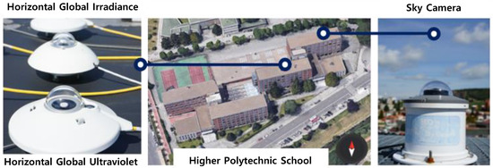
Figure 1. Experimental equipment.

${\mathrm{I}}_{\mathrm{GH}}$, ${\mathrm{I}}_{\mathrm{DH}},$ and ${\mathrm{I}}_{\mathrm{BH}}$ were measured with Hulseflux pyranometers (model SR11: sensitivity of 12.13 µV/(W/m²) and uncertainty of ±1.8%) and a pyrheliometer (model DR01: sensitivity of 10 × 10⁻⁶ V/(W/m²) and uncertainty of ±1.2%), respectively. For direct and diffuse radiation measurements, ${\mathrm{I}}_{\mathrm{DH}}$ and ${\mathrm{I}}_{\mathrm{BH}}$, a GEONICA-SEMS-3000 sun tracker equipped with a shading disc has been used. A Kipp & Zonnen pyranometer (model CUV5: sensitivity of 300–500 µV/(W/m²) and uncertainty of ±5%) was used to determine the ${\mathrm{I}}_{\mathrm{UV}}$ values. The cloud cover was calculated with a commercial SONA201D all-sky camera (Sieltec Canary Islands, Spain). The trigger frequency of the camera was 1 s and its image resolution was 1158 × 1172 pixels, recorded with the RGB color model (8-bit pixels with integer values between 0 and 255 were used). A complete description of the experimental facility and instruments can be found in previous works [14,38,39].

2.2. Statistical Parameters and Estimators

In addition to the experimental measurements (${\mathrm{I}}_{\mathrm{GH}}$, ${\mathrm{I}}_{\mathrm{DH}}$, and ${\mathrm{I}}_{\mathrm{BH}}$, as indicated above), other meteorological variables easily obtained from those values were used. Δ is the sky’s brightness, as shown in Equation (2). It quantifies cloud thickness or aerosol loading.

$$\Delta =\frac{{\mathrm{I}}_{\mathrm{DH}}\ast \mathrm{m}}{{\mathrm{B}}_{\mathrm{sc}}·{\mathsf{\epsilon }}_0}$$

(2)

where ${\mathrm{B}}_{\mathrm{sc}}$ is the extraterrestrial irradiance constant ($=1361.1$W/m² [40]) and m is the relative optical air mass. The sky’s clearness index, $\mathsf{\epsilon },$predicts cloud conditions using the ratio between the diffuse horizontal irradiance and the direct one on the same plane, as shown in Equation (3), where $\mathrm{k}=1.041$ for Z in radians.

$$\mathsf{\epsilon }=\left(\frac{{\mathrm{I}}_{\mathrm{DH}}+\mathrm{I}}{{\mathrm{I}}_{\mathrm{DH}}}+{\mathrm{kZ}}^3\right)/\left(1+{\mathrm{kZ}}^3\right)$$

(3)

The clearness index, ${\mathrm{k}}_{\mathrm{t}}$, obtained with Equation (4), defined as the ratio of the global horizontal irradiance at ground level and the extra-terrestrial global solar irradiance, measures the fraction of the solar radiation transmitted through the atmosphere.

$${\mathrm{k}}_{\mathrm{t}}=\frac{{\mathrm{I}}_{\mathrm{GH}}}{{\mathrm{B}}_{\mathrm{sc}}·{\mathsf{\epsilon }}_0·\cos \mathrm{Z}}$$

(4)

The sky ratio or diffuse fraction, $\mathrm{D}$, as shown in Equation (5), is defined as the ratio of horizontal diffuse irradiance to horizontal global irradiance. It refers to the cloudiness of the sky and/or the turbidity of the atmosphere.

$$\mathrm{D}=\frac{{\mathrm{I}}_{\mathrm{DH}}}{{\mathrm{I}}_{\mathrm{GH}}}$$

(5)

The goodness-of-fit of the models was calculated in terms of $\mathrm{nMBE}(\%)$ (normalized mean bias error) and $\mathrm{nRMSE}(\%)$ (normalized root mean square error). Equations (6) and (7) show the statistical estimators employed in this study.

$$\mathrm{nMBE}(\%)=100\frac{{{\displaystyle \sum }}_{\mathrm{n}}({\mathrm{X}}_{\mathrm{model}}-{\mathrm{X}}_{\mathrm{measured}})}{{{\displaystyle \sum }}_{\mathrm{n}}{\mathrm{X}}_{\mathrm{measured}}}$$

(6)

$$\mathrm{nRMSE}(\%)=100\frac{\sqrt{\frac{{{\displaystyle \sum }}_{\mathrm{n}}{\left({\mathrm{X}}_{\mathrm{model}}-{\mathrm{X}}_{\mathrm{measured}}\right)}^2}{\mathrm{n}}}}{\frac{{{\displaystyle \sum }}_{\mathrm{n}}{\mathrm{X}}_{\mathrm{measured}}}{\mathrm{n}}}$$

(7)

The Pearson correlation coefficient was used to determine the degree of correlation between ${\mathrm{I}}_{\mathrm{UV}}$ and the meteorological variables under study. The Pearson criterion is based on the Pearson correlation coefficient,$\mathrm{r}$. If there is a strong correlation between ${\mathrm{I}}_{\mathrm{UV}}$ and the selected variable, then the Pearson coefficient will be either 1 (direct correlation) or −1 (inverse correlation). However, a Pearson coefficient close to 0 implies a weak or null correlation. The rule of thumb [41] established five r intervals for the correlation: direct (1 ≥ $\left|\mathrm{r}\right|$ ≥ 0.9), strong (0.9 > $\left|\mathrm{r}\right|$ ≥ 0.7), moderate (0.7 > $\left|\mathrm{r}\right|$ ≥ 0.5), weak (0.5 > $\left|\mathrm{r} \right|$ ≥ 0.3), and negligible ($\left|\mathrm{r}\right|$ < 0.3). Figure 2 shows the correlation between all variables considered in the study. The correlation of ${\mathrm{I}}_{\mathrm{UV}}$with the independent meteorological variables is obtained from the last row/column of the correlation matrix shown in Figure 2. The influence of these variables on ${\mathrm{I}}_{\mathrm{UV}}$ can also be seen graphically in Figure 3, where the input variables have been ordered according to the correlation with ${\mathrm{I}}_{\mathrm{UV}}$.

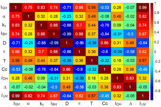
Figure 2. The Pearson correlation coefficient matrix of all meteorological variables considered in this study.

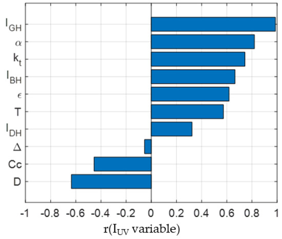
Figure 3. The Pearson correlation coefficient, r(I_UV, variable), between ${\mathrm{I}}_{\mathrm{UV}}$ and the meteorological variables considered in the study.

The meteorological variables with $\mathrm{r}\left({\mathrm{I}}_{\mathrm{UV}},\mathrm{variable}\right)<0.4$ were discarded as inputs for the models, after which only the variables included in Table 1 were considered.

Table 1. Selection of meteorological variables to be considered, according to the Pearson correlation coefficient r(I_UV, variable).

Variable:	IGH	α	kt	IBH	D	ε	T	Cc
r(IUV, variable):	0.99	0.82	0.74	0.67	−0.64	0.62	0.57	−0.45

As Figure 3 shows, ${\mathrm{I}}_{\mathrm{GH}}$ has the strongest correlation with ${\mathrm{I}}_{\mathrm{UV}}$, followed by the solar altitude angle, $\mathsf{\alpha }$, and the clearness index, ${\mathrm{k}}_{\mathrm{t}}$. Only $\mathrm{D}$and $\mathrm{Cc}$presented weak inverse correlation with ${\mathrm{I}}_{\mathrm{UV}}$. The results were coherent with those in the literature review.

3. Artificial Neural Network Models

A topology consisting of an input layer, a hidden layer, and an output layer was considered for the ANN, and the Levenberg–Marquardt algorithm was used to adjust both the weights and the bias of the network, in accordance with Equation (8). The transfer function in the hidden layer, ${\mathrm{f}}_1$, was sigmoidal, and f₂ in the output layer was a linear function. ${\mathrm{W}}_1$ and ${\mathrm{b}}_1$ were the weights and biases of the hidden layer, and ${\mathrm{W}}_2$ and ${\mathrm{b}}_2$ were the weights and biases of the output layer, respectively.

$${\mathrm{I}}_{\mathrm{UV}}={\mathrm{f}}_2\left({\mathrm{W}}_2{\ast \mathrm{f}}_1\left({\mathrm{W}}_1\ast \mathrm{Inputs}+{\mathrm{b}}_1\right)+{\mathrm{b}}_2\right)$$

(8)

All the meteorological variables indicated in Table 1 may be used to develop ANN-based models. As indicated above, ${\mathrm{I}}_{\mathrm{GH}}$ is the variable with the greatest influence on ${\mathrm{I}}_{\mathrm{UV}}$. The Pearson correlation coefficient is 0.99, as shown in Figure 2. Therefore, ${\mathrm{I}}_{\mathrm{GH}}$ must be included as a first input of the model. However, some of the variables are correlated between each other and their inclusion together in the ANN model increased the complexity of the model without significantly improving accuracy, both for the $\mathrm{nRMSE}$ and the $\mathrm{nMBE}$ values. As can be seen in Table 2, the Pearson coefficient $\mathrm{r}\left({\mathrm{I}}_{\mathrm{GH}}\mathrm{variable}\right)$highlighted a high correlation between ${\mathrm{I}}_{\mathrm{GH}}$ and ${\mathrm{k}}_{\mathrm{t}}$. On the other hand, as can be observed in Figure 2, a high correlation exits between${\mathrm{I}}_{\mathrm{BH}}$, and $\mathrm{D}$. To determine the optimal neural network, the goodness of fit of the models obtained with the combination of inputs shown in Table 3 was analyzed, using the previously defined indicators, $\mathrm{nRMSE},$ and $\mathrm{nMBE}$. In each combination, one of the variables was eliminated or substituted. For the analysis, the experimental data set was divided into three groups: 70% was used as a training set, 15% as a validation set, and the remaining 15% was used to test the model. The three (training, validation and test) data sets were the same in all the models that were developed.

Table 2. The Pearson correlation coefficient $\mathrm{r}\left({\mathrm{I}}_{\mathrm{GH}},\mathrm{variable}\right)$ for detecting redundant information.

Variable:	${\mathbf{k}}_{\mathbf{t}}$	α	${\mathbf{I}}_{\mathbf{B}\mathbf{H}}$	$\mathbf{D}$	ε	$\mathbf{T}$	$\mathbf{C}\mathbf{c}$
${\mathrm{r}}_{\left({\mathrm{I}}_{\mathrm{GH}},\mathrm{Variable}\right)}$:	0.83	0.75	0.74	−0.71	0.66	0.56	−0.53

Table 3. Results of ${\mathrm{I}}_{\mathrm{UV}}$ ANN models.

Model Number & Variables		Training			Test
#	Variables	$\mathbf{n}\mathbf{R}\mathbf{M}\mathbf{S}\mathbf{E} \left(\mathbf{\%}\right)$	$\mathbf{n}\mathbf{M}\mathbf{B}\mathbf{E} \left(\mathbf{\%}\right)$	${\mathbf{R}}^2$ (%)	$\mathbf{n}\mathbf{R}\mathbf{M}\mathbf{S}\mathbf{E} \left(\mathbf{\%}\right)$	$\mathbf{n}\mathbf{M}\mathbf{B}\mathbf{E} \left(\mathbf{\%}\right)$	${\mathbf{R}}^2$ (%)
1	$I_{GH}$, $k_t$, α, $I_{BH}$, $D$, ε,  $T$, $Cc$	3.82	0.00	99.68%	3.77	−0.01	99.69%
2	$I_{GH}$, α, $I_{BH}$, $D$, ε, $T$, $Cc$	3.87	0.00	99.67%	3.83	−0.01	99.68%
3	$I_{GH}$, $I_{BH}$, $D$, ε, $T$, $Cc$	4.26	−0.01	99.60%	4.21	−0.01	99.62%
4	$I_{GH}$, α, $D$, ε,  $T$, $Cc$	3.89	0.00	99.67%	3.86	−0.02	99.68%
5	$I_{GH}$, α, ε, $T$, $Cc$	3.91	−0.02	99.66%	3.88	−0.03	99.67%
6	$I_{GH}$, α, $T$, $Cc$	4.04	0.00	99.64%	4.01	−0.01	99.65%
7	$I_{GH}$, α, ε, $Cc$	4.15	0.00	99.62%	4.09	0.00	99.64%
8	$I_{GH}$, α, $T$	4.85	0.00	99.48%	4.82	0.04	99.49%
9	$I_{GH}$, α, $Cc$	4.30	0.00	99.59%	4.24	0.00	99.61%
10	$I_{GH}$, α, $\mathsf{\epsilon }$	4.71	−0.01	99.51%	4.67	0.02	99.53%
11	$I_{GH}$, α	5.13	0.01	99.42%	5.09	0.07	99.44%
12	$I_{GH}$	10.30	0.00	97.66%	10.29	0.19	97.70%
13	$k_t$, α, $Cc$	4.36	0.00	99.58%	4.34	0.02	99.59%
14	$k_t$, α	5.13	0.00	99.42%	5.10	0.05	99.44%
15	$k_t$	39.72	−0.05	65.26%	40.08	0.58	65.14%
16	$I_{BH}$, α, $Cc$	8.70	−0.01	98.33%	8.55	0.08	98.41%
17	$I_{BH}$, α	11.94	0.00	96.86%	12.03	−0.02	96.86%
18	$I_{BH}$	45.45	0.00	54.50%	46.05	0.45	53.98%

Table 3 shows the 18 ANN models developed with the $\mathrm{nRMSE},$ $\mathrm{nMBE}$, and the corresponding ${\mathrm{R}}^2$ values obtained for the data used in both the training and in the test models.

The results shown in Table 3 confirmed that the inclusion of meteorological variables with a high Pearson correlation coefficient in no way improved the accuracy of the ANN. On the one hand, considering ${\mathrm{I}}_{\mathrm{GH}}$, α, ε, $\mathrm{T}$, $\mathrm{Cc}$, ANN model number 5 might be more appropriate than models 1 to 4 listed in Table 3. On the other hand, eliminating solar height had a negative influence on the values of the statistics under analysis. Therefore, solar height was left as an independent variable in the models. Likewise, worse results were observed after removing cloud cover and leaving temperature. Based on the above, the model to be used was model number 9, from Table 3, as that model presented a reduced number of inputs (${\mathrm{I}}_{\mathrm{GH}}$, α, $\mathrm{Cc}$) and yielded adequate $\mathrm{nRMSE}$ and $\mathrm{nMBE}$ values. In addition, it was observed that model 9, which uses ${\mathrm{I}}_{\mathrm{GH}}$, yielded a somewhat lower $\mathrm{nRMSE}$ than model 13, obtained using ${\mathrm{k}}_{\mathrm{t}}$ instead of ${\mathrm{I}}_{\mathrm{GH}}$ and with the two other above-mentioned variables (α, $\mathrm{Cc})$. However, both models could be used, as they yielded similar results. On the other hand, significantly worse statistics were observed when using ${\mathrm{I}}_{\mathrm{BH}}$ instead of ${\mathrm{I}}_{\mathrm{GH}}$ with the two previously mentioned variables (α, $\mathrm{Cc}$). It can be seen that the selected model (model 9) presented an ${\mathrm{R}}^2$ of 99.59% with the training dataset, and of 99.61% with the test dataset, and similar values were obtained with the model that used ${\mathrm{k}}_{\mathrm{t}}$ instead of ${\mathrm{I}}_{\mathrm{GH}}$.

Figure 4 shows the relationship between ${\mathrm{I}}_{\mathrm{UV}}$ and${\mathrm{I}}_{\mathrm{GH}}$ based on the data considered in this study. Both the training and the test datasets showed similar distributions.

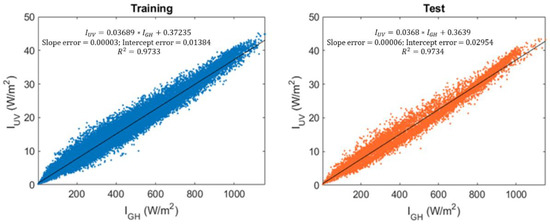
Figure 4. Ultraviolet irradiance, ${\mathrm{I}}_{\mathrm{UV},}$ vs. global horizontal irradiance, ${\mathrm{I}}_{\mathrm{GH}}$.

Figure 5 also shows the relationship between solar height and ultraviolet radiation for both the training and test datasets. These figures are included because solar height will be a variable that will be part of the selected models, as can be seen in Table 3, while Figure 6 represents the ultraviolet radiation vs. cloud cover for both datasets.

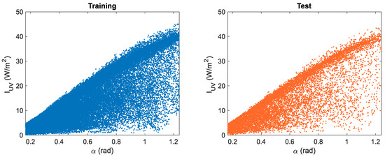
Figure 5. Ultraviolet irradiance, ${\mathrm{I}}_{\mathrm{UV}}$, vs. solar altitude, α.

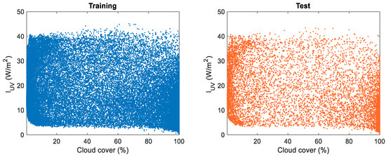
Figure 6. Ultraviolet irradiance, ${\mathrm{I}}_{\mathrm{UV}}$, vs. cloud cover, $\mathrm{Cc}$.

Figure 7 shows the values predicted with ANN model number 9, where the “Output” corresponds to the neural network outputs and “Target” to the experimental values for both training and test dataset results.

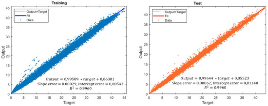
Figure 7. Results of${\mathrm{I}}_{\mathrm{UV}}=\mathrm{f}\left({\mathrm{I}}_{\mathrm{GH}},\mathsf{\alpha },\mathrm{Cc}\right)$, using ANN model 9.

4. Regression Models

Having determined the ANN-based models, a regression fit was performed with the same selected variables (${\mathrm{I}}_{\mathrm{GH}}$, α, and $\mathrm{Cc}$) analyzing first and second-order models. A similar study was also performed with (${\mathrm{k}}_{\mathrm{t}}$, α, and $\mathrm{Cc}$). The models were fitted with 85% of the data to generate the regression models, and the remaining 15% of the data were used to test the models. The data used for fitting and testing the regression models were the same as those used for the ANN models. It should be noted that when using ${\mathrm{I}}_{\mathrm{BH}}$ instead of ${\mathrm{I}}_{\mathrm{GH}}$ or ${\mathrm{k}}_{\mathrm{t}}$, the accuracy of the models worsened significantly, which could be expected a priori in view of the correlation matrix shown in Figure 2. Therefore, these models were not included in the present study.

From the data shown in Figure 4 an approximately linear relationship between ${\mathrm{I}}_{\mathrm{UV}}$ and ${\mathrm{I}}_{\mathrm{GH}}$ can be deduced after fitting a first-order model as a function of ${\mathrm{I}}_{\mathrm{GH}}$, ${\mathrm{I}}_{\mathrm{UV}}=0.3676+0.0369·{\mathrm{I}}_{\mathrm{GH}}$. It could therefore be considered, as an approximate value, that ${\mathrm{I}}_{\mathrm{UV}}$ was 3.7% of ${\mathrm{I}}_{\mathrm{GH}}$, for the data analyzed within the study period and in the locality of Burgos, Spain. The results with the linear model${\mathrm{R}}^2=97.32\%$, $\mathrm{RSME}=11.02\%$, and $\mathrm{nMBE}=0.00\%$ were worse than those obtained with more complex models, which included a larger number of variables but had the advantage of simplicity.

The following linear regression models given by Equation (9) can be considered as a first option, in the case of preferring greater accuracy, than the linear model with ${\mathrm{I}}_{\mathrm{GH}}$ without using ANNs:

$${\mathrm{I}}_{\mathrm{UV}}={\mathrm{b}}_0+{{\displaystyle \sum }}_{\mathrm{j}=1}^3{\mathrm{b}}_{\mathrm{j}}{ \ast \mathrm{x}}_{\mathrm{j}}$$

(9)

Although this means including more independent variables in the model. The use of a second-order regression model, such as the one shown in Equation (10), could also be considered, should greater precision be needed:

$${\mathrm{I}}_{\mathrm{UV}}={\mathrm{b}}_0+{{\displaystyle \sum }}_{\mathrm{j}=1}^3{\mathrm{b}}_{\mathrm{j}}{ \ast \mathrm{x}}_{\mathrm{j}}+{{\displaystyle \sum }}_{\mathrm{j}=1}^3{\mathrm{b}}_{\mathrm{jj}}{ \ast \mathrm{x}}_{\mathrm{j}}^2+{{\displaystyle \sum }}_{\begin{array}{c}\mathrm{k}>\mathrm{j}\\ \mathrm{j}=1,2\end{array}}^3{\mathrm{b}}_{\mathrm{jk}}{ \ast \mathrm{x}}_{\mathrm{j}}{ \ast \mathrm{x}}_{\mathrm{k}}$$

(10)

Equations (9) and (10) show the first-order and the second-order models to be fitted to the ultraviolet irradiance model, considering${\mathrm{x}}_1={\mathrm{I}}_{\mathrm{GH}},{\mathrm{x}}_2={\mathsf{\alpha }\mathrm{and}\mathrm{x}}_3=\mathrm{Cc}$ both in the first-order and the second-order models. Equation (11) shows the first-order regression model fitted with the above three variables, and Equation (12) also shows the linear regression model fitted only for ${\mathrm{I}}_{\mathrm{GH}}$ and solar altitude, i.e., eliminating cloud cover from the linear-regression model.

$$\begin{array}{l}{I}_{UV}\mathbf{=}\mathbf{-}\mathbf{1.9243}\mathbf{+}\mathbf{0.0323}\mathbf{·}{I}_{GH}\mathbf{+}\mathbf{6.5892}\mathbf{\ast }\mathsf{\alpha }\mathbf{+}\mathbf{0.0035}\mathbf{·}Cc \hfill \\ \left[R_{\mathbf{Training}}^{\mathbf{2}}\mathbf{=}\mathbf{98.83}\mathbf{\%}\mathbf{,} {\mathbf{nRMSE}}_{\mathbf{Training}}\mathbf{=}\mathbf{7.29}\mathbf{\%}\mathbf{,} {\mathbf{nMBE}}_{\mathbf{Training}}\mathbf{=}\mathbf{0.00}\mathbf{\%}\right] \hfill \\ \left[{\mathrm{R}}_{\mathrm{Test}}^2=98.82\%,{\mathrm{nRMSE}}_{\mathrm{Test}}=7.36\%,{\mathrm{nMBE}}_{\mathrm{Test}}=0.11\%\right]\hfill \end{array}$$

(11)

$$\begin{array}{l}{\mathrm{I}}_{\mathrm{UV}}=-1.7224+0.0317·{\mathrm{I}}_{\mathrm{GH}}+6.9531·\mathsf{\alpha }\hfill \\ \left[{\mathrm{R}}_{\mathrm{Training}}^2=98.82\%,{\mathrm{nRMSE}}_{\mathrm{Training}}=7.32\%,{\mathrm{nMBE}}_{\mathrm{Training}}=0.00\%\right]\hfill \\ \left[{\mathrm{R}}_{\mathrm{Test}}^2=98.81\%,{\mathrm{nRMSE}}_{\mathrm{Test}}=7.39\%,{\mathrm{nMBE}}_{\mathrm{Test}}=0.11\%\right]\hfill \end{array}$$

(12)

Equation (13) shows the second-order model, with the three independent variables selected for ANN model 9, fitted to the data that are studied in this work.

$$\begin{gathered} \begin{array}{l}{\mathrm{I}}_{\mathrm{UV}}=-1.8212+0.0167·{\mathrm{I}}_{\mathrm{GH}}+19.0462·\mathsf{\alpha }+0.0126·\mathrm{Cc}-9.29·{10}^{-6}·{\mathrm{I}}_{\mathrm{GH}}^2+0.0188·{\mathrm{I}}_{\mathrm{GH}}·\mathsf{\alpha }+8.80·{10}^{-5} \\ ·{\mathrm{I}}_{\mathrm{GH}}·\mathrm{Cc}-7.2559·{\mathsf{\alpha }}^2-0.0958·\mathsf{\alpha }·\mathrm{Cc}-6.59·{10}^{-5}·{\mathrm{Cc}}^2\hfill \\ [{\mathrm{R}}_{\mathrm{Training}}^2=99.43\%,{\mathrm{nRMSE}}_{\mathrm{Training}}=5.06\%,{\mathrm{nMBE}}_{\mathrm{Training}}=0.00\%]\hfill \\ [{\mathrm{R}}_{\mathrm{Test}}^2=99.45\%,{\mathrm{nRMSE}}_{\mathrm{Test}}=5.02\%,{\mathrm{nMBE}}_{\mathrm{Test}}=0.06\%]\hfill \end{array} \end{gathered}$$

(13)

A simpler model is shown in Equation (14), in which cloud cover is removed as an independent variable, which may be useful if cloud-cover data are unavailable.

$$\begin{array}{l}{\mathrm{I}}_{\mathrm{UV}}=-1.1625+0.0238·{\mathrm{I}}_{\mathrm{GH}}+10.2243·\mathsf{\alpha }-1.27·{10}^{-5}·{\mathrm{I}}_{\mathrm{GH}}^2+0.0253·{\mathrm{I}}_{\mathrm{GH}}·\mathsf{\alpha }-8.8361·{\mathsf{\alpha }}^2\hfill \\ [{\mathrm{R}}_{\mathrm{Training}}^2=99.30\%,{\mathrm{nRMSE}}_{\mathrm{Training}}=5.63\%,{\mathrm{nMBE}}_{\mathrm{Training}}=0.00\%]\hfill \\ [{\mathrm{R}}_{\mathrm{Test}}^2=99.32\%,{\mathrm{nRMSE}}_{\mathrm{Test}}=5.60\%,{\mathrm{nMBE}}_{\mathrm{Test}}=0.07\%]\hfill \end{array}$$

(14)

A study was also conducted on the use of ${\mathrm{k}}_{\mathrm{t}}$ instead of ${\mathrm{I}}_{\mathrm{GH}}$. In this case, the values are shown below in Equations (15)–(18).

$${\mathrm{I}}_{\mathrm{UV}}=-11.3956+22.8218·{\mathrm{k}}_{\mathrm{t}}+24.3899·+0.0021·\mathrm{Cc}$$

(15)

$$\begin{array}{cc}& \left[{\mathbf{R}}_{\mathbf{Training}}^{\mathbf{2}}\mathbf{=}\mathbf{93.18}\mathbf{\%}\mathbf{,}{\mathbf{nRMSE}}_{\mathbf{Training}}\mathbf{=}\mathbf{17.57}\mathbf{\%}\mathbf{,}{\mathbf{nMBE}}_{\mathbf{Training}}=\mathbf{0.00}\mathbf{\%}\right]\hfill \\ & \left[{\mathbf{R}}_{\mathbf{Test}}^{\mathbf{2}}\mathbf{=}\mathbf{93.01}\mathbf{\%},{\mathbf{nRMSE}}_{\mathbf{Test}}\mathbf{=}\mathbf{17.95}\mathbf{\%}\mathbf{,}{\mathbf{nMBE}}_{\mathbf{Test}}\mathbf{=}\mathbf{0.11}\mathbf{\%}\right]\hfill \\ & {\mathrm{I}}_{\mathrm{UV}}=-11.1581+22.5424·{\mathrm{k}}_{\mathrm{t}}+24.4465·\mathsf{\alpha }\hfill \end{array}$$

(16)

$$\begin{array}{cc}& \left[{\mathbf{R}}_{\mathbf{Training}}^{\mathbf{2}}\mathbf{=}\mathbf{93.18}\mathbf{\%}\mathbf{,}\mathbf{n}\mathbf{R}\mathbf{M}\mathbf{S}{\mathbf{E}}_{\mathbf{Training}}\mathbf{=}\mathbf{17.57}\mathbf{\%}\mathbf{,}\mathbf{n}\mathbf{M}\mathbf{B}{\mathbf{E}}_{\mathbf{Training}}\mathbf{=}\mathbf{0.00}\mathbf{\%}\right]\hfill \\ & \left[{\mathbf{R}}_{\mathbf{Test}}^{\mathbf{2}}\mathbf{=}\mathbf{93.01}\mathbf{\%}\mathbf{,}{\mathbf{nRMSE}}_{\mathbf{Test}}\mathbf{=}\mathbf{17.95}\mathbf{\%}\mathbf{,}\mathbf{n}\mathbf{M}\mathbf{B}{\mathbf{E}}_{\mathbf{Test}}\mathbf{=}\mathbf{0.11}\mathbf{\%}\right]\hfill \\ & {\mathbf{I}}_{\mathbf{UV}}\mathbf{=}\mathbf{-}\mathbf{0.3544}\mathbf{+}\mathbf{2.0833}\mathbf{·}{\mathbf{k}}_{\mathbf{t}}\mathbf{+}\mathbf{14.0893}\mathbf{·}\mathbf{\alpha }\mathbf{-}\mathbf{0.0165}\mathbf{·}\mathbf{C}\mathbf{c}\mathbf{-}\mathbf{9.0813}\mathbf{·}{\mathbf{k}}_{\mathbf{t}}^{\mathbf{2}}\mathbf{+}\mathbf{40.7916}\mathbf{·}{\mathbf{k}}_{\mathbf{t}}\mathbf{·}\mathbf{\alpha }\hfill \\ & \hfill \mathbf{+}\mathbf{0.0405}\mathbf{·}{\mathbf{k}}_{\mathbf{t}}\mathbf{·}\mathbf{C}\mathbf{c}\mathbf{-}\mathbf{7.9650}\mathbf{·}{\mathbf{\alpha }}^{\mathbf{2}}\mathbf{-}\mathbf{0.0170}\mathbf{·}\mathbf{\alpha }\mathbf{·}\mathbf{C}\mathbf{c}\mathbf{-}\mathbf{8.83}\mathbf{·}\mathbf{1}{\mathbf{0}}^{\mathbf{-}\mathbf{5}}\mathbf{·}\mathbf{C}{\mathbf{c}}^{\mathbf{2}}\hfill \\ & \left[{\mathbf{R}}_{\mathbf{Training}}^{\mathbf{2}}\mathbf{=}\mathbf{99.39}\mathbf{\%}\mathbf{,}\mathbf{n}\mathbf{R}\mathbf{M}\mathbf{S}{\mathbf{E}}_{\mathbf{Training}}\mathbf{=}\mathbf{5.26}\mathbf{\%}\mathbf{,}\mathbf{n}\mathbf{M}\mathbf{B}{\mathbf{E}}_{\mathbf{Training}}\mathbf{=}\mathbf{0.00}\mathbf{\%}\right]\hfill \\ & \left[{\mathbf{R}}_{\mathbf{Test}}^{\mathbf{2}}\mathbf{=}\mathbf{99.40}\mathbf{\%}\mathbf{,}\mathbf{n}\mathbf{R}\mathbf{M}\mathbf{S}{\mathbf{E}}_{\mathbf{Test}}\mathbf{=}\mathbf{5.24}\mathbf{\%}\mathbf{,}\mathbf{n}\mathbf{M}\mathbf{B}{\mathbf{E}}_{\mathbf{Test}}\mathbf{=}\mathbf{0.08}\mathbf{\%}\right]\hfill \end{array}$$

(17)

Analogously to ${\mathrm{I}}_{\mathrm{GH}}$, the model in Equation (17), in which cloud cover as an independent variable is removed, is useful if the cloud-cover data are unavailable.

$$\begin{array}{cc}& {\mathbf{I}}_{\mathbf{UV}}\mathbf{=}\mathbf{-}\mathbf{2.7058}\mathbf{+}\mathbf{7.3586}\mathbf{·}{\mathbf{k}}_{\mathbf{t}}\mathbf{+}\mathbf{11.4945}·\mathbf{\alpha }\mathbf{-}\mathbf{10.8880}\mathbf{·}\mathbf{+}\mathbf{42.6023}\mathbf{·}{\mathbf{k}}_{\mathbf{t}}\mathbf{·}\mathbf{\alpha }\mathbf{-}\mathbf{7.7515}\hfill \\ & \hspace{1em}\hspace{1em}\hspace{1em}\hspace{1em}\hspace{1em}·{\mathsf{\alpha }}^2\hfill \\ & \left[{\mathbf{R}}_{\mathbf{Training}}^{\mathbf{2}}\mathbf{=}\mathbf{99.30}\mathbf{\%},{\mathbf{nRMSE}}_{\mathbf{Training}}\mathbf{=}\mathbf{5.63}\mathbf{\%}\mathbf{,}\mathbf{n}\mathbf{M}\mathbf{B}{\mathbf{E}}_{\mathbf{Training}}\mathbf{=}\mathbf{0.00}\mathbf{\%}\right]\hfill \\ & \left[{\mathrm{R}}_{\mathrm{Test}}^2=99.32\%,{\mathrm{nRMSE}}_{\mathrm{Test}}=5.62\%,{\mathrm{nMBE}}_{\mathrm{Test}}=0.08\%\right]\hfill \end{array}$$

(18)

It can be observed that when quadratic terms are included in the regression models, the models containing ${\mathrm{k}}_{\mathrm{t}}$ instead of ${\mathrm{I}}_{\mathrm{GH}}$ led to similar results, with the models containing ${\mathrm{I}}_{\mathrm{GH}}$ yielding somewhat better results. Therefore, in the case of using a second-order model, it may be preferable to use ${\mathrm{k}}_{\mathrm{t}}$ in the formulation, as it gives an idea of the clearness of the sky, and the results are similar to using ${\mathrm{I}}_{\mathrm{GH}}$. The same is not true when using linear models, where the accuracy of considering ${\mathrm{k}}_{\mathrm{t}}$ in the formulation worsens significantly, as can be seen when comparing Equations (15) and (16) with (11) and (12), which correspond to the first order models for ${\mathrm{k}}_{\mathrm{t}}$and ${\mathrm{I}}_{\mathrm{GH}}$, respectively. Therefore, the use of first-order models makes it preferable to introduce ${\mathrm{I}}_{\mathrm{GH}}$ in the formulation, as the models with ${\mathrm{k}}_{\mathrm{t}}$ yielded less accurate results.

Figure 8, Figure 9 and Figure 10 show the response surfaces obtained with the second-order regression models shown in Equations (13) and (17), which correspond to the second-order regression models developed for ${\mathrm{I}}_{\mathrm{GH}}$, α, and cloud cover and for ${\mathrm{k}}_{\mathrm{t}}$, α, and cloud cover, respectively.

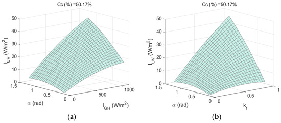
Figure 8. (a) ${\mathrm{I}}_{\mathrm{UV}}\mathrm{vs}.{\left(\mathsf{\alpha },{\mathrm{I}}_{\mathrm{GH}}\right)|}_{\mathrm{Cc}=\mathrm{constant}}$ and (b) ${\mathrm{I}}_{\mathrm{UV}}\mathrm{vs}.{\left(\mathsf{\alpha },{\mathrm{k}}_{\mathrm{t}}\right)|}_{\mathrm{Cc}=\mathrm{constant}}$.

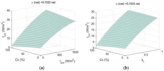
Figure 9. (a) ${\mathrm{I}}_{\mathrm{UV}}\mathrm{vs}.{\left(\mathrm{Cc},{\mathrm{I}}_{\mathrm{GH}}\right)|}_{=\mathrm{constant}}$ and (b) ${\mathrm{I}}_{\mathrm{UV}}\mathrm{vs}.{\left(\mathrm{Cc},{\mathrm{k}}_{\mathrm{t}}\right)|}_{=\mathrm{constant}}$.

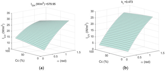
Figure 10. (a) ${\mathrm{I}}_{\mathrm{UV}}\mathrm{vs}.{\left(\mathrm{Cc},\mathsf{\alpha }\right)|}_{{\mathrm{I}}_{\mathrm{GH}}=\mathrm{constant}}$ and (b) ${\mathrm{I}}_{\mathrm{UV}}\mathrm{vs}.{\left(\mathrm{Cc},\mathsf{\alpha }\right)|}_{{\mathrm{k}}_{\mathrm{t}}=\mathrm{constant}}$.

5. Conclusions

In the present work, different models have been analyzed for the determination of horizontal ultraviolet irradiance based on meteorological and radiative variables collected in Burgos (Spain), using supervised ANNs and regression models.

The ANN-based models presented higher accuracy in their predictions of horizontal ultraviolet irradiance than the regression-based models. Specifically, in the case of the selected model, which included ${\mathrm{I}}_{\mathrm{GH}}$, α, and $\mathrm{Cc}$ as independent variables, the datasets used to train the neural network and the test data yielded $\mathrm{nRMSE}$ readings of 4.30% and 4.24%, respectively. This ANN-based model was more accurate than the one obtained with the second-order regression model, which used the same variables and yielded $\mathrm{nRMSE}$ readings of 5.06% and 5.02% with the training and the test datasets, respectively.

It has also been observed that when quadratic terms were included in the regression models, the models containing ${\mathrm{k}}_{\mathrm{t}}$ rather than ${\mathrm{I}}_{\mathrm{GH}}$ yielded similar results, while the models containing ${\mathrm{I}}_{\mathrm{GH}}$ were somewhat better. In the case of using the neural network with ${\mathrm{k}}_{\mathrm{t}}$, α and $\mathrm{Cc}$ as independent variables, $\mathrm{nRMSE}$ readings of 4.36% and 4.34% were obtained with the training and the test datasets, respectively. Analogously to the case of ${\mathrm{I}}_{\mathrm{GH}}$, the ANN-based model for ${\mathrm{k}}_{\mathrm{t}}$ was more accurate than the model obtained for ${\mathrm{k}}_{\mathrm{t}}$ with a second-order regression fit using the same variables yielding $\mathrm{nRMSE}$ readings of 5.26% and 5.24% for the training and the test datasets, respectively.

It may therefore be preferable to use ${\mathrm{k}}_{\mathrm{t}}$ in the formulation in the case of using a second-order model, as it gives an idea of the clearness of the sky and the results are similar to those obtained when using ${\mathrm{I}}_{\mathrm{GH}}$. The same could not be said when using linear models, with which the accuracy when considering ${\mathrm{k}}_{\mathrm{t}}$ in the formulation worsened significantly.

In the case that cloud cover measurements are not available, models 11 and 14 in Table 3, which have only two independent variables ($\mathsf{\alpha }$ and ${\mathrm{I}}_{\mathrm{GH}}$) and ($\mathsf{\alpha }$ and ${\mathrm{k}}_{\mathrm{t}}$), respectively, and which can be easily measured at most stations, present results with high $\mathrm{nRMSE}$ accuracy (5.13% in both cases); they can be useful for predicting ultraviolet radiation.The effectiveness of the above methods for modeling horizontal ultraviolet irradiance has been demonstrated, using a reduced number of variables, with the data analyzed in the present study.

References

- Alados-Arboledas, L.; Alados, I.; Foyo-Moreno, I.; Olmo, F.J.; Alcántara, A. The Influence of Clouds on Surface UV Erythemal Irradiance. Atmos. Res. 2003, 66, 273–290. [Google Scholar] [CrossRef]
- Hu, B.; Wang, Y.; Liu, G. Variation Characteristics of Ultraviolet Radiation Derived from Measurement and Reconstruction in Beijing, China. Tellus Ser. B Chem. Phys. Meteorol. 2010, 62, 100–108. [Google Scholar] [CrossRef]
- Murillo, W.; Cañada, J.; Pedrós, G. Correlation between Global Ultraviolet (290–385 nm) and Global Irradiation in Valencia and Cordoba (Spain). Renew. Energy 2003, 28, 409–418. [Google Scholar] [CrossRef]
- Human, S.; Bajic, V. Modelling Ultraviolet Irradiance in South Africa. Radiat. Prot. Dosim. 2000, 91, 181–183. [Google Scholar] [CrossRef]
- Modenese, A.; Gobba, F.; Paolucci, V.; John, S.M.; Sartorelli, P.; Wittlich, M. Occupational Solar UV Exposure in Construction Workers in Italy: Results of a One-Month Monitoring with Personal Dosimeters. In Proceedings of the 2020 IEEE International Conference on Environment and Electrical Engineering and 2020 IEEE Industrial and Commercial Power Systems Europe (EEEIC/I&CPS Europe), Madrid, Spain, 9–12 June 2020; pp. 6–10. [Google Scholar] [CrossRef]
- Ahmed, A.A.M.; Ahmed, M.H.; Saha, S.K.; Ahmed, O.; Sutradhar, A. Optimization Algorithms as Training Approach with Hybrid Deep Learning Methods to Develop an Ultraviolet Index Forecasting Model. Stoch. Environ. Res. Risk Assess. 2022, 36, 3011–3039. [Google Scholar] [CrossRef]
- Al-Aruri, S.D. The Empirical Relationship between Global Radiation and Global Ultraviolet (0.290–0.385) μm Solar Radiation Components. Sol. Energy 1990, 45, 61–64. [Google Scholar] [CrossRef]
- Modenese, A.; Bisegna, F.; Borra, M.; Burattini, C.; Gugliermetti, L.; Filon, F.L.; Militello, A.; Toffanin, P.; Gobba, F. Occupational Exposure to Solar UV Radiation in a Group of Dock-Workers in North-East Italy. In Proceedings of the 2020 IEEE International Conference on Environment and Electrical Engineering and 2020 IEEE Industrial and Commercial Power Systems Europe (EEEIC/I&CPS Europe), Madrid, Spain, 9–12 June 2020; pp. 16–21. [Google Scholar] [CrossRef]
- Lamy, K.; Portafaix, T.; Brogniez, C.; Godin-Beekmann, S.; Bencherif, H.; Morel, B.; Pazmino, A.; Metzger, J.M.; Auriol, F.; Deroo, C.; et al. Ultraviolet Radiation Modelling from Ground-Based and Satellite Measurements on Reunion Island, Southern Tropics. Atmos. Chem. Phys. 2018, 18, 227–246. [Google Scholar] [CrossRef]
- Serrano, M.A.; Cañada, J.; Moreno, J.C.; Gurrea, G. Solar Ultraviolet Doses and Vitamin D in a Northern Mid-Latitude. Sci. Total Environ. 2017, 574, 744–750. [Google Scholar] [CrossRef]
- Leal, S.S.; Tíba, C.; Piacentini, R. Daily UV Radiation Modeling with the Usage of Statistical Correlations and Artificial Neural Networks. Renew. Energy 2011, 36, 3337–3344. [Google Scholar] [CrossRef]
- Dahr, F.E.; Bah, A.; Ghennioui, A. Estimation of Ultraviolet Solar Irradiation of Semi-Arid Area—Case of Benguerir. In Proceedings of the 2020 International Conference on Electrical and Information Technologies (ICEIT), Rabat, Morocco, 4–7 March 2020; pp. 1–5. [Google Scholar] [CrossRef]
- Zhang, X.; Hu, B.; Wang, Y.; Lu, J. Reconstruction of Daily Ultraviolet Radiation for Nine Observation Stations in China. J. Atmos. Chem. 2014, 71, 303–319. [Google Scholar] [CrossRef]
- García-Rodríguez, S.; García, I.; García-Rodríguez, A.; Díez-Mediavilla, M.; Alonso-Tristán, C. Solar Ultraviolet Irradiance Characterization under All Sky Conditions in Burgos, Spain. Appl. Sci. 2022, 12, 10407. [Google Scholar] [CrossRef]
- Foyo-Moreno, I.; Alados, I.; Olmo, F.J.; Alados-Arboledas, L. The Influence of Cloudiness on UV Global Irradiance (295–385 Nm). Agric. For. Meteorol. 2003, 120, 101–111. [Google Scholar] [CrossRef]
- Foyo-Moreno, I.; Vida, J.; Alados-Arboledas, L. Ground Based Ultraviolet (290–385 Nm) and Broadband Solar Radiation Measurements in South-Eastern Spain. Int. J. Climatol. 1998, 18, 1389–1400. [Google Scholar] [CrossRef]
- Foyo-Moreno, I.; Vida, J.; Alados-Arboledas, L. A Simple All Weather Model to Estimate Ultraviolet Solar Radiation (290–385 Nm). J. Appl. Meteorol. 1999, 38, 1020–1026. [Google Scholar] [CrossRef]
- Bilbao, J.; Mateos, D.; de Miguel, A. Analysis and Cloudiness Influence on UV Total Irradiation. Int. J. Climatol. 2011, 31, 451–460. [Google Scholar] [CrossRef]
- Barbero, F.J.; López, G.; Batlles, F.J. Determination of Daily Solar Ultraviolet Radiation Using Statistical Models and Artificial Neural Networks. Ann. Geophys. 2006, 24, 2105–2114. [Google Scholar] [CrossRef]
- Jacovides, C.P.; Tymvios, F.S.; Boland, J.; Tsitouri, M. Artificial Neural Network Models for Estimating Daily Solar Global UV, PAR and Broadband Radiant Fluxes in an Eastern Mediterranean Site. Atmos. Res. 2015, 152, 138–145. [Google Scholar] [CrossRef]
- Wang, L.; Gong, W.; Luo, M.; Wang, W.; Hu, B.; Zhang, M. Comparison of Different UV Models for Cloud Effect Study. Energy 2015, 80, 695–705. [Google Scholar] [CrossRef]
- Wang, L.; Gong, W.; Li, J.; Ma, Y.; Hu, B. Empirical Studies of Cloud Effects on Ultraviolet Radiation in Central China. Int. J. Climatol. 2014, 34, 2218–2228. [Google Scholar] [CrossRef]
- Habte, A.; Sengupta, M.; Gueymard, C.A.; Narasappa, R.; Rosseler, O.; Burns, D.M. Estimating Ultraviolet Radiation From Global Horizontal Irradiance. IEEE J. Photovoltaics 2019, 9, 139–146. [Google Scholar] [CrossRef]
- Bilbao, J.; Román, R.; Yousif, C.; Pérez-Burgos, A.; Mateos, D.; de Miguel, A. Global, Diffuse, Beam and Ultraviolet Solar Irradiance Recorded in Malta and Atmospheric Component Influences under Cloudless Skies. Sol. Energy 2015, 121, 131–138. [Google Scholar] [CrossRef]
- Antón, M.; Gil, J.E.; Cazorla, A.; Fernández-Gálvez, J.; Foyo-Moreno, I.; Olmo, F.J.; Alados-Arboledas, L. Short-Term Variability of Experimental Ultraviolet and Total Solar Irradiance in Southeastern Spain. Atmos. Environ. 2011, 45, 4815–4821. [Google Scholar] [CrossRef]
- Lozano, I.L.; Sánchez-Hernández, G.; Guerrero-Rascado, J.L.; Alados, I.; Foyo-Moreno, I. Aerosol Radiative Effects in Photosynthetically Active Radiation and Total Irradiance at a Mediterranean Site from an 11-Year Database. Atmos. Res. 2021, 255, 105538. [Google Scholar] [CrossRef]
- Liu, H.; Hu, B.; Zhang, L.; Zhao, X.J.; Shang, K.Z.; Wang, Y.S.; Wang, J. Ultraviolet Radiation over China: Spatial Distribution and Trends. Renew. Sustain. Energy Rev. 2017, 76, 1371–1383. [Google Scholar] [CrossRef]
- Huang, M.; Jiang, H.; Ju, W.; Xiao, Z. Ultraviolet Radiation over Two Lakes in the Middle and Lower Reaches of the Yangtze River,,China: An Innovative Model for UV Estimation. Terr. Atmos. Ocean. Sci. 2011, 22, 491–506. [Google Scholar] [CrossRef]
- Wang, L.; Gong, W.; Hu, B.; Feng, L.; Lin, A.; Zhang, M. Long-Term Variations of Ultraviolet Radiation in China from Measurements and Model Reconstructions. Energy 2014, 78, 928–938. [Google Scholar] [CrossRef]
- Gueymard, C. SMARTS2, A Simple Model of the Atmospheric Radiative Transfer of Sunshine: Algorithms and Performance Assessment; Florida Solar Energy Center: Cocoa, FL, USA, 1995; pp. 1–78. [Google Scholar]
- Behrang, M.A.; Assareh, E.; Ghanbarzadeh, A.; Noghrehabadi, A.R. The Potential of Different Artificial Neural Network (ANN) Techniques in Daily Global Solar Radiation Modeling Based on Meteorological Data. Sol. Energy 2010, 84, 1468–1480. [Google Scholar] [CrossRef]
- Feister, U.; Junk, J.; Woldt, M.; Bais, A.; Helbig, A.; Janouch, M.; Josefsson, W.; Kazantzidis, A.; Lindfors, A.; Den Outer, P.N.; et al. Long-Term Solar UV Radiation Reconstructed by ANN Modelling with Emphasis on Spatial Characteristics of Input Data. Atmos. Chem. Phys. 2008, 8, 3107–3118. [Google Scholar] [CrossRef]
- Junk, J.; Feister, U.; Helbig, A. Reconstruction of Daily Solar UV Irradiation from 1893 to 2002 in Potsdam, Germany. Int. J. Biometeorol. 2007, 51, 505–512. [Google Scholar] [CrossRef]
- Teramoto, É.T.; Dos Santos, C.M.; Escobedo, J.F.; Dal Pai, A.; da Silva, S.H.M.G. Comparing Different Methods for Estimating Hourly Solar Ultraviolet Radiation: Empirical Models, Artificial Neural Network and Support Vector Machine. Rev. Bras. Meteorol. 2020, 35, 35–43. [Google Scholar] [CrossRef]
- Alados, I.; Gomera, M.A.; Foyo-Moreno, I.; Alados-Arboledas, L. Neural Network for the Estimation of UV Erythemal Irradiance Using Solar Broadband Irradiance. Int. J. Climatol. 2007, 27, 1791–1799. [Google Scholar] [CrossRef]
- Hoyer-Klick, C.; Beyer, H.G.; Dumortier, D.; Schroedter-Homscheidt, M.; Wald, L.; Martinoli, M.; Schillings, C.; Gschwind, B.; Menard, L.; Gaboardi, E.; et al. Management and Exploitation of Solar Resource Knowledge. In Proceeding of the EUROSUN 2008, 1st International Conference on Solar Heating, Cooling and Buildings, Lisbon, Portugal, 7–10 October 2008; pp. 1–7. [Google Scholar] [CrossRef]
- Gueymard, C.A. Revised Composite Extraterrestrial Spectrum Based on Recent Solar Irradiance Observations. Sol. Energy 2018, 169, 434–440. [Google Scholar] [CrossRef]
- Suárez-García, A.; Díez-Mediavilla, M.; Granados-López, D.; González-Peña, D.; Alonso-Tristán, C. Benchmarking of Meteorological Indices for Sky Cloudiness Classification. Sol. Energy 2020, 195, 499–513. [Google Scholar] [CrossRef]
- Díez-Mediavilla, M.; Rodríguez-Amigo, M.C.; Dieste-Velasco, M.I.; García-Calderón, T.; Alonso-Tristán, C. The PV Potential of Vertical Façades: A Classic Approach Using Experimental Data from Burgos, Spain. Sol. Energy 2019, 177, 192–199. [Google Scholar] [CrossRef]
- Gueymard, C.A. A Reevaluation of the Solar Constant Based on a 42-Year Total Solar Irradiance Time Series and a Reconciliation of Spaceborne Observations. Sol. Energy 2018, 168, 2–9. [Google Scholar] [CrossRef]
- Mukaka, M. Statistics Corner: A Guide to Appropriate Use of Correlation in Medical Research. Malawi Med. J. 2012, 24, 69–71. [Google Scholar]
Disclaimer/Publisher’s Note: The statements, opinions and data contained in all publications are solely those of the individual author(s) and contributor(s) and not of MDPI and/or the editor(s). MDPI and/or the editor(s) disclaim responsibility for any injury to people or property resulting from any ideas, methods, instructions or products referred to in the content. |
© 2023 by the authors. Licensee MDPI, Basel, Switzerland. This article is an open access article distributed under the terms and conditions of the Creative Commons Attribution (CC BY) license (https://creativecommons.org/licenses/by/4.0/).