Anomaly Detection of Axial Piston Pump Based on the DTW-RCK-IF Composite Method Using Pressure Signals

Abstract

Axial piston pumps are critical components of hydraulic systems due to their compact design and high volumetric efficiency, making them widely used. However, they are prone to failure in harsh environments characterized by high pressure and heavy loads over extended periods. Therefore, detecting abnormal behavior in axial piston pumps is of significant importance. Traditional detection methods often rely on vibration signals from the pump casings; however, these signals are susceptible to external environmental interference. In contrast, pressure signals exhibit greater stability. In this study, we propose a novel anomaly detection method for axial piston pumps, referred to as DTW-RCK-IF, which combines dynamic time warping (DTW) for data segmentation, a random convolutional kernel (RCK) for feature extraction, and isolation forest (IF) for anomaly detection using pressure signals. The model is trained using normal operating data to enable the effective detection of abnormal states. First, the DTW algorithm is employed to segment the raw data, ensuring a high degree of similarity between the segmented data. Next, the random convolutional kernel approach is used in a convolutional neural network for feature extraction, resulting in features that are representative of normal operating conditions. Finally, the isolation forest algorithm calculates the anomaly scores for anomaly detection. Experimental simulations on axial piston pumps demonstrate that, compared with vibration signals, the DTW-RCK-IF approach using pressure signals yields superior results in detecting abnormal data, with an average F1 score of 98.79% and a good fault warning effect. Validation using the publicly available CWRU-bearing and XJTU-SY-bearing full-life datasets further confirms the effectiveness of this method, with average F1 scores of 99.35% and 99.73%, respectively, highlighting its broad applicability and potential for widespread use.

1. Introduction

Hydraulic axial piston pumps are extensively utilized in critical sectors such as national defense and industry [1]. However, due to the harsh operating environments and their complex structures, these pumps are prone to failure in three friction pairs, which significantly affects equipment reliability. Therefore, investigating abnormality detection methods for axial piston pumps is crucial in ensuring stable hydraulic system operation and overall mechanical equipment safety.

Numerous scholars have conducted extensive studies to address the issue of fault diagnosis in axial piston pumps. The vibration signals emitted by these pumps contain valuable information regarding the operating state of the equipment [2], which can be used for condition assessments and fault diagnosis. Han et al. proposed a plunger pump fault diagnosis method based on variational modal decomposition (VMD) fuzzy entropy combined with support vector machine techniques, which effectively extracted the fault characteristics from plunger pumps exhibiting non-linear and non-smooth behaviors [3]. Xiao et al. introduced a fuzzy entropy-assisted singular spectrum decomposition denoising approach for the detection of bearing faults in axial piston pumps [4]. Jiang et al. developed a probabilistic intelligent soft-state discrimination method using Lévy flying quantum particle swarm-optimized multiclassified correlation vector machines with an improved fitness function designed explicitly for axial piston pumps [5]. Yuan et al. proposed a composite fault diagnosis method for axial piston pumps, combining Gram-angle difference fields with deep residual networks, which addressed the diagnosis of complex faults with different manifestations in various components of axial piston pumps [6]. However, vibration signals are susceptible to interference from the external environment and the installation of vibration sensors is complicated because of space limitations.

In contrast, pressure signals are less susceptible to external environmental factors and other disturbances, resulting in improved stability and a direct reflection of the operational status of the axial piston pump. In addition, the installation process for pressure sensors is relatively simple. When abnormal conditions occur, the pressure signal exhibits more pronounced deviations, such as variations in the pulsation frequency and abrupt pressure changes, making these anomalous features easier to detect and analyze. Therefore, in the real-time monitoring, anomaly detection, and fault diagnosis of axial piston pumps, pressure signals are considered a better choice. In recent years, numerous studies have been conducted on fault diagnosis methods that utilize the pressure signals of axial piston pumps. Wang et al. proposed an end-to-end noise-reducing mixed combined attention variational self-encoder method for the effective extraction of fault features submerged in noise, for accurate axial piston pump fault diagnosis even in noisy environments [7]. Liu et al. introduced a multi-sensor information feature extraction method based on vibration intensity theory. The filtered pump outlet flow and pressure signals were converted into velocity and acceleration signals through a physical quantity transformation approach, which enhanced the information comprehensiveness and state assessment accuracy [8].

Deep learning is commonly employed in fault diagnosis and classification. Convolutional neural networks (CNN), as a representative approach, can automatically learn data features, thereby enhancing the accuracy and reliability of diagnostic algorithms. Chao et al. integrated vibration and pressure signals from various pump health states into RGB images and used a CNN for recognition [9]. Jiang et al. proposed a fault diagnosis method based on the combination of a smooth pseudo-Wigner–Ville distribution and a CNN, which can effectively realize fault diagnosis for rolling bearings, identify the degree of performance degradation, and achieve high recognition accuracy [10]. Ugli et al. introduced a genetic approach to swiftly explore a set of potentially feasible one-dimensional convolutional neural network architectures, while simultaneously optimizing their hyperparameters. This methodology has been applied to fault detection in axial piston pumps [11]. To address the typical fault pattern recognition issue of axial piston pumps, Zhu et al. developed an adaptive convolutional neural network tailored to automatic fault classification, which demonstrated improved accuracy levels [12]. However, applying the above CNN heightens the complexity in the structure and tuning of parameters through training, such as the convolutional kernel weights, and demands a substantial amount of training data, resulting in high computational complexity. Dempster et al. employed random convolutional kernels to transform and classify time series data, enabling classifier training on datasets exceeding one million time series within approximately one hour [13]. Chen et al. presented an anomaly detection method based on random convolution kernels for piston pumps [14]. Zhu et al. proposed a bearing performance degradation assessment model based on random convolution kernel transforms that enriched the characterization of bearing degradation trends by decomposing the VMD signals and extracting multidimensional sensitive features from the decomposed intrinsic mode functions (IMF) [15].

In the field of industrial production, abnormal or faulty equipment not only disrupts normal operation but also poses serious safety risks to personnel. Early warning via anomaly detection enables the identification of potential fault risks, prevents the occurrence of faults, and mitigates the losses resulting from faults. Therefore, anomaly detection in axial piston pumps is crucial. Although numerous scholars have focused on the fault diagnosis and condition monitoring of axial piston pumps, relatively little research has been conducted on anomaly detection. Therefore, in this study, we propose an axial piston pump anomaly detection method based on the outlet pressure signals of axial piston pumps, referred to as DTW-RCK-IF, which combines the dynamic time warping (DTW) algorithm for data segmentation, a random convolutional kernel (RCK) for feature extraction, and the isolation forest (IF) algorithm for anomaly detection. In this composite algorithm, the DTW algorithm is employed to partition the raw pressure pulsation signal, to preserve as much feature information as possible from the original data. Feature extraction is accomplished using a CNN with random convolutional kernels to enhance the feature diversity and comprehensiveness. Anomaly detection is performed using the isolation forest algorithm. To validate the effectiveness of this composite algorithm, a comparative simulation experiment is conducted using pressure and vibration signals from axial piston pumps. Finally, the method is tested for generalization using publicly available datasets, including CWRU-bearing and XJTU-SY-bearing full-life data.

2. Dynamic Time Warping

Signal similarity measurement assesses the degree of similarity between two time series. Low similarity indicates a significant difference between the two time series; conversely, high similarity suggests a minimal difference. The degree of similarity between two time series can be determined by measuring the distance between them.

Time series similarity metrics can be categorized into lock steps and elasticity. The Euclidean distance in lock step metrics is a commonly used and relatively simple method of measuring similarity. In an N-dimensional space, the distance between two time series is calculated as follows:

$$D=\sqrt{{\displaystyle \sum _{i=1}^N{(x_{1i}-x_{2i})}^2}}$$

(1)

The Euclidean distance is highly sensitive to noise, and the distance calculations can be significantly affected in scenarios with much noise. Furthermore, the Euclidean distance is only suitable for the comparison of two sequences of equal length. When dealing with sequences of unequal length or misaligned time steps, the similarity results obtained using the Euclidean distance often fail to accurately reflect the actual situation and lack scalability. Therefore, it is essential to consider these issues and identify appropriate methods of measuring similarity. As one of the elasticity metrics, the DTW algorithm effectively addresses these challenges.

The DTW algorithm exhibits high adaptability to challenges, such as environmental interference and incomplete time series data. 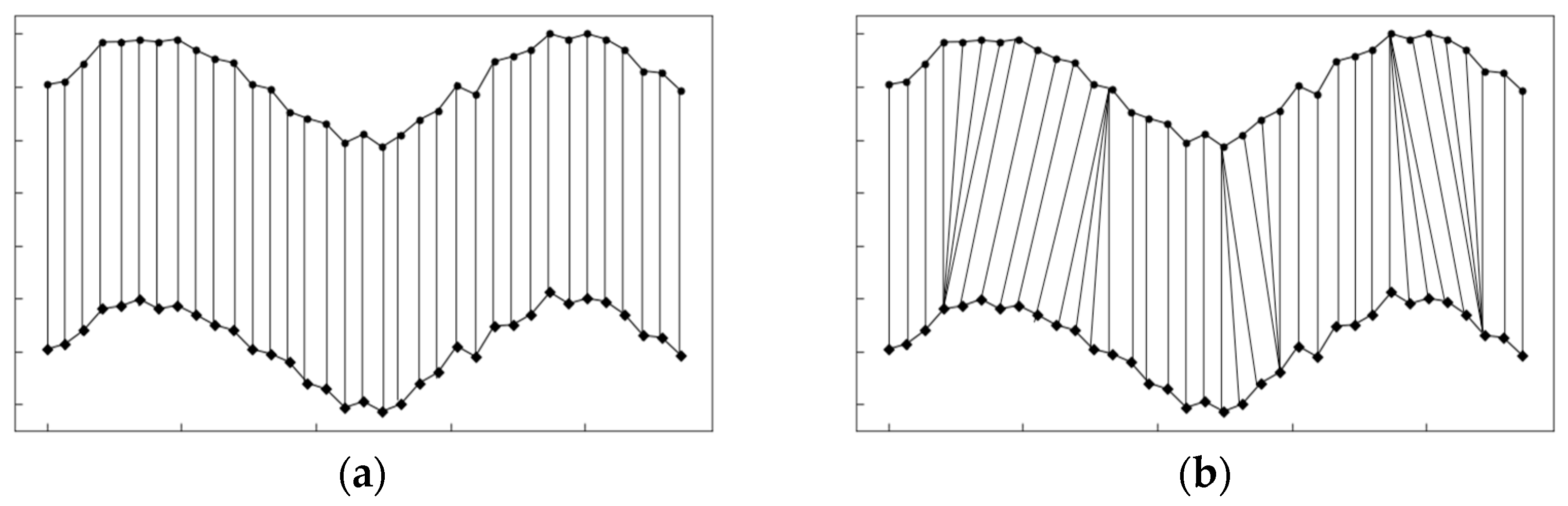It overcomes the limitations of the Euclidean distance, which arise from comparing time series of unequal lengths or with misaligned time steps, and can find the optimal matching path for time series of arbitrary lengths, thereby allowing for asynchronous matching and demonstrating strong robustness [16]. The DTW algorithm has widespread application in speech recognition, motion analysis, bioinformatics, and image recognition. Unlike the Euclidean distance, which allows for “one-to-one” alignment between two time series points, the DTW algorithm enables the accurate matching of peaks and valleys through “one-to-many” alignment (Figure 1).

Figure 1. Two different alignments: (a) one-to-one alignment (Euclidean distance) and (b) one-to-many alignment (DTW algorithm).

The DTW algorithm employs the concept of dynamic programming, ultimately aiming to identify the path to which each data point in the two time series corresponds with the minimum accumulated distance. The similarity is then defined as the average sum of the distances between corresponding grid points along the best matching path. The two time series segments are denoted as $a=\left\{a_1,a_2,\dots a_n\right\}$, $b=\left\{b_1,b_2,\dots b_m\right\}$. To align the two time series, a matrix $\mathit{M}$ of size $m\times n$ is constructed, and the distance between the corresponding points $a_i$ and $b_j$ of the two time series is denoted by the element at the (i, j) position of the matrix $\mathit{M}$, defined as

$$Dist(i,j)=\left|a_i-b_j\right|$$

(2)

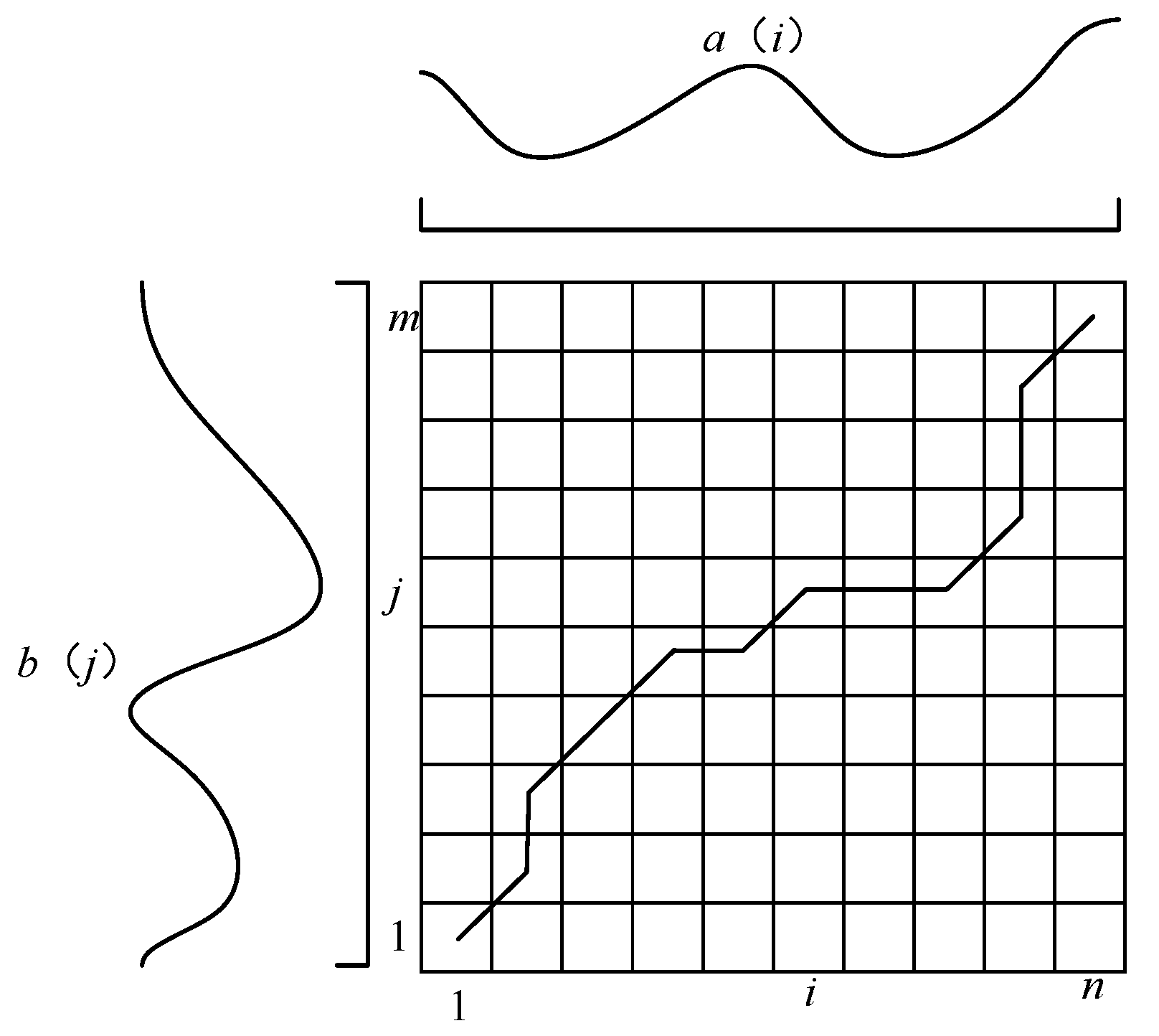
This method can be visualized as finding a path through grid points on a grid diagram (Figure 2), with the aligned points representing those visited on this path. We define this path as a warping path denoted by $W$, and the regularized path $W$ can be considered as a collection of index sequences [16]:

$$W=w_1,w_2,\dots ,w_k,\dots ,w_K$$

(3)

where $\max (m,n)\le K\le m+n+1$. This path must adhere to the following constraints [16]: (1) boundary constraint: $w_1=(1,1)$ and $w_K=(m,n)$; (2) continuity constraint: if $w_{k-1}=(a^{\prime },b^{\prime })$, then $w_k=(a,b)$ should satisfy $a-a^{\prime }\le 1$ and $b-b^{\prime }\le 1$; and (3) monotonicity constraint: if $w_{k-1}=(a^{\prime },b^{\prime })$, then $w_k=(a,b)$ should fulfill $a-a^{\prime }\ge 0$ and $b-b^{\prime }\ge 0$.

Figure 2. DTW path.

Multiple paths satisfy the aforementioned conditions. A solution is sought to determine the optimal matching path using dynamic programming and recursive methods [16].

$$D(i,j)=Dist(i,j)+\min [D(i-1,j),D(i,j-1),D(i-1,j-1)]$$

(4)

The cumulative distance $D(i,j)$ is the sum of the distance $Dist(i,j)$ from the current grid point and the cumulative distance from the nearest adjacent element to that position. Starting from the initial point of $(1,1)$ and in accordance with the three aforementioned constraints, nodes that satisfy the conditions are iteratively searched until the end point $(n,m)$ is reached, resulting in the best matching path within the matrix $\mathit{M}$. The average sum of the distance values along this final optimal matching path effectively expresses the similarity between the time series $a$ and $b$. A smaller average distance value signifies higher similarity and closer resemblance between the two time series, whereas a larger value indicates lower similarity.

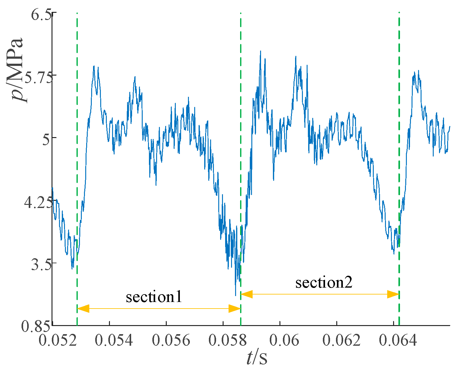
The raw signal captured by the pressure sensor on the axial piston pump is shown in Figure 3. It is evident that the waveform exhibits approximate periodicity, based on which waveform segmentation is performed. However, employing a conventional fixed-length segmentation method leads to error accumulation. To address this issue, we employ the DTW approach for waveform segmentation.

Figure 3. Time domain waveform plot of the original pressure signal.

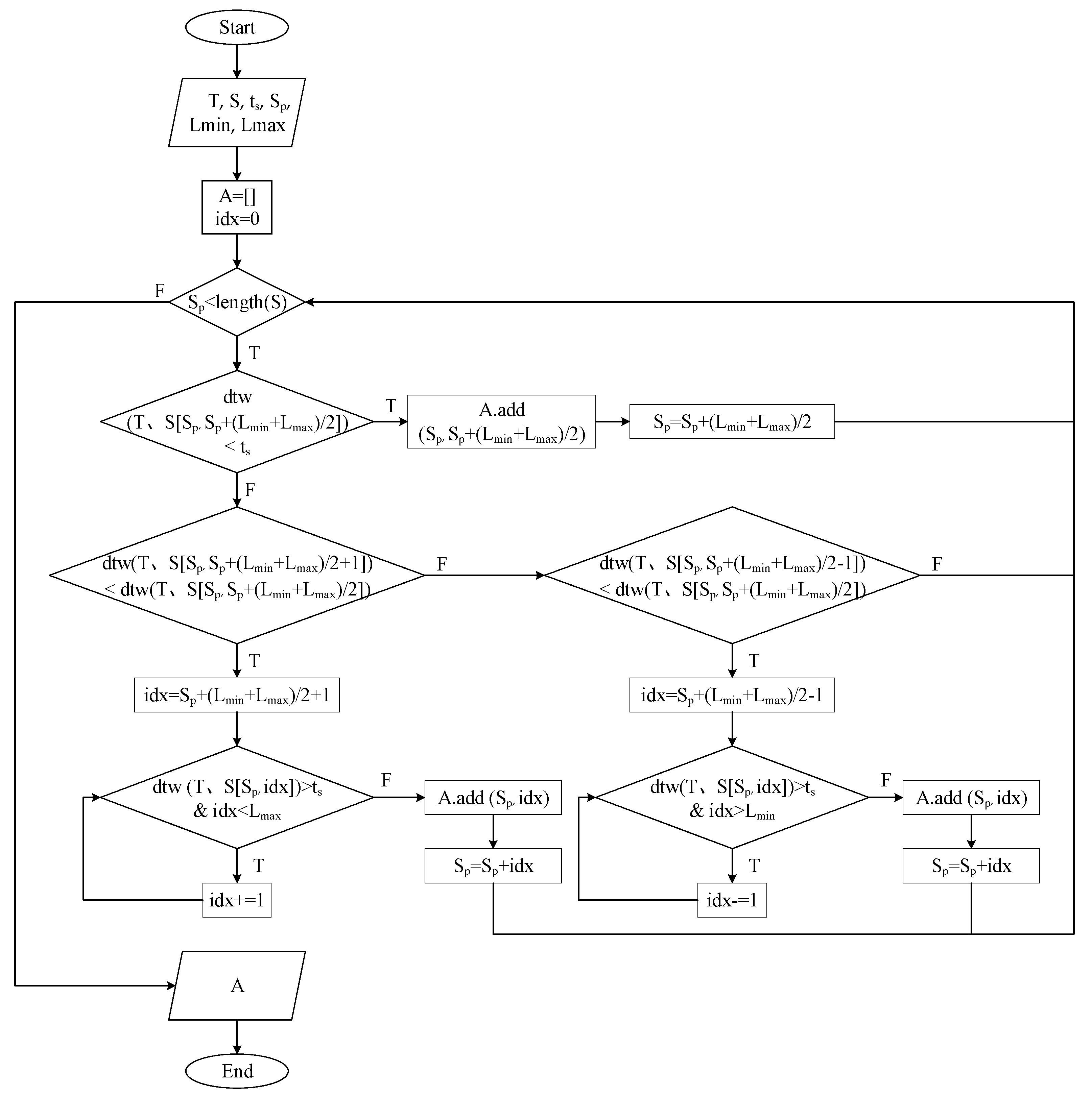
A complete pulsation cycle data segment was selected from the original pressure pulsation signal as a matching template for $T$. Subsequently, this template was used to segment the overall signal data and create a dataset. A flowchart of the algorithm is presented in Figure 4. The objective is to identify the segment within the original signal, denoted as $S$, that exhibits the highest similarity to the template $T$. To achieve this, the DTW algorithm was employed to calculate the similarity between the template and the signal, starting from a designated position, $S_p$. Throughout this process, the algorithm adhered to specific criteria, including a predefined similarity threshold $t_s$, minimum allowable output length $L_{\min }$, and maximum allowable output length $L_{\max }$. The algorithm iteratively adjusts the starting position $S_p$ based on the computed similarity. Ultimately, the output consists of a set of start and end points that define the waveform segment [14].

Figure 4. DTW algorithm divides the data flow diagram.

The DTW algorithm leverages dynamic programming and adopts a flexible path-alignment strategy to handle matching problems between time series of varying lengths. This ensures that the segmented waveforms exhibit high similarity while demonstrating robustness against noise.

3. Random Convolution Kernel

As representative algorithms in deep learning, CNNs have a wide range of applications and can be used to process data in different dimensions, including one-dimensional time series, two-dimensional images, and three-dimensional videos. One-dimensional CNNs have proven to be highly effective in processing time series data acquired from sensors. A CNN typically uses two primary components: feature extraction and pattern classification. In the feature extraction stage, convolutional and pooling layers are commonly used, often accompanied by an activation layer to enhance the extraction of key features. Subsequently, a fully connected layer is employed to perform the pattern classification task. This architectural approach enables CNNs to excel in many data-processing tasks, making them versatile tools for deep learning.

The convolutional kernel serves as the central component of the convolution layer, performing a sliding convolution operation on the input data with a step size of 1, as shown in Figure 5. This allows for weight sharing, feature extraction, and improved computational speeds. The formula for one-dimensional convolution is as follows [13]:

$$f=\mathit{w}\mathit{x}+b$$

(5)

where $\mathit{w}$ is the weight matrix of the convolution kernel, $\mathit{x}$ represents the input data, and $b$ represents the bias. CNNs employ convolutional kernels to efficiently capture diverse features and patterns within time series data through convolutional operations. The use of a large number of random convolutional kernels enhances the ability of the network to identify discriminative patterns within a time series. The essential parameters of a convolutional kernel include the length, weight, bias, kernel dilation, and padding. A substantial number of random convolution kernels were utilized to achieve an effective transformation of the time series, each configured with specific parameter values.

Figure 5. Schematic diagram of a one-dimensional convolution operation.

The lengths of the convolutional kernels were randomly selected with equal probability from among $\left\{7,9,11\right\}$, and the lengths used were typically much shorter than those of the input time series.

The weights $w_i$ of the convolutional kernels were randomly drawn from a standard normal distribution. These weights are generally modest in magnitude but can potentially assume larger values.

$$\forall w_i ϵ \mathit{w}, w_i\sim N(0, 1)$$

(6)

where $\mathit{w}$ is the weight matrix of the convolution kernel.

The bias term $b$ is determined through random sampling from a uniform distribution, $b \sim U\left(-1, 1\right)$. Notably, distinct bias values were assigned, even when dealing with convolutional kernels that were otherwise similar. This biased divergence contributed to the extraction of diverse features from the input data.

The kernel dilation parameter is pivotal to effectively enable a convolution kernel to capture patterns or features across diverse scales. The dilation rate $d$ for kernel dilation was determined by random sampling, which typically follows the following distribution:

$$d=\lfloor 2^x\rfloor , x\sim U\left(0, A\right),A={\log }_2\frac{l_{input}-1}{l_{kernel}-1}$$

(7)

where $l_{input}$ is the length of the input data and $l_{kernel}$ is the length of the convolution kernel. This random sampling of the dilation rate ensures that the convolution kernel can accommodate patterns or features with varying frequencies and scales. Furthermore, during the generation of each convolutional kernel, a random decision (with equal probability) is made to determine whether a padding operation should be performed. If padding is selected, a certain amount of zero padding is added at the beginning and end of the input time series when the convolution kernel is applied. This ensures that the “center” element of the convolution kernel aligns with every point in the time series. Padding aims to adjust the alignment between the input data and the convolution kernel, thereby enhancing the capture of patterns and features from the time series. The stride of the convolution kernel was maintained at one.

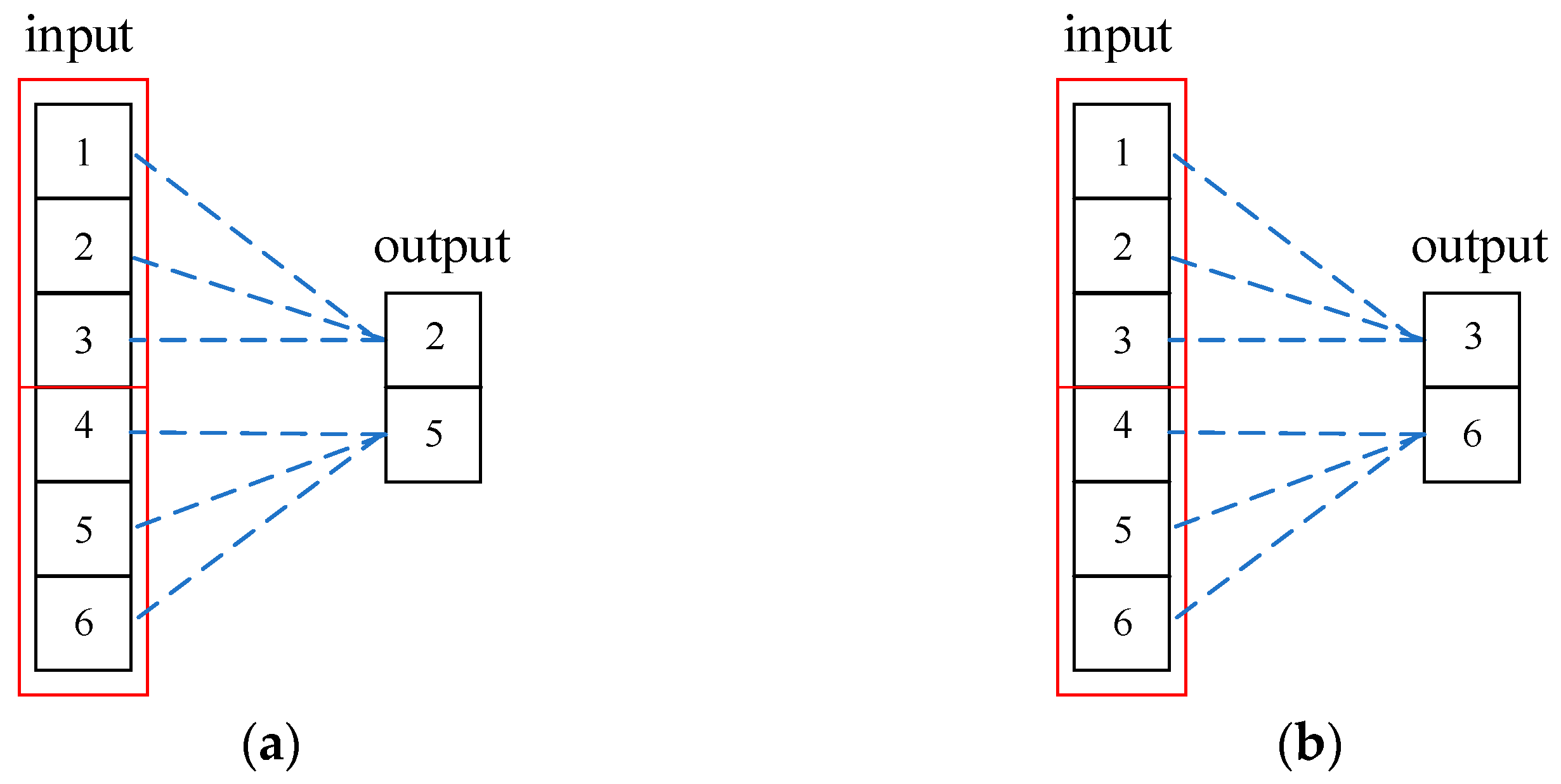
The pooling layer, which can be divided into two types of operations, average pooling and maximum pooling, is shown in Figure 6.

Figure 6. Schematic diagram of pooling: (a) average pooling; (b) maximum pooling.

Feature extraction was accomplished using a set of 1000 one-dimensional random convolution kernels. Two aggregate features are computed from each feature map to yield two real values for each convolution kernel. These two features are the maximum value obtained through maximum pooling and the proportion of positive values in $p$. The proportion of positive values $p$ is defined as the ratio of positive elements in the output obtained after the convolution operation and is calculated using the following formula:

$$p\left(\mathit{z}\right)=\frac{1}{m}{\displaystyle {\sum }_{j=0}^{m-1}(z_j>0)}$$

(8)

where $\mathit{z}$ is the output of the convolution operation, and $z_j$ is the $j$th element in $\mathit{z}$. Specifically, $(z_j>0)$ is an indicator function that takes the value of 1 when $z_j$ is greater than 0 and 0 otherwise. The maximum value reflects the global features following transformation by random convolutional kernels and is sensitive to abnormal features. However, the proportion of positive values in $p$ signifies the degree of correspondence between the input data and locally detected abnormal features captured by the random convolutional kernel. After maximum pooling and the feature extraction layer, 1000 convolutional kernels generate 2000 feature values, thereby forming a feature dataset.

4. Anomaly Detection

4.1. One-Class Support Vector Machine

With the evolution of support vector machines, two distinct algorithms have emerged: the support vector data description (SVDD) algorithm, often referred to as the hypersphere method, and the one-class support vector machine (OCSVM) algorithm, commonly known as the hyperplane method. The underlying principle of the OCSVM algorithm is as follows [17]: a hyperplane is found in a higher-dimensional space to perform the linear separation of the original data samples mapped in this space. This process involves the initial establishment of a hyperplane $\mathit{w}\cdot \mathsf{\Phi }(\mathit{x})-\rho =0$ and the subsequent maximization of the distance $\rho /\parallel \mathit{w}\parallel$ between the target data sample and the origin. This approach determines the optimal hyperplane, as shown in Figure 7.

Figure 7. Optimal hyperplane for OCSVM.

In the hyperplane method, the optimization problem is solved as follows [17]:

$$\begin{array}{c}\underset{w,\rho ,{\xi }_i}{\min }\frac{1}{2}\parallel \mathit{w}{\parallel }^2+\frac{1}{\nu l}{\displaystyle {\displaystyle \sum }_{i=1}^l}{\xi }_i-\rho \\ s.t.\mathsf{\Phi }({\mathit{x}}_i)\mathit{w}\ge \rho -{\xi }_i,{\xi }_i\ge 0,i=1,2,\dots ,l\end{array}$$

(9)

where ${\mathit{x}}_i$ is the training sample; $\mathsf{\Phi }: \mathrm{X}\to H$ signifies the mapping relationship between the original space and the high-dimensional feature space; $\mathit{w}$ and $\rho$ are the parameters of the hyperplane; $\xi$ represents a slack variable; $\nu$ is a balancing parameter used to adjust the degree of relaxation; and $l$ is the number of training samples. The dual form of the optimization problem is as follows [17]:

$$\begin{array}{c}\underset{\alpha }{\min } \frac{1}{2}{\displaystyle {\displaystyle \sum }_i^l}{\displaystyle {\displaystyle \sum }_j^l}{\alpha }_i{\alpha }_{j}K({\mathit{x}}_i,{\mathit{x}}_j)\\ s.t. 0\le {\alpha }_i\le \frac{1}{\nu l},{\displaystyle {\displaystyle \sum }_i^l}{\alpha }_i=1,i=1,\dots ,l\end{array}$$

(10)

where ${\alpha }_i$ is the Lagrange factor. The final decision function is [17]

$$f(\mathit{x})=\mathrm{sign}({\displaystyle \sum }_i^l{\alpha }_i^{\ast }K({\mathit{x}}_i,\mathit{x})-\rho )$$

(11)

where ${\alpha }_i^{\ast }$ corresponds to the vector, and ${\mathit{x}}_i$ is the support vector. A sample point was considered normal when it was $f(\mathit{x})>0$; otherwise, it was considered abnormal.

4.2. Isolation Forest

An isolation forest is an integrated learning approach based on a decision tree model. Its underlying principles possess similarities with those of the random forest algorithm; however, it distinguishes itself by employing a fully randomized process to generate isolated binary trees. This algorithm is highly regarded for its robustness with regard to noise, its low computational complexity, its ability to handle extensive datasets, and its proficiency with high-dimensional feature spaces. Consequently, it is exceptionally well suited for anomaly detection, particularly when applied to features extracted from the random convolution kernels of a CNN. By randomly partitioning the dataset, this algorithm can separate anomalous points using a few cuts, whereas normal points require more cuts to be distinguished. In an isolated tree, normal samples typically reside deeper within the tree structure, while abnormal samples tend to reside closer to the tree root. The tree depth corresponds to the number of partitions performed. The core of the algorithm lies in the construction of an isolation tree, which is structured into leaf, inner, and root nodes, as depicted in Figure 8.

Figure 8. Schematic diagram of an isolation tree structure.

The isolation forest algorithm initially generates $n$ isolation trees, which are then assembled into an isolation forest model. Subsequently, an anomaly score is computed for each data sample. The algorithm accomplishes the anomaly detection task primarily based on the path length of the data points. This method is well known for its simplicity and efficiency. Figure 8 illustrates that “triangle-shaped” samples have the shortest path lengths, making them more likely to be classified as anomalies. Anomaly scores are calculated as follows [14]:

$$c\left(n\right)=2H(n-1)-\frac{2(n-1)}{n}$$

(12)

where $c(n)$ is the average path length of the $n$ isolation trees, and $H(i)$ is the harmonic number, approximated as $\ln \left(i\right)+0.5772156649$. The anomaly score function is expressed as follows:

$$s(x_i,n)=2^{-\frac{E[h(x_i)]}{c(n)}}$$

(13)

where $s(x_i,n)$ represents the anomaly score of sample $x_i$, $h(x_i)$ denotes the path length of sample $x_i$, and $E[h(x_i)]$ is the expectation of the path length of $x_i$ for all isolation trees.

Furthermore, the relationship between $E[h(x_i)]$ and $s(x_i,n)$ was obtained, as shown in Figure 9. There are three cases:

$$\begin{array}{l}E[h(x_i)]\to 0,s(x_i,n)\to 1;\\ E[h(x_i)]\to n-1,s(x_i,n)\to 0;\\ E[h(x_i)]\to c(n),s(x_i,n)\to 0.5\end{array}$$

(14)

Figure 9. Relationship between E[h(x_i)] and s(x_i, n).

The sample was considered abnormal if the anomaly score was close to 1 and it was considered normal if the anomaly score was <0.5.

5. Axial Piston Pump Simulation Test

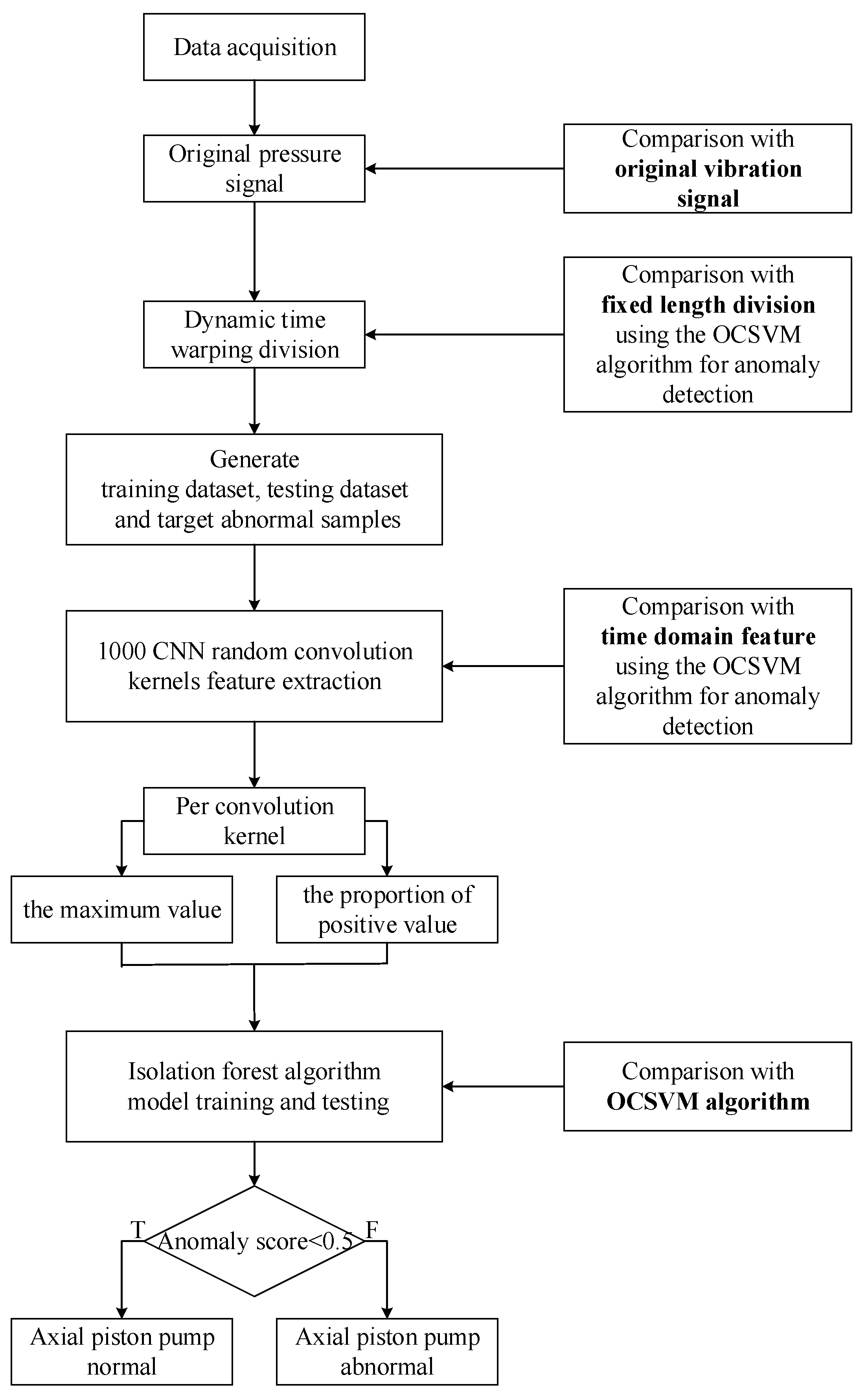
The process of axial piston pump anomaly detection is illustrated in Figure 10. First, the axial piston pump outlet pressure signal and end cap vibration signal were collected. Second, the collected original pressure signal was divided using the DTW algorithm to generate the dataset. Then, 1000 CNN random convolution kernels were used to carry out feature extraction from the divided data, and each convolution kernel was extracted to the maximum value and the proportion of the positive values of the two feature values. A total of 2000 features were extracted from 1000 random convolution kernels, and anomaly detection using the isolation forest algorithm was carried out.

Figure 10. Flowchart of anomaly detection method.

Unlike the traditional CNN approach, this method avoids adding extra convolutional layers or pursuing depth expansion. Instead, its scope was widened by increasing the number of convolutional kernels through a random selection of their parameters. This expansion can effectively capture discriminative patterns within time series data. A comparative test for a comprehensive evaluation of the performance of the model was conducted using the originally captured vibration signals.

5.1. Experimental Platform

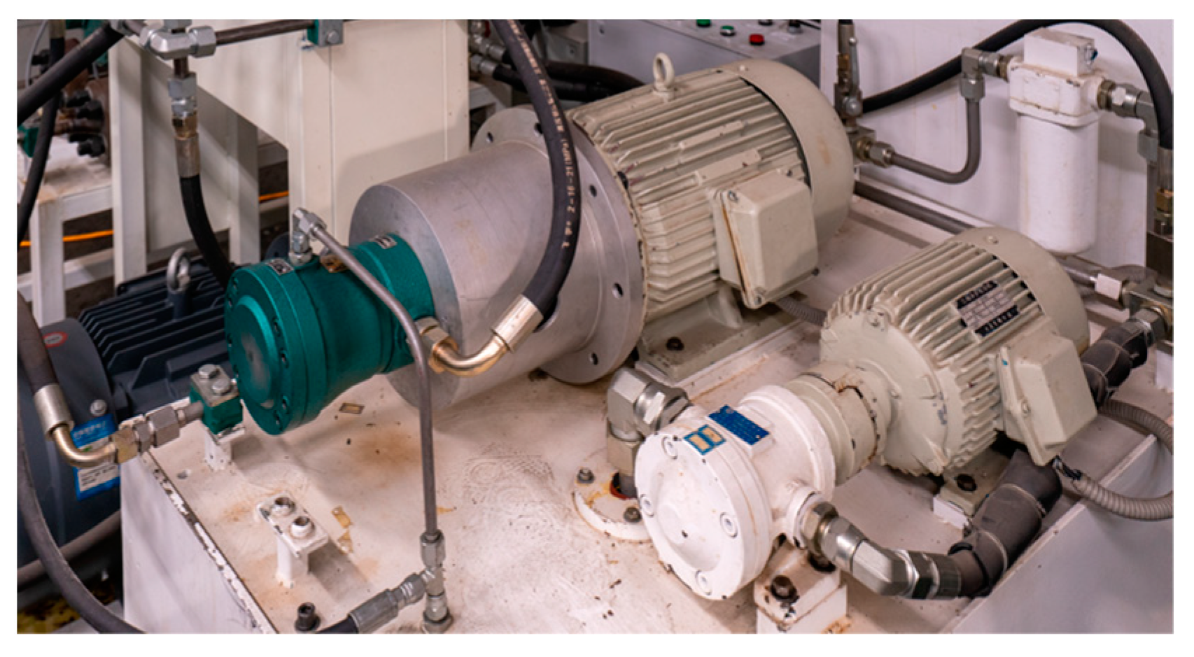
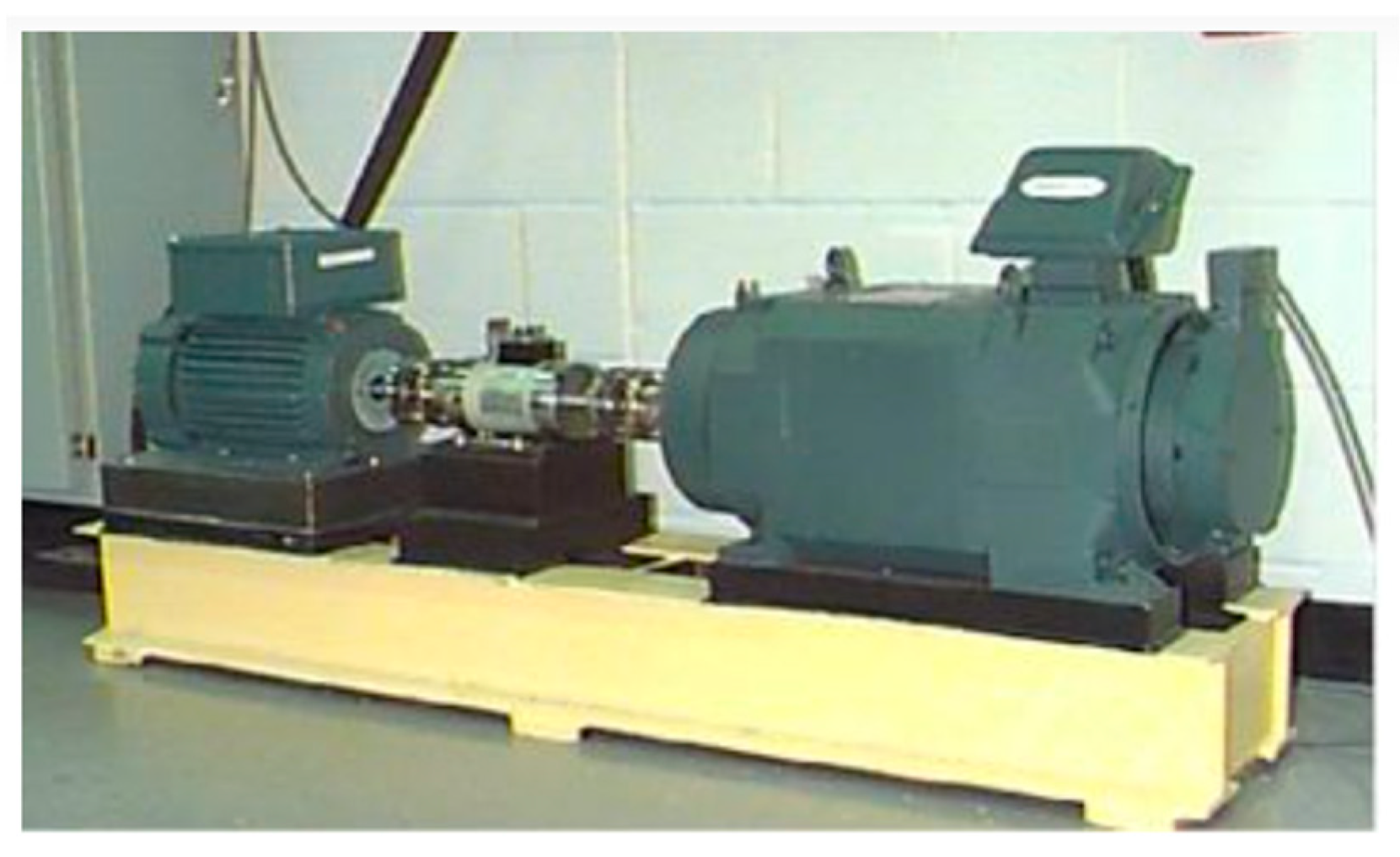
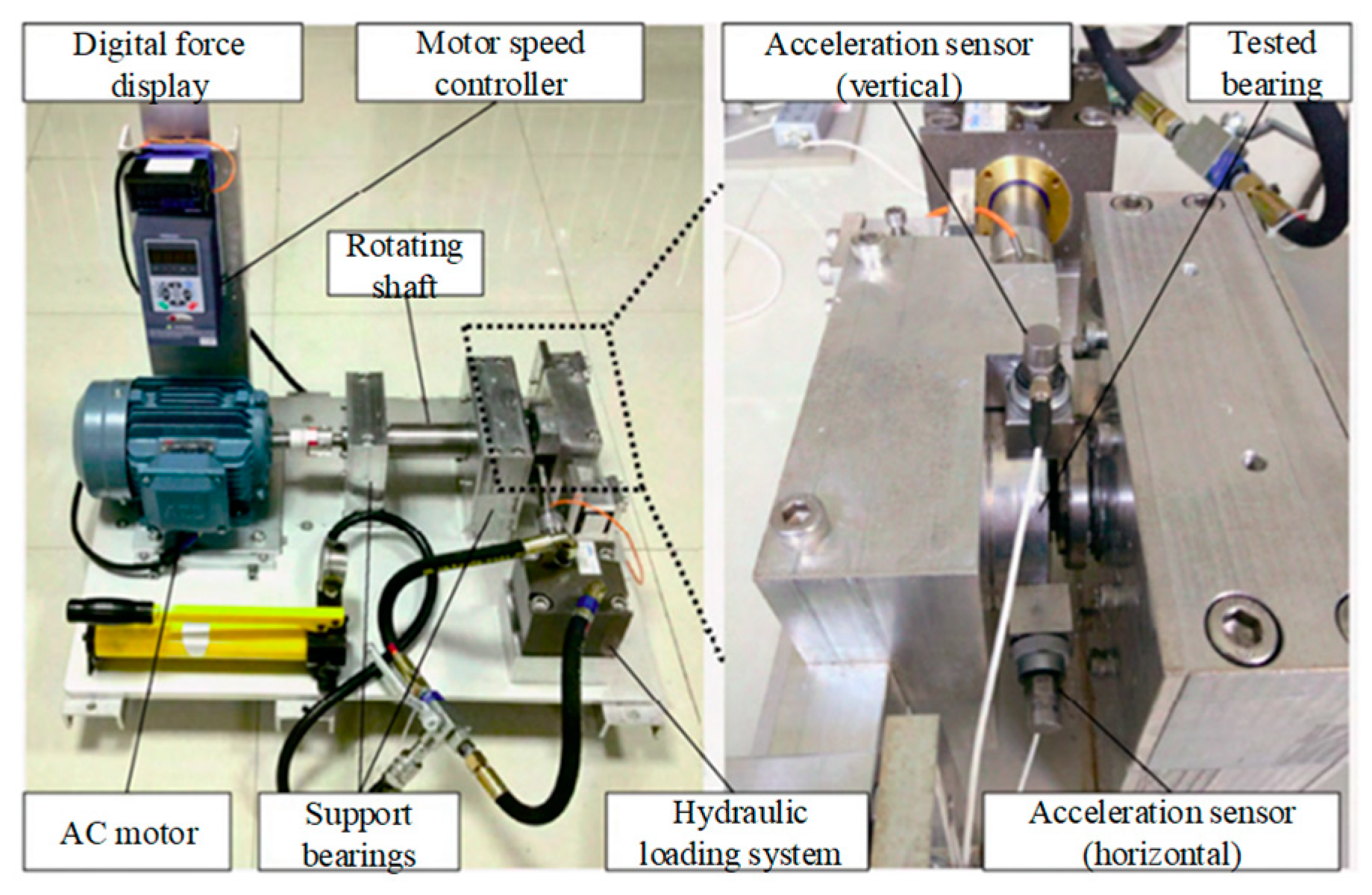
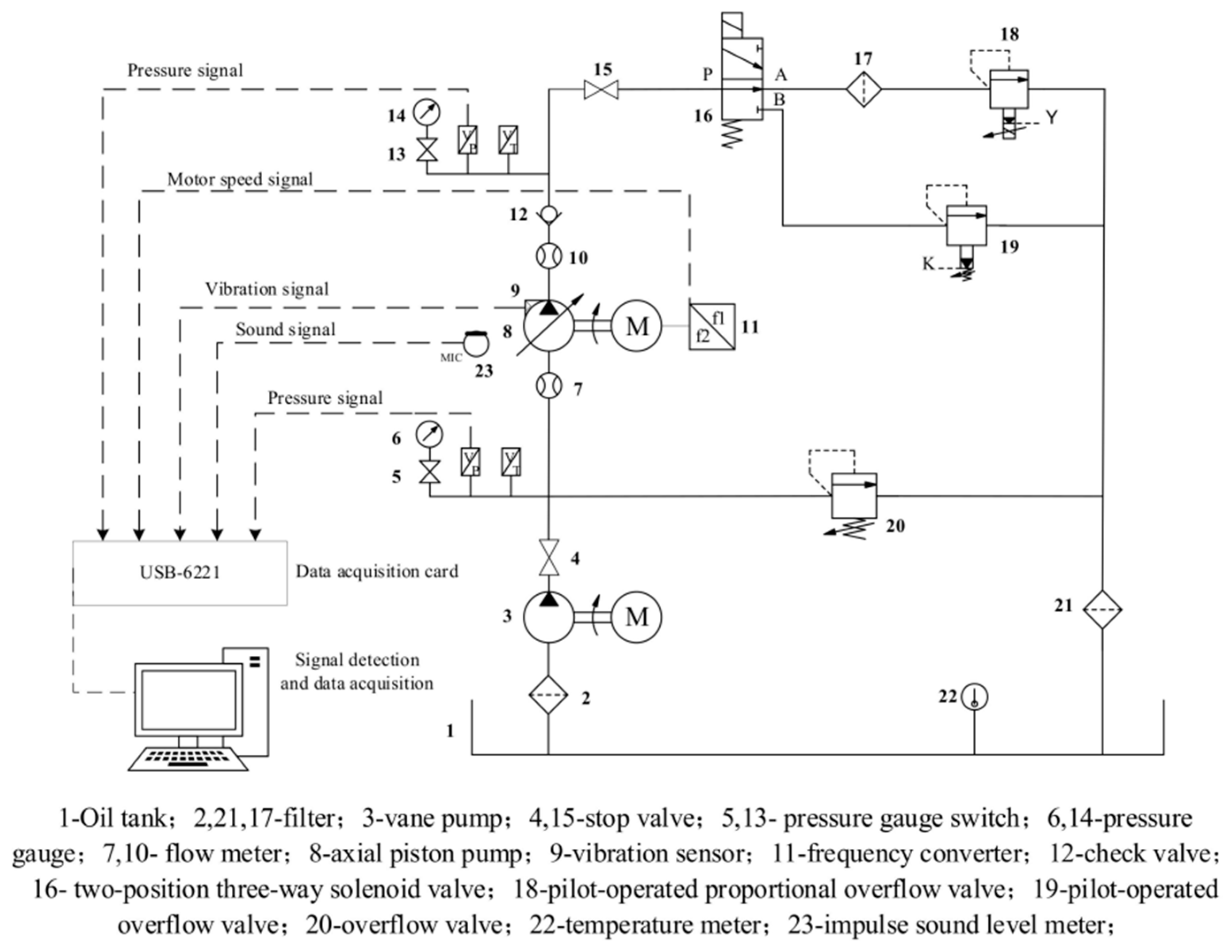
In this study, simulation tests were conducted to detect anomalies in axial piston pumps using a specialized testbed designed for axial piston pump failure simulations, as illustrated in Figure 11. The test bed was equipped with a pressure sensor positioned at the outlet of the axial piston pump to record pressure signals. Additionally, three vibration acceleration sensors were strategically placed in mutually perpendicular directions (x, y, and z) on the end cover and casing of the axial piston pump to capture vibration signals. Simultaneously, the LabView 2021 software facilitated the monitoring of the operational state of the axial piston pump, enabling the collection of experimental data. A schematic of the experimental setup is shown in Figure 12.

Figure 11. Axial piston pump failure simulation test bench.

Figure 12. Schematic diagram of the experimental setup for simulation of faults in an axial piston pump.

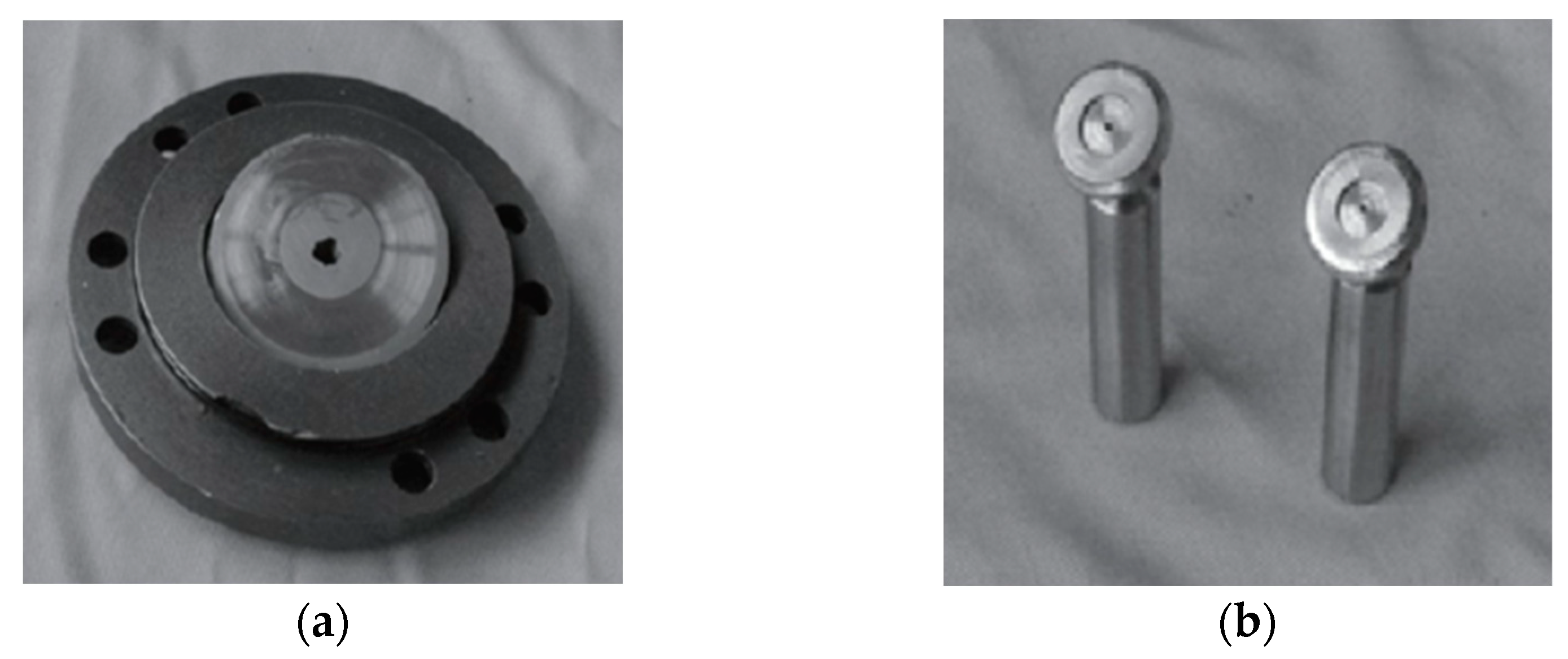
The axial piston pump used in the experiment was an MCY14-1B model with displacement of 10 mL/r. The drive motor was a Y132M4 model with a rated rotational speed of 1480 rpm. Data acquisition was facilitated using an NI-USB-6221 data acquisition card with a maximum sampling rate of 250 kS/s. The pressure transducer used was the PT124B-210-40MPa-GB model, covering a pressure range of 0–40 MPa. The vibration acceleration transducer was a YD72D model with a frequency range of 1 Hz–18 kHz. In the test, artificial faults were introduced by substituting standard components with faulty components through fault injection. Three types of abnormal states were simulated: swashplate wear (artificially inducing wear on the swashplate), sliding shoe wear (removing rounded edges), and single-plunger loose shoe wear (faulty component). The faulty components are depicted in Figure 13. The data collected for the experiment, including those of the normal and three different abnormal states, were obtained under system pressure of 5 MPa. The sampling frequency was set to 50 kHz, with each sampling lasting 1 s.

Figure 13. Pictures of the faulty elements: (a) swashplate wear and (b) sliding shoe wear.

5.2. Comparative Analysis of Experimental Data

5.2.1. Data Acquisition

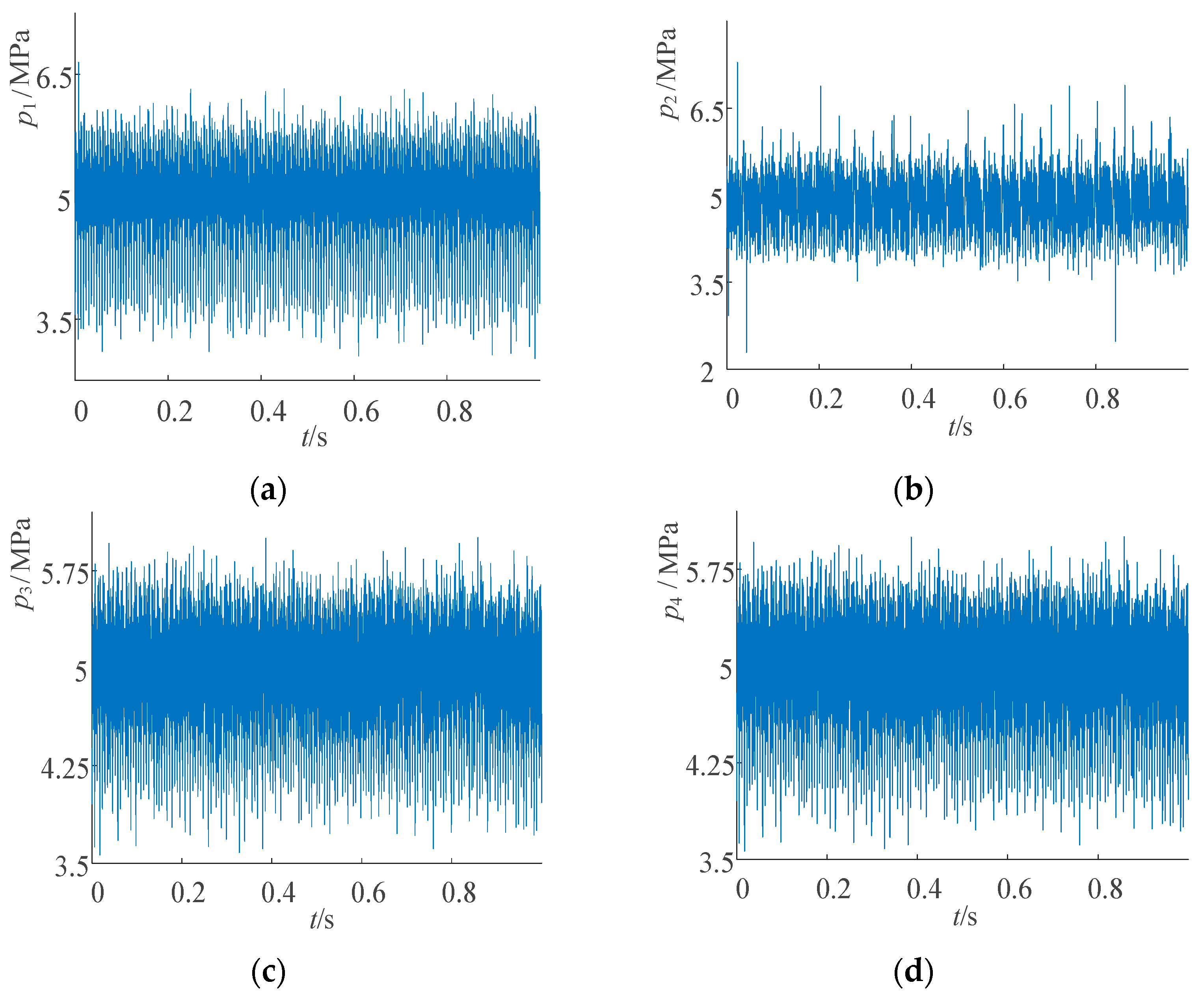
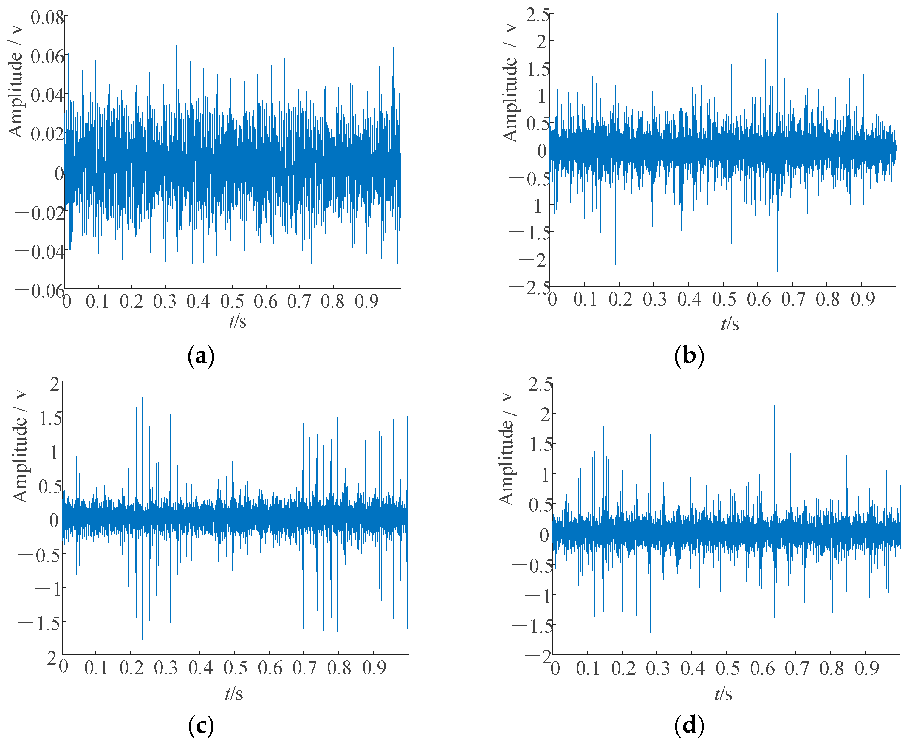
The pressure signals at the pump outlet were collected under four conditions: normal, swashplate wear, sliding shoe wear, and single-plunger loose shoe. The testing conditions were consistent, resulting in time domain waveforms of the original pressure signals for each of the four operating conditions, as shown in Figure 14. The sequence length for all four conditions was 50,000 data points.

Figure 14. Time domain waveform plot of the raw pressure signal: (a) normal; (b) swashplate wear; (c) sliding shoe wear; (d) single-plunger loose shoe.

5.2.2. Performance Comparison of Different Data Partitioning Methods

As shown in Figure 14, it is challenging to determine the health status of an axial piston pump through a direct visual inspection of the time domain waveform of the pressure signal. To address this challenge, the DTW algorithm was deployed to segment the data and construct a dataset. To validate the effectiveness of the DTW algorithm for data partitioning, an additional dataset was generated using the same processing method as used in the fixed-length partitioning approach. Subsequently, the OCSVM algorithm was applied to perform anomaly detection on the datasets obtained using the two data-partitioning methods. The detection results are compared to ascertain the advantages of the DTW algorithm.

Division of DTW Method

A complete pulsation cycle segment was selected as the matching template, and the DTW algorithm was applied in the partitioning of the dataset according to the process outlined in Figure 4. The number of data points in each partitioned complete pulsation cycle signal varied. For ease of processing, the median length of all data segments (289) was selected as the standard sequence. Segments longer than 289 were truncated from the beginning, whereas segments shorter than 289 were padded from the end. Data partitioning was conducted on data collected under normal operating conditions, resulting in 164 samples. The training and testing datasets were split in a 3:1 ratio, yielding 123 and 41 samples for the training and testing sets, respectively. After completing data partitioning for the three abnormal operating states, 41 random samples were selected as the target abnormal samples. The partitioning results are listed in Table 1.

Table 1. Axial piston pump pressure signal data set DTW partition.

Category	Sample Length	Number of Samples	Training Dataset	Testing Dataset	Target Abnormal Samples
normal	289	164	123	41	-
swashplate wear	289	165	0	-	41
sliding shoe wear	289	164	0	-	41
single-plunger loose shoe	289	164	0	-	41

Fixed Length Division

Following the data-partitioning approach outlined in Table 1, the axial piston pump pressure signal dataset was divided into fixed-length segments of 289 for all four operating conditions. The aforementioned processing method was used to generate the dataset.

OCSVM Anomaly Detection

Anomaly detection was performed on the datasets generated by the two aforementioned segmentation methods using the OCSVM algorithm. The results were evaluated using standard machine learning metrics, including the precision, recall, and F1 scores, as presented in Table 2.

Table 2. Performance comparison of different data partitioning methods.

Method	Fixed-Length Division			DTW Division
	P	R	F1	P	R	F1
normal	100.00	24.39	39.22	100.00	58.54	73.85
swashplate wear	56.94	100.00	72.57	70.69	100.00	82.83
sliding shoe wear	56.94	100.00	72.57	70.69	100.00	82.83
single-plunger loose shoe	56.94	100.00	72.57	70.69	100.00	82.83
average	67.71	81.10	64.98	78.02	89.64	80.59

The results indicate that when fixed-length data division was employed, the average precision for the four working conditions was 67.71%, with an average recall rate of 81.10% and an average F1 score of 64.98%. In contrast, using DTW for data division yielded average precision of 78.02%, average recall of 89.64%, and an average F1 score of 80.59% across the four working conditions. A close examination revealed that the F1 score exhibited an average increase of 15.61% when DTW was employed in the data division. This method demonstrates robust adaptability by discerning the optimal warping path to closely match data segments with high adaptability and robustness, thereby allowing for the preservation of more information from the original signal and improving the overall algorithm’s precision.

5.2.3. Performance Comparison of Different Feature Extraction Methods

The dataset postsegmented using DTW was directly utilized for anomaly detection using the OCSVM algorithm. Each sample within this dataset comprises continuous time series data encompassing many sampling points. Considering the inherent continuity and high dimensionality of the data, anomaly detection often entails high computational complexity. Consequently, feature extraction was conducted on the segmented data to extract the relevant features. This feature extraction process serves several critical objectives, including bolstering the model’s generalization capabilities, optimizing the computational efficiency, and, most importantly, enhancing the precision of the detection outcomes.

Conventional time domain feature extraction was performed on the partitioned dataset, resulting in a collection of extracted time domain features. This feature set comprised eight quantitative characteristics: maximum, minimum, peak, mean, variance, standard deviation, mean square, and root mean square. In addition, it encompassed six dimensionless features, namely kurtosis, skewness, the waveform factor, the peak factor, the impulse factor, and the margin factor—totaling 14 feature parameters. Subsequently, while ensuring that essential information was retained, principal component analysis (PCA) was employed to reduce the dimensionality of the dataset. After the dimensionality reduction, the number of principal components was set to four.

Deep learning offers substantial advantages in feature extraction. When a CNN with random convolutional kernels is used for feature extraction, it automatically learns the features present in the data specific to the task. The combination of numerous random convolutional kernels effectively captures discriminative patterns in time series data. For the dataset obtained by applying the DTW algorithm for partitioning and matching, feature extraction was performed using a CNN with random convolutional kernels. To generate the 2000 feature dimensions that comprised the feature dataset, 1000 one-dimensional random convolutional kernels were selected. Subsequently, the two feature datasets obtained from the distinct feature extraction methods were subjected to anomaly detection using the OCSVM algorithm. The results presented in Table 3 validate the advantages of the CNN with random convolutional kernels for feature extraction.

Table 3. Performance comparison of different feature selection methods.

Feature	Traditional Time Domain Feature + PCA			Random Convolution Kernels Feature Extraction
	P	R	F1	P	R	F1
normal	100.00	65.85	79.41	100.00	82.93	90.67
swashplate wear	74.55	100.00	85.42	85.42	100.00	92.13
sliding shoe wear	74.55	100.00	85.42	85.42	100.00	92.13
single-plunger loose shoe	74.55	100.00	85.42	85.42	100.00	92.13
average	80.91	91.46	83.92	89.07	95.73	91.77

The results demonstrate that feature extraction from the divided dataset, when compared with the time domain features, led to an average increase of 8.16% in precision, a 4.27% boost in recall, and a remarkable 7.85% improvement in the average F1 score. This indicates that feature extraction using the CNN with random convolution kernels significantly enhanced the information content derived from the original data. The extraction method for time domain features often adopts a global perspective, whereas CNNs with random convolution kernels prioritize local feature characteristics during the convolution process. This enhances the algorithmic efficiency and fortifies the robustness and generalization capabilities of the model.

5.2.4. Performance Comparison of Different Anomaly Detection Methods

Both the OCSVM and isolation forest algorithms are frequently employed for anomaly detection. The OCSVM algorithm maps data onto a high-dimensional space and aims to find the optimal hyperplane that maximizes the distance between the training samples and the origin as much as possible. By contrast, the isolation forest algorithm uses a randomized data segmentation approach, which is known for its high computational efficiency. When anomaly detection is performed, the advantages of different algorithms are comprehensively considered, and an appropriate algorithm is selected to obtain more accurate and reliable anomaly detection results. The two anomaly detection methods were compared, and the results are listed in Table 4.

Table 4. Performance comparison of different anomaly detection methods.

Method	OCSVM			Isolation Forest
	P	R	F1	P	R	F1
normal	100.00	65.85	79.41	100.00	73.17	84.51
swashplate wear	74.55	100.00	85.42	78.85	100.00	88.17
sliding shoe wear	74.55	100.00	85.42	78.85	100.00	88.17
single-plunger loose shoe	74.55	100.00	85.42	78.85	100.00	88.17
average	80.91	91.46	83.92	84.14	93.29	86.51

The findings indicate that anomaly detection using the isolation forest algorithm yields an average increase of 3.23% in precision, 1.83% in recall, and 2.59% in the F1 score compared with the OCSVM algorithm. The isolation forest algorithm, built upon decision tree principles, exhibits notable strengths when dealing with large-scale datasets and shows enhanced robustness against noise and diverse anomaly types. Therefore, the use of the isolation forest algorithm for anomaly detection offers superior detection performance compared with the OCSVM algorithm.

5.3. Performance of the Proposed DTW-RCK-IF Composite Method in This Article

5.3.1. Overall Performance

Following the aforementioned comparative validations, it was found that compared to the fixed-length partitioning method, the DTW algorithm for data partitioning yielded more similar data segments. In contrast to traditional time domain feature extraction and dimensionality reduction methods, the random convolutional kernel feature extraction method of the CNN was proven to be more effective in capturing local features in time series data, thereby enhancing the model generalization and robustness. Furthermore, compared with the OCSVM algorithm, the isolation forest anomaly detection method demonstrated excellent performance for large-scale datasets and high-dimensional feature spaces. The operational data of axial piston pumps are typically manifested as time series data. Considering the dynamism and variability within the data, the DTW algorithm was introduced to delineate matching data patterns. The CNN, which automatically extracts features and captures local patterns from time series data, proved effective in discerning key features for enhanced anomaly detection. The incorporation of random convolutional kernels introduced a degree of randomness that fostered model diversity and robustness. This became particularly significant in the context of potentially complex patterns and noise within the axial piston pump data, thereby improving the adaptability of the model. The isolation forest algorithm is an effective anomaly detection method that can swiftly and accurately identify anomalous samples. Given the critical nature of promptly detecting abnormal patterns or fault states in data collected from axial piston pumps, the isolation forest algorithm provides valuable support. In summary, the combination of DTW, a CNN with random convolutional kernels, and the isolation forest algorithm effectively leverages their respective strengths. This combination proved to be highly applicable to the anomaly detection problem of axial piston pumps. These methods handle time series data in depth, automatically extract features, enhance model robustness, and facilitate efficient anomaly detection. Consequently, the final experiment adopted the DTW-RCK-IF composite method for anomaly detection. A baseline comparison was performed with traditional anomaly detection methods, such as the LOF, OCSVM, and isolation forest algorithms, and the results are presented in Table 5.

Table 5. Results of anomaly detection using the DTW-RCK-IF method.

Method	LOF			OCSVM			Isolation Forest			DTW-RCK-IF
	P	R	F1	P	R	F1	P	R	F1	P	R	F1
normal	100.00	63.41	77.61	100.00	65.85	79.41	100.00	73.17	84.51	100.00	97.56	98.77
swashplate wear	73.21	100.00	84.54	74.55	100.00	85.42	78.85	100.00	88.17	97.62	100.00	98.80
sliding shoe wear	73.21	100.00	84.54	74.55	100.00	85.42	78.85	100.00	88.17	97.62	100.00	98.80
single-plunger loose shoe	73.21	100.00	84.54	74.55	100.00	85.42	78.85	100.00	88.17	97.62	100.00	98.80
average	79.91	90.85	82.81	80.91	91.46	83.92	84.14	93.29	86.51	98.22	99.39	98.79

The results show that the anomaly detection method combining the DTW algorithm and random convolutional kernel feature extraction, as well as the isolation forest algorithm, has an average of 98.22% precision, 99.39% recall, and 98.79% F1 score for the four working conditions compared with the isolation forest algorithm. For the same dataset, the average precision increased by 14.08%, the average recall increased by 6.1%, and the average F1 score increased by 12.28%. This further validates the superior performance of the CNN with random convolutional kernels for feature extraction. This also underscores the enhanced capability of the method in recognizing normal data and its high accuracy in identifying various abnormal states, thereby affirming its robustness. Further analysis of the DTW-RCK-IF composite method showed that the recall of this method for abnormal data could be as high as 100%, whereas that for normal data was only 97.56%. The reason for this may be that there are minor differences between the features of misjudged normal data and those of abnormal data, and there are precursors to failure in normal data, which indicates that this method is more sensitive to abnormal data and has a stronger recognition ability. Based on a comprehensive analysis of the aforementioned results, the DTW-RCK-IF composite method exhibits significant advantages over other traditional anomaly detection algorithms. This method consistently outperformed alternative approaches in terms of the precision, recall, and F1 score metrics. The DTW-RCK-IF composite method demonstrated robust identification capabilities across normal, swash plate wear, sliding shoe wear, and single-plunger loose shoe data. This further confirms the superiority of the proposed method.

5.3.2. Parameter Sensitivity

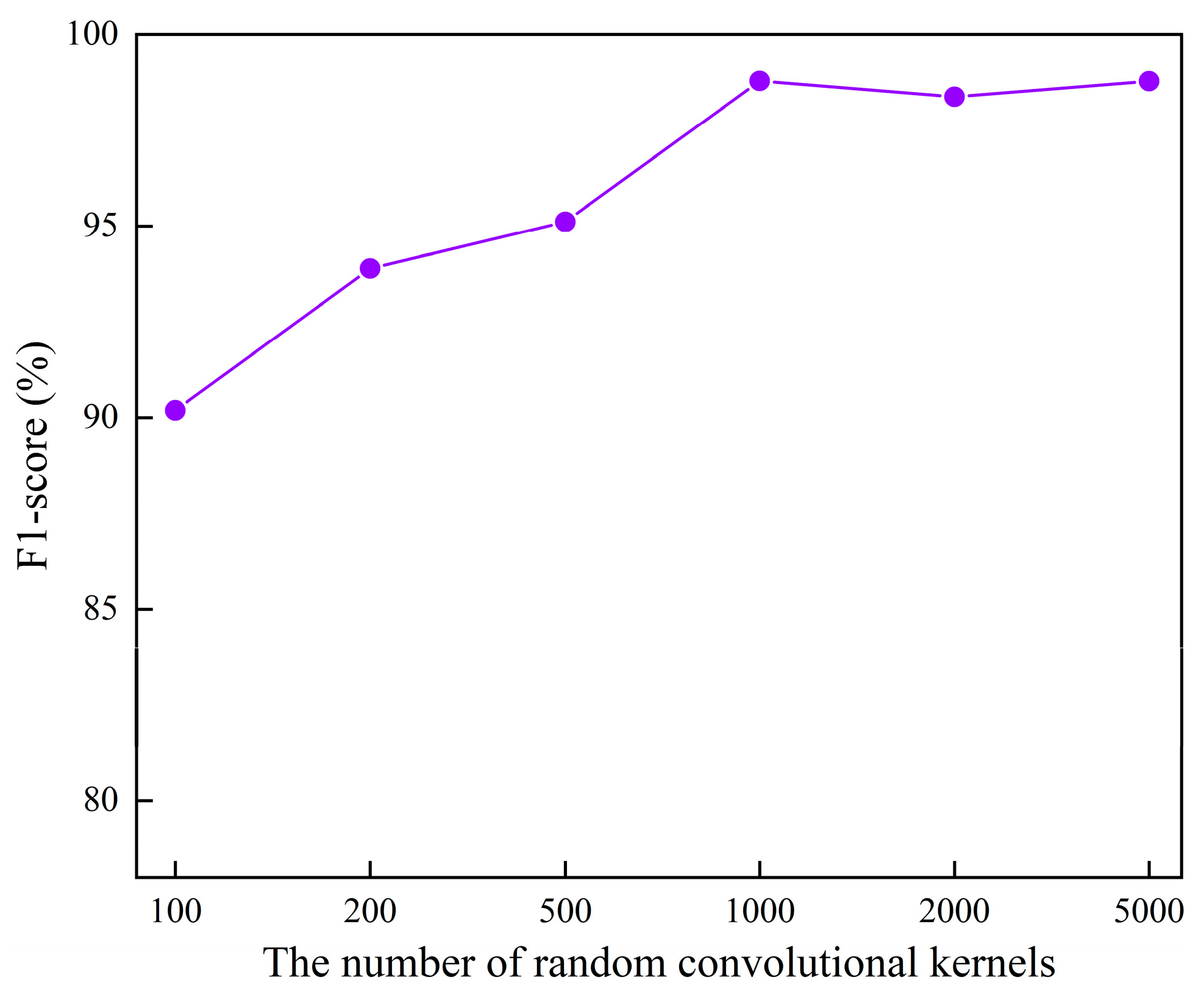
We investigated the effect of the number of random convolutional kernels (100, 200, 500, 1000, 2000, and 5000) on the overall performance of the proposed method. Figure 15 illustrates the model performance for different random convolutional kernel numbers. It can be observed that increasing the number of kernels effectively enhanced the model performance as long as the number remained below 1000. The model achieved optimal performance when the number of kernels reached 1000, demonstrating high classification accuracy. However, as the number of kernels continued to increase to beyond 1000, the variation in the model performance became relatively small. Therefore, we selected 1000 as the number of random convolutional kernels for this method. These results validate the sensitivity of the proposed method, which is essential for practical applications.

Figure 15. Effect of parameters.

5.4. Comparing the Detection Performance of Pressure and Vibration Signals

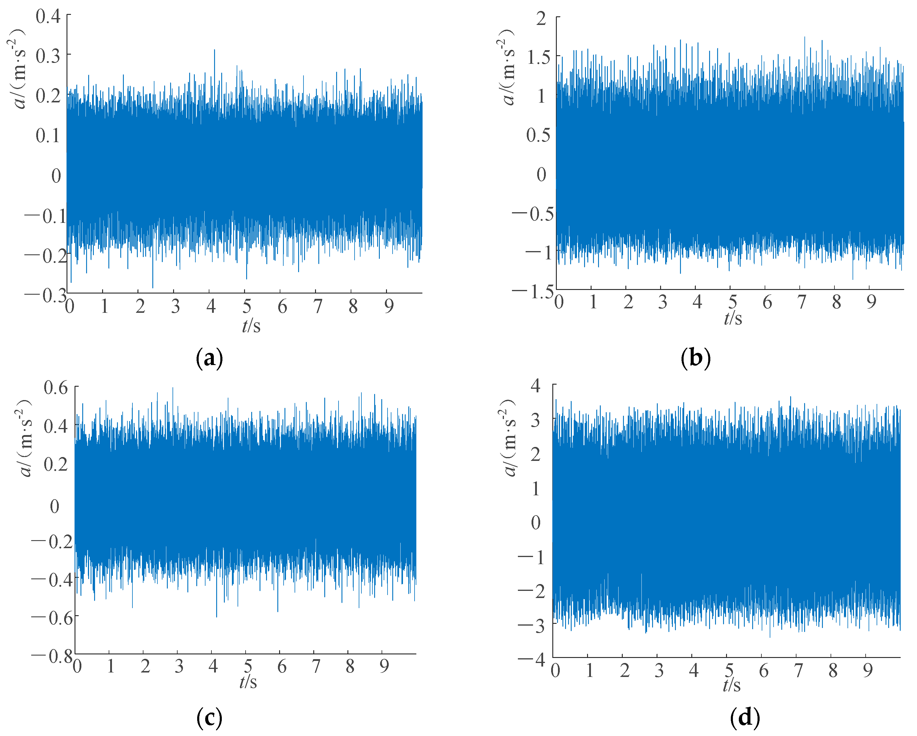
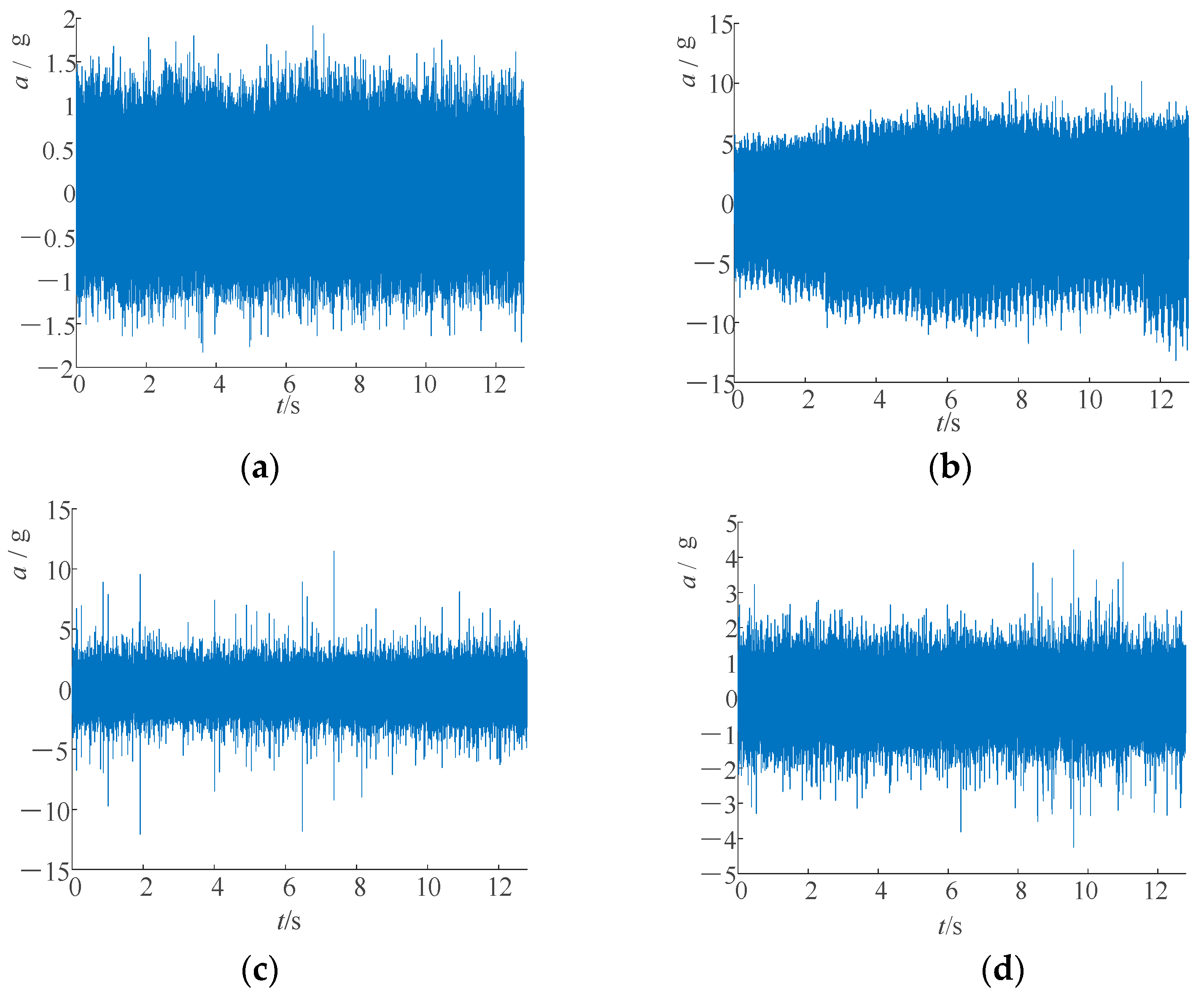
To further validate the relative stability of the pressure signals compared to the vibration signals, a comparison was made with the vibration acceleration signals collected using a vibration accelerometer on the end cap of the axial piston pump. For the three channels of vibration signals collected, it was observed that using the z-direction vibration data yielded better results in the analysis of the signals under abnormal conditions. Figure 16 shows the time domain waveforms of the original vibration signals obtained from the axial piston pump under four distinct working conditions.

Figure 16. Time domain waveform plot of raw vibration signals: (a) normal; (b) swashplate wear; (c) sliding shoe wear; (d) single-plunger loose shoe.

Each sample contained 259 data points obtained using the DTW algorithm for data partitioning. The partitioning of the samples under normal operating conditions resulted in 192 samples with a training-to-testing dataset ratio of 3:1, yielding 144 samples for training and 48 samples for testing. After completing data partitioning for the three abnormal operating states, 48 random samples were selected as the target abnormal samples. The results are presented in Table 6. Anomaly detection was performed using the DTW-RCK-IF composite method and the results were compared with those obtained from the pressure signals, as listed in Table 7.

Table 6. Axial piston pump vibration signal data set partitioning.

Category	Sample Length	Number of Samples	Training Dataset	Testing Dataset	Target Abnormal Samples
normal	259	192	144	48	-
swashplate wear	259	191	0	-	48
sliding shoe wear	259	193	0	-	48
single-plunger loose shoe	259	191	0	-	48

Table 7. Comparison of the detection performance for pressure and vibration signals.

Signal	Vibration Signal			Pressure Signal
	P	R	F1	P	R	F1
normal	100.00	93.75	96.77	100.00	97.56	98.77
swashplate wear	94.12	100.00	96.97	97.62	100.00	98.80
sliding shoe wear	94.12	100.00	96.97	97.62	100.00	98.80
single-plunger loose shoe	94.12	100.00	96.97	97.62	100.00	98.80
average	95.59	98.44	96.92	98.22	99.39	98.79

The results indicate that when vibration signals were used for anomaly detection under four different operating conditions, the average precision was 95.59%, the average recall was 98.44%, and the average F1 score was 96.92%. In comparison, when pressure signals were used for anomaly detection, the average precision increased by 2.63%, the average recall increased by 0.95%, and the average F1 score increased by 1.87%. This suggests that pressure signals are more stable and less susceptible to external factors in many situations. Therefore, the pressure signals yielded superior results for the axial piston pumps when employing the DTW-RCK-IF composite method for anomaly detection on the raw data.

6. Extended Applications of the DTW-RCK-IF Composite Method

To investigate the applicability of the proposed DTW-RCK-IF anomaly detection method, we extended its application to the detection of bearing anomalies. Publicly available datasets offer a wide range of applications and are therefore reliable. Therefore, we used two publicly available datasets to validate the extension and application of the DTW-RCK-IF composite method.

6.1. CWRU Bearing Dataset

This test used bearing data sourced from Case Western Reserve University in the United States [18], and the test platform is illustrated in Figure 17. Damage was induced in the bearings using electrical discharge machining, resulting in deliberate damage to the inner race, rolling elements, and outer race. The collected signals were recorded using an accelerometer. Three types of bearing faults, namely an inner ring fault, rolling element fault, and outer ring fault at the 6 o’clock position, as well as the normal-state data, were selected for validation, with a motor load of 0 hp, speed of 1797 r/min, sampling frequency of 12 kHz, and fault diameter of 0.1778 mm. SKF bearings were used in this study. The first 1.2 × 10⁵ data points of each state were selected. The time domain waveforms of the original signals under the four conditions are shown in Figure 18.

Figure 17. Bearing failure test bench of CWRU.

Figure 18. Bearing vibration signal time domain waveform diagram of CWRU: (a) normal; (b) inner ring fault; (c) rolling element fault; (d) outer ring fault.

In Experiment 1, the DTW-RCK-IF anomaly detection method was extended to practical applications. Using the DTW algorithm for data partitioning, each sample had a length of 801. Under normal operating conditions, the dataset comprised 149 samples with a training-to-testing ratio of 3:1, resulting in 111 samples for training and 38 samples for testing. After completing the data partitioning for the three abnormal operating states, 38 random samples were selected from each target abnormal sample, as listed in Table 8. Subsequently, a CNN with random convolutional kernels was used to extract features from the partitioned data. A total of 1000 one-dimensional random convolutional kernels were employed, generating 2000 feature dimensions that constituted the dataset. Finally, the isolation forest algorithm was used to perform anomaly detection and calculate the performance metrics for the extracted feature dataset. The anomaly detection results are listed in Table 9.

Table 8. CWRU bearing dataset partitioning.

Category	Sample Length	Number of Samples	Training Dataset	Testing Dataset	Target Abnormal Samples
normal	801	149	111	38	-
inner ring fault	801	149	0	-	38
rolling element fault	801	148	0	-	38
outer ring fault	801	149	0	-	38

Table 9. CWRU bearing abnormal test results.

Method	DTW-RCK-IF
	P	R	F1
normal	100.00	98.68	99.34
inner ring fault	98.70	100.00	99.35
rolling element fault	98.70	100.00	99.35
outer ring fault	98.70	100.00	99.35
average	99.03	99.67	99.35

The results demonstrated that the average precision across the four operating conditions was 99.03%, the average recall was 99.67%, and the average F1 score reached 99.35%. This suggests that the DTW-RCK-IF composite method exhibits high applicability to and stability for bearing anomaly detection.

6.2. XJTU-SY Rolling Bearing Dataset

This experiment used a vibration dataset from the rolling–bearing accelerated life test platform XJTU-SY at Xi’an Jiaotong University [19], as shown in Figure 19. The bearing model used was the LDKUER204. Two unidirectional acceleration sensors were installed in the horizontal and vertical directions to capture bearing vibration signals. The sampling frequency was set to 25.6 kHz, with each sampling lasting 1.28 s. The sampling interval was set to 1 min. The experiment was terminated when the amplitude of the vibration acceleration exceeded 10 times the maximum amplitude of the healthy stage. The corresponding degradation data were recorded. In total, data were collected from 15 bearings, including five bearings for each of the three operating conditions. The vibration data in the horizontal direction of the bearing were observed at a speed of 2250 rpm and a radial force of 11 kN. These datapoints included data from the 464th to the 473rd set for the inner ring fault in bearing 2_1, the 59th to the 68th set for the outer ring fault in bearing 2_2, the 138th to the 147th set for the cage fault in bearing 2_3, and the 21st to the 30th set for normal operation in bearing 2_1. The time domain waveforms of the original signals under four operating conditions are shown in Figure 20.

Figure 19. XJTU-SY bearing accelerated life test bench.

Figure 20. Time domain waveform of XJTU-SY bearing vibration signal: (a) normal; (b) inner ring fault; (c) outer ring fault; (d) cage fault.

In Experiment 2, the DTW-RCK-IF anomaly detection method was applied for extended testing. Data were partitioned using the DTW algorithm, resulting in a sample length of 684 data points. Under normal operating conditions, the dataset consisted of 480 samples with a training-to-testing ratio of 3:1, resulting in 360 samples for training and 120 samples for testing. After completing the data partitioning for the three abnormal operating states, 120 random samples were selected from each target abnormal sample, as listed in Table 10. Features were extracted from the partitioned data using a CNN with random convolutional kernels, with 1000 one-dimensional random convolutional kernels used to generate the 2000 feature dimensions that constituted the feature dataset. Finally, the isolation forest algorithm was applied to perform anomaly detection on the feature dataset and calculate the performance metrics. The anomaly detection results are listed in Table 11.

Table 10. XJTU-SY bearing dataset partitioning.

Category	Sample Length	Number of Samples	Training Dataset	Testing Dataset	Target Abnormal Samples
normal	684	480	360	120	-
inner ring fault	684	482	0	-	120
outer ring fault	684	480	0	-	120
cage fault	684	480	0	-	120

Table 11. XJTU-SY bearing abnormal detection results.

Method	DTW-RCK-IF
	P	R	F1
normal	100.00	99.46	99.73
inner ring fault	99.47	100.00	99.73
outer ring fault	99.47	100.00	99.73
cage fault	99.47	100.00	99.73
average	99.60	99.87	99.73

The results indicate that the average precision across the four operating conditions was 99.60%, the average recall was 99.87%, and the average F1 score reached 99.73%. This further underscores the advantages of the proposed DTW-RCK-IF composite method for anomaly detection, demonstrating its strong generality and applicability.

7. Conclusions

An axial piston pump anomaly detection method based on pressure signals is proposed in this paper, namely DTW-RCK-IF. Through a theoretical analysis, modeling simulation tests, and extended application tests, the following conclusions were drawn:

• Compared with the fixed-length partitioning method, the data partitioning and matching approach using the DTW algorithm resulted in higher similarity between the partitioned data.
• Compared with traditional time domain feature extraction and dimensionality reduction methods, a CNN with random convolutional kernel feature extraction can better capture the local features of time series data. This enables the model to learn more effective and comprehensive feature representations, thereby enhancing its generalization capability and robustness.
• Compared with the OCSVM algorithm, the isolation forest anomaly detection method exhibited superior performance in detecting anomalies in large-scale datasets and high-dimensional feature spaces.
• For real-time anomaly detection in axial piston pumps, pressure signals outperform vibration signals. The DTW-RCK-IF composite method can efficiently detect anomalies using only data from normal operating conditions. This demonstrates its sensitivity to abnormal data, thereby yielding effective fault-warning capabilities.
• The DTW-RCK-IF composite method consistently exhibits excellent detection performance when applied to various target objects for anomaly detection, demonstrating its robustness and potential for broad and versatile applications.

However, the method proposed in this study has some inherent limitations. First, it relies on normal-state data for the training of the model. Consequently, in situations with insufficient normal-state data, the performance of the model may be compromised. Second, although the method demonstrates the improved detection of anomalies for certain complex anomaly patterns, additional domain knowledge may be required to design more effective approaches. In summary, this method requires further comprehensive consideration and evaluation based on specific application scenarios and requirements.