Abstract
This work aims to explore some dynamic aspects of the problem of star motion that is impacted by the rotation of the galaxy, which we model as a bisymmetric potential based on a two-dimensional harmonic oscillator with sextic perturbations. We demonstrate analytically that the motion is non-integrable when certain conditions are met. The analytical results for the non-integrability are confirmed by showing the irregularity of the behavior of the motion through utilizing the Poincaré surface of a section as a numerical method. The motion equilibrium positions are detected, and their stability is discussed. We show that the force generated by the rotating frame acts as a stabilizer for the maximum equilibrium points. We display graphically that the size of the stability regions relies on the angular velocity magnitude for the frame. Through the application of Lyapunov’s theorem, periodic solutions can be constructed which are close to the equilibrium positions. Furthermore, we demonstrate that there are one or two families of periodic solutions relying on whether the equilibrium point is a saddle or stable, respectively.
1. Introduction
Galactic dynamics, the study of the movements of galactic masses, is an important branch of astrophysics. It includes the investigations of stars, gases, and dark matter with the goal of understanding the main kinematics features of the three main types of galaxies (elliptical, spiral, and irregular) [1,2,3,4]. The theoretical bases for the subject were established approximately seven decades ago, when the study of dynamics was dominated by integrable and near-integrable systems. The study of galactic motion can be carried out globally. It can also be performed locally near the equilibrium points by using the perturbed oscillators. In the last few decades, several studies on galactic dynamics, mostly focused on elliptical galaxies, were published [5,6,7,8,9,10,11,12], and the existence of periodic solutions and their stability were investigated [13,14,15,16,17,18,19]. El-Sabaa et al. [20] also investigated the bifurcations of the Armbruster–Guckenheimer–Kim (AGK) potential by studying the topological type of the level sets of the integrable cases of the AGK galactic potential. This study was followed by Llibre et al. [21], who analyzed its global dynamics. Except for some studies on stellar orbits, the rotation of galaxies has been ignored in most studies of galactic dynamics [22]. This is in spite of the fact that an elliptical galaxy rotates with a slight angular velocity, and the force produced by the galaxy’s rotation will influence the dynamic (see, for example, [23,24]). This motivates the study of the rotation of a galaxy, modeled by a bisymmetric potential with different perturbations, and the effects of this rotation on the dynamics of star motion. Iñarrea et al. studied the stability of the motion equilibrium positions for a Hénon–Heiles system in a rotating reference frame [25]. Elmandouh in [26] studied the dynamic features of the AGK potential in a rotating reference frame. In that study, he examined the nonintegrability of the system to seek periodic solutions near the equilibrium points. Elmandouh et al. [27] investigated the integrability and stability of equilibria for a quartic galactic potential in a rotating reference frame. Lanchares et al. [28] applied Reeb’s theorem to prove the existence of periodic orbits in a rotating Hénon–Heiles system.
In the present work, we consider the plane motion rotation with a constant angular velocity of a galaxy approximately symmetrical around an axis normal to the plane of rotation. By reversing the normal axis if needed, we may assume that . This motion, similar to that of most elliptical galaxies, is described by a Hamiltonian system that involves a symmetric potential. The Hamiltonian we use is given by
where are the generalized momentum corresponding to the generalized coordinates and U is the four-parameter galactic potential function given by
while , and d are free constants. Recently, Elsabaa et al. [29] studied the existence of periodic solutions and their stability by applying the averaging theorem for the sextic galactic potential while ignoring the rotation of the galaxy. This motivated us to study the influence of the galaxy rotations on some dynamics of the motion which were not considered before in the literature, such as integrability, the stability of the equilibrium positions, and the existence of periodic solutions near the equilibrium positions. The Hamilton canonical equations are
As usual, the dots indicate that the derivative expressed is with respect to time. The equation of the motion (Equation (3)) has a Jacobi integral in the form
where E is an arbitrary constant.
Additionally, the Hamiltonian in Equation (1) physically describes the motion of a particle under the combined action of the potential forces (velocity independent) obtained from the potential in Equation (2) and the gyroscopic forces (velocity-dependent) resulting from the rotation of the reference frame, giving the term .
This work is organized as follows. Section 2 contains the proof of the non-integrability of the Hamiltonian in Equation (1) and shows the behavior of the motion for two different values, leading to regular and irregular behavior of the motion. The equilibrium positions are determined in Section 3. In Section 4, we examine the stability of these equilibrium positions. We show the effect of the rotating reference frame on the stability and linear stability. The periodic solutions near the equilibrium positions are constructed, and the number of periodic solutions is linked to the stability of the equilibrium positions in Section 5.
2. Integrability Analysis
A 2D Hamiltonian system is integrable if it possesses two functionally independent integrals of motion and that are in involution (i.e., ), where represents Poisson brackets [30]. Integrable systems exhibit regularity, enabling the prediction of their behavior for all times. Their explicit solution can be found using quadratures, and they can be used to study non-integrable systems through perturbation theories [31]. The Hamiltonian system in Equation (1) is integrable if it has a complementary integral independent of the Jacobi integral in Equation (4). The problem of finding this integral is complicated due to the fact that its functional form is unknown. Details on constructing integrals of motion are mentioned in [32,33,34,35,36]. On the other hand, there are many methods that prove non-integrability, such as the Yoshida and Morales–Ramis criteria, which are based on the investigation of normal variation equations along a particular solution, and the Ziglin approach, which depends on the examination of the monodromy group associated with a variational equation [37,38,39]. Neither of these techniques work with Hamiltonian systems with linear momentum terms. As a consequence, we rewrote the Hamiltonian in Equation (1) appropriately.
We use the transformation
Then, the Hamiltonian equations (Equation (3)) are transformed into
When tends toward infinity, the non-similarity system in Equation (6) becomes
The system in Equation (7) is a canonical Hamilton equation derived from the Hamiltonian
We will study the non-integrability of the system in Equation (8) and show that the non-integrability of the Hamiltonian implies the non-integrability of the Hamiltonian H in Equation (1):
Theorem 1.
If the Hamiltonian is non-integrable, then the Hamiltonian H is non-integrable.
Proof.
If the Hamiltonian H is integrable, then it has a complementary integral independent of the Jacobi integral in Equation (4). By applying the transformation in Equation (5) to the complementary integral and taking the limit as tending toward infinity, we obtain a complementary integral for , confirming the integrability of . The non-integrability of H follows by contradiction. □
Yoshida introduced a non-integrability theorem based on Ziglin’s analysis [37]. This theorem deals only with homogeneous potentials:
Theorem 2.
(Yoshida’s theorem) Let be a Hamiltonian system with homogeneous potential of a degree . Then, it is non-integrable if
where
is the non-integrability coefficient and is the solution of the algebraic equation .
We are going to apply Theorem 2 to investigate the non-integrability of the Hamiltonian , which is given by Equation (8). The potential is
The solutions to the algebraic equation are as follows:
- (1)
- , where ;
- (2)
- , where .
For the first solution, the non-integrability coefficient is , while the non-integrability coefficient corresponding to the second solution is . Taking into account Yoshida’s theorem (Theorem 2), the Hamiltonian in Equation (8) is non-integrable if at least one of the following conditions is satisfied:
The next Theorem follows from Theorem 1 and Theorem 2:
Theorem 3.
Remark 1.
Theorem 3 provides the sufficient conditions for non-integrability. This means that if one of the conditions in Equation (2) is fulfilled, then the Hamiltonian in Equation (1) is non-integrable, and no further investigation is required. On the other hand, if neither conditions in Equation (2) hold, then the Hamiltonian in Equation (1) may be either integrable or non-integrable. In such a case, verifying integrability requires finding an additional integral functionally independent of the Jacobi integral in Equation (4).
It is worth motioning that Elmandouh introduced a theorem [34] based on studying the solvability of the differential Galois group associated with the normal variational equation, which can be applied effectively to give the necessary conditions for integrability and sufficient conditions for the non-integrability for a wide class of non-homogeneous potentials, including the galactic potential in Equation (2) as a special case.
Special cases:
- (1)
- If , then the Hamiltonian in Equation (1) takes the form below in polar coordinates :
The Hamiltonian in Equation (13) is integrable since it has two independent first integrals of the motion. The first is the momentum corresponding to the cyclic coordinate , with the second being the Jacobi integral, which takes the form
It should be noted that the constants , and d in the present case do not satisfy Theorem 3 since does not fall in the non-integrability regions.
- (2)
- If and , then the Hamiltonian in Equation (1) is separable into Cartesian coordinates. As a result of the separability of the Hamiltonian, the additional integral is quadratic in momentum. The integrals of the motion for this case are
We present the Poincaré surface of a section for the Hamiltonian in Equation (1) with the potential function in Equation (2) when the parameters , d, and take two different values. One of them satisfies Theorem 3, and the other does not agree with it. When , and is arbitrary, the non-integrability coefficient is outside the non-integrability region. The Poincaré surface of the section, which is illustrated by Figure 1a, seems to be regular and gives some indications about the integrability of the problem. This indication is confirmed by finding the complete set of the first integrals of the motion, in which one of them is a cyclic integral in polar coordinates . If , and is free, then Theorem (3) is met, and consequently, the Hamiltonian in Equation (1) is non-integrable. The Poincaré surface of the section corresponding to this case is irregular, which is usual for the non-integrability of the Hamiltonian in Equation (1). Hence, both the numerical and analytical results agree, and this shows the correctness of the obtained analytical results.
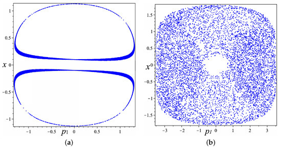
Figure 1.
Poincaré surface of section for the Hamiltonian in Equation (18) with a cross section plane on the Jacobi integral level, where (a) and (b) .
3. Equilibria
The equilibria of the system in Equation (3) can be obtained by setting the left-hand sides (the derivatives) in the Hamiltonian equations equal to zero to obtain
Rather than referring to the equilibrium positions as , we indicate them as , since can be directly evaluated by Equation (16a). By solving Equations (17a) and (17b), the equilibria are obtained in the next theorem:
Theorem 4.
The Hamiltonian system in Equation (3), corresponding to the Hamiltonian in Equation (1), has the following as equilibrium positions:
- 1.
- If , or if , then is the only equilibrium point;
- 2.
- If , then there is an equilibrium point ;
- 3.
- If , then there is an equilibrium point ;
- 4.
- If such that , then there is an equilibrium point .
It should be mentioned that there are some limiting cases in which either a, b, or approaches zero, taking into account the equilibrium position existence condition. For example, if , then blows up to infinity through the positive Y axis, while blows up to infinity through the negative Y axis. The same applies to the equilibrium positions via the positive and negative X axes. If the conditions in item 4 are satisfied, then equilibrium positions blow up to infinity through the line if the coordinates of the equilibrium point have the same sign or through the line if the coordinates have a distinct sign. Moreover, if , then the analysis of the dynamics reduces to that of a linear system which is readily understood. Dynamic analysis is more subtle if the constants are not zero simultaneously, as the nonlinear terms alter the behavior of the system.
4. Stability Analysis
First, we apply the Lagrange theorem [40], which has the advantage of yielding some information about the trapping and escape dynamics. To be a self-contained article, we recall the Lagrange theorem:
Theorem 5.
(Lagrange theorem) [40] For a conservative system, if the potential energy has a strict minimum at some positions, then these positions are the positions of stable equilibrium points.
4.1. Application of the Lagrange Theorem
To apply the Lagrange Theorem 5, it is essential to find the effective potential of the problem. This requires a re-expression of the Hamiltonian in Equation (1) in terms of the generalized velocities rather than the generalized momentum. Using the equations in Equation (3), we obtain
where is the effective potential given by
Notice that when , the effective potential and potential in Equation (2) are identical. Since the system of equations is the same as in Equation (17), the equilibrium positions of the Hamiltonian system in Equation (1) are the critical points of the effective potential (Equation (19)). The nature of these positions is determined in Theorem 6 below by examining the Hessian matrix for the effective potential and using the Lagrange theorem. The following remark is needed:
Remark 2.
If A is a non-singular matrix, then the matrix A is positive definite if and only if . The matrix A is negative definite if and only if .
Theorem 6.
Under the existence conditions for the equilibrium points in Theorem 4, the following are satisfied:
- 1.
- The equilibrium is stable if . If , then is an unstable maximum critical point;
- 2.
- The equilibrium is unstable when . If , then is a stable position. If and , then the point is unstable and maximally critical;
- 3.
- The equilibrium is unstable when . If , then is a stable position. The positions are maximally unstable if and ;
- 4.
- The equilibrium is unstable when . The case where implies that the point is stable if . The positions are unstable and maximally critical if and .
Proof.
The Hessian matrix for the effective potential in Equation (19) takes the form
We examine the Hessian matrix at the equilibrium positions calculated in Theorem 4. For , the Hessian matrix in Equation (20) takes the form
with . Using Remark 2, the point is either a local minimum if or local maximum if . Based on the Lagrange theorem, is stable if and unstable if . The Hessian matrix in Equation (20) at is
whose determinant is and whose trace is . This implies the following:
- If , then is an indefinite matrix, and the point is a saddle and hence unstable.
- If , the point is a local minimum and hence stable if . If , then it is a local maximum and hence unstable.
Similarly, the case for with replacing . For the equilibrium point , the Hessian matrix (Equation (20)) is
where the off-diagonal entries have the same sign. The determinant of is . If , then the equilibrium point is a saddle and hence unstable. If , then we check the sign of the trace which follows the sign of . If , then the point is a local minimum and hence stable. If , then the case where and are both negative gives as a local maximum and is thus unstable. The case where both and are positive and leads to a contradiction, so it never happens. □
It should be noticed that in all the above cases, the Hessian matrix becomes null when and no information about the equilibrium positions can be derived. Consequently, we exclude the case where from further discussion, as it demands a special investigation outside the scope of this work.
Notice that the degree of instability for the maximum equilibrium points is two, and according to Lord Kelvin’s proposition [41], with the addition of gyroscopic forces, these positions remain stable when they are the minimum for the effective potential in Equation (19), while the unstable maximum equilibrium points for the effective potential can be stabilized by the forces resulting from the rotating frame (gyroscopic forces). Consequently, we must apply the linear approximation for the stability of these positions [40]:
4.2. Linear Stability
This section completes the study in Section 4.1 by investigating the linear stability of the equilibrium positions given in Theorem 4. The linearization system corresponding to the Hamiltonian system in Equation (3) takes the form
where are the perturbed variables for , and , respectively. The matrix is the Jacobian matrix evaluated at the equilibrium position given by
where , and . The eigenvalues of the Jacobian matrix in Equation (25) are the roots of the characteristic equation
where M and N are given by
The equilibrium position is linearly stable if the zeros of the characteristic equation (eigenvalues of the Jacobian matrix in Equation (25)) have pure imaginary roots, and the Jacobian matrix is semi-simple. Thus, the conditions for linear stability are
It is worth mentioning that if at least one of the conditions in Equation (28) is not satisfied at , then the equilibrium position is unstable, and the problem does not require further investigation. Based on the Lyapunov theorem (see, for example, [41]), the instability of the equilibrium position in a linear approximation is still valid when the nonlinear terms in the Hamilton system in Equation (3) are considered, while the stability of the equilibrium position is not necessarily still valid when the nonlinear terms are taken into account. This means the linear approximation analysis gives the necessary conditions for stability and sufficient conditions for instability.
According to Theorem 6, the equilibrium point is a maximum critical point for the effective potential in Equation (19) if and the eigenvalues of the Jacobian matrix are and . Hence, is a linearly stable maximum. This proves the first statement in the following theorem:
Theorem 7.
For the equilibrium positions of the Hamiltonian system (3), we have
- 1.
- If all the coefficients and , then is a linearly stable maximum.
- 2.
- Assuming , the positions are linearly stable maximums if and . Otherwise, they are Lyapunov unstable.
- 3.
- Assuming , the positions are linearly stable maximums if and . Otherwise, they are Lyapunov unstable.
where .
Proof.
By Theorem 6, the equilibrium positions are the maximums for the effective potential in Equation (19) if . To maintain the equilibrium condition, since , b must be negative, then . Let . By calculating the expressions for M and N at the equilibrium positions , we have
The equilibrium positions are linearly stable if the conditions in Equation (28) are satisfied, taking into account the existence of the condition . The two conditions and are satisfied together if
To guarantee the correctness of the last inequality, we find the possible values of such that is verified. Thus, we have . Let and .
Direct calculations show that for all , and
Thus, the polynomial has a unique root in the interval I. Hence, the equilibrium position is a linearly stable maximum if
Analogous procedures can be applied to investigate the linear stability of the equilibrium position . □
The regions of linear stability of the equilibrium point are delimited by the two straight lines and , where is the slope of the second line as well as the region in which the equilibrium positions are the maximums, as determined by the two lines . Hence, the size of the region of linear stability relies on the value of the angular velocity . Figure 2 outlines the zone of linear stability in yellow, which grows as the value of the angular velocity increases, and it reaches the maximum size when (i.e., it covers all the regions of the maximum positions in gray for ). This means the force resulting from the rotating frame controls the regions of stability and instability. On another side, if at least one condition in Equation (31) is not fulfilled, then the equilibrium position becomes Lyapunov unstable. The same discussion and similar graphs can be constructed for the equilibrium point using instead of .
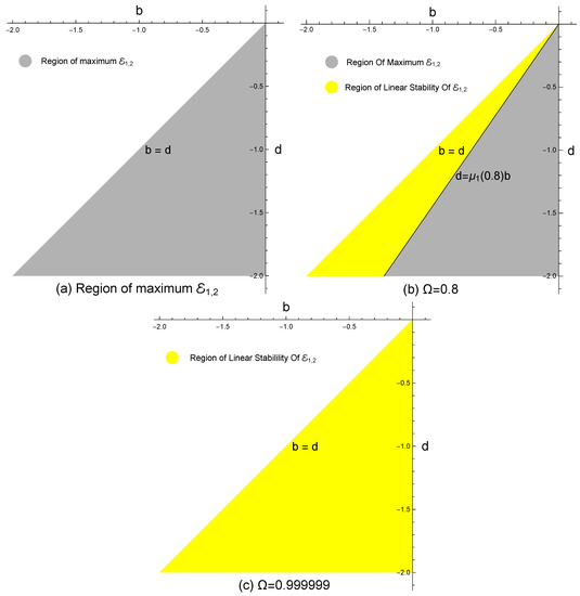
Figure 2.
Regions of stability and instability for the equilibrium position in the plan of the parameters .
According to Theorem 6, the equilibrium positions are the maximums for the effective potential in Equation (19) if and . The following theorem shows the conditions for their linear stability, taking into account the existence condition .
Theorem 8.
Assuming , the equilibrium positions of the Hamiltonian system in Equation (3) are linearly stable maximums if and , where
Proof.
Considering the equilibrium condition , the quantities and are both positive or both negative. Therefore, the equilibrium positions are the maximums for the effective potential in Equation (19) if all the quantities , and are negatives (the case where and are both positive and is negative will lead to a contradiction and never happen). To verify the linear stability of , we compute the corresponding M and N in Equation (27) to obtain
Note that N is positive. To check the signs of the other quantities, let . Since , then , and it easily follows that :
- To find the conditions for , we write as a function in the two variables and to obtainFor each fixed , the sign of is determined by the sign ofSince the discriminate of is , there are two different roots for , given byIt is easy to verify that for , where at . For each fixed such that , the function is , and hence is non-negative on and negative on . Therefore, we have to exclude the interval from the possible values of .
- On the interval , we investigate the sign of M. By writing M as a function in the two variables and , we obtainFor each , all the quantities , and are positive, and the map is decreasing on . For a fixed , the quantity if and only if . Direct computations show the following:
- –
- At the fixed value , we have for all . Therefore, for each and , we have , and then . Therefore, we must also exclude the interval from the possible values for .
- –
- At the fixed value , we have for each . Therefore, for each and , we have , and then . The case where yields and must be excluded.
- –
- At the fixed point , we have for . Therefore, for each and , we have , and then . Therefore, we must also exclude the interval from the possible values of . Note that even though is not included in the interval under consideration, is continuous at , so we can study the relation between and when tends toward 1.
Therefore, all the three quantities are non-negative if and .
□
The zone of linear stability for the motion equilibrium positions is specified by the two lines and , displayed in yellow in Figure 3, as well as the zone in which these positions are the maximums, which are limited by the lines and , as clarified in yellow in Figure 3. The size of the linear stability relies on the value of the angular velocity . As shown in Figure 3b,c, the region of linear stability grows as the angular velocity tends toward one, and at the same time, the size of the Lyapunov instability decreases. Moreover, when tends toward one, the linear stability covers the regions in which are the maximums. Hence, the force resulting from the rotating reference frame can be used as a stabilizer for the unstable maximum equilibrium points.
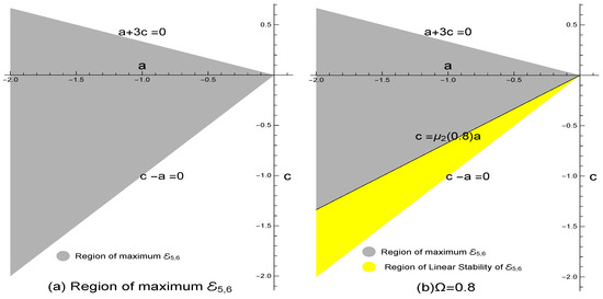
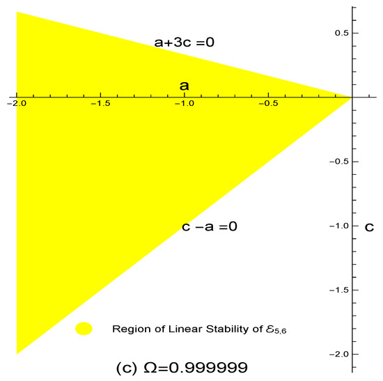
Figure 3.
Regions of stability and instability for the equilibrium position on the plane of the parameters c and a.
5. Periodic Motion
In this section, periodic solutions for the Hamiltonian system in Equation (3) around its equilibrium positions are discussed based on the Lyapunov theorem [42], which has been successfully applied in several works. Yehia [43] presented the periodic solutions near the equilibrium position for mechanical systems in general, while El-Sabaa introduced periodic solutions for the motion of a rigid body’s dynamics in a central Newtonian field [44]. Elmandouh [26] found periodic solutions for the AGK potential nearest to its equilibrium points. El-Sabaa et al. [29] constructed periodic solutions for the sextic galactic potential in a non-rotating reference frame.
The Lagrangian equations of the motions are
where V is given by Equation (19). The equations of the motion in Equation (34) has a first integral
where E is an arbitrary constant. This integral is called the Jacobi integral. Since the equilibrium point is a critical point for the effective potential V, we have
where denotes the Jacobi integral value at the point . To describe the perturbed motion about , we introduce
where p and q are perturbation variables. Notice that the expressions in Equation (37) transform the equilibrium point to the origin of the coordinates. When inserting the expressions in Equation (37) into the equations of motion (34), we have
Using a new variable instead of the time through the time transformation yields
where is a free parameter. By applying the transformation in Equation (39), the system in Equation (38) is converted into
where refers to the derivative with respect to . Following the Lyapunov theorem [42], we assume the periodic solutions as a power series of n which, in our case, depends on the Jacobi integral value (i.e., it depends on E). Assume that
where are constants and and are periodic functions of t with a period that can be written as
By substituting the expressions in Equations (41) and (42) into Equation (40) and finding the first order approximation, we have
Our goal is accomplished by looking for solutions to Equation (43) in the form of
where are the free constants that need to be determined. When putting the expressions in Equation (44) into Equation (43), we obtain
where and are arbitrary constants introduced instead of the old ones for the suitability, while is the frequency, and it takes the value
where is given by
Based on the values , and , there are single or double values of the frequency . Let us clarify this point:
- If , this means is an extreme point for the effective potential in Equation (19). Thus, we have two frequencies if the conditionis verified. This condition is always satisfied when is the minimum value of the effective potential. Thus, there are two values for the frequency. Consequently, there are two periodic families of orbits depending on the parameter n about the stable minimum point of the effective potential.
- If , then the point is a saddle point for the effective potential in Equation (19). There is a unique value for the frequency which is obtained from Equation (46), which takes the positive sign. Hence, there is exactly one periodic orbit around the saddle point for the equilibrium point.
We outlined the obtained results graphically by introducing certain values for the included parameters. The equilibrium point is a stable minimum critical point for the effective potential in Equation (19) if we select , and . For these values, Equation (46) gives two real frequencies: and . Thus, there are two periodic orbits close to the equilibrium point , as outlined in Figure 4a. For the equilibrium point , we choose , which guarantees the existence of this equilibrium alongside . There are two possible choices for the parameter d:


Figure 4.
Periodic solutions close to the equilibrium points and . The green solid circle indicates the equilibrium position.
Figure 4.
Periodic solutions close to the equilibrium points and . The green solid circle indicates the equilibrium position.


6. Discussion
This work explored some aspects of motion under the sextic galactic potential. More specifically, we studied the influence of the forces resulting from a rotating reference frame on the dynamics. The non-integrability of the problem was examined using Yoshida’s analysis. This analysis applies only to the homogeneous potential, so we applied certain similar transformations to convert the original non-homogeneous potential to a homogeneous one. We also used a Poincare surface section as a numerical tool to confirm the obtained analytical results for two values of the parameters: one satisfying the non-integrability Theorem 3 and the other not satisfying it. The stability of the equilibrium position was investigated by applying the Lagrange theorem (Theorem 5), which implies the stability of the minimum positions and the instability of the maximum positions of the effective potentials. As a result, the degree of instability of the maximum equilibrium positions was two. The gyroscopic forces, which resemble the forces resulting from the rotating reference frame, can be utilized as a stabilizer for these unstable positions. Therefore, we applied the linear approximation method, which was also employed to illustrate the dependence of the linear stability regions on the angular velocity. Some figures in the plane of the parameters were used to describe the dependence of the stability zones on the angular velocity. The Lyapunov theorem has been applied to construct periodic solutions that are almost close to the equilibrium positions. We also proved that near the stable equilibrium positions, there are two periodic families as well as one periodic family of orbits near the unstable equilibrium positions.
Author Contributions
Conceptualization, A.E. and M.A.N.; methodology, A.E.; software, M.A. and A.E.; validation, M.A.N., A.E., and M.A.; formal analysis, M.A.; investigation, M.A.; resources, A.E. and M.A.N.; data curation, M.A.N.; writing original draft preparation, A.E. and M.A.; writing—review and editing, M.A.N. and A.E.; visualization, A.E.; supervision, A.E. and M.A.N.; project administration, A.E.; funding acquisition, M.A. All authors have read and agreed to the published version of the manuscript.
Funding
This work was supported by the Deanship of Scientific Research, Vice Presidency for Graduate Studies and Scientific Research of King Faisal University in Saudi Arabia (Grant No. GRANT2118).
Data Availability Statement
Not applicable.
Acknowledgments
The authors would like to acknowledge the support from King Faisal University in Saudi Arabia (Grant No. GRANT2118).
Conflicts of Interest
The authors declare no conflict of interest.
References
- Contopoulos, G. Order and Chaos in Dynamical Systems. Milan J. Math. 2009, 77, 101. [Google Scholar] [CrossRef]
- Arnold, V.; Kozlov, V.; Neishtadt, A. Dynamical system III. In Mathematical Aspects of Classical and Celestial Mechanics; Springer: Berlin/Heidelberg, Germany, 2006. [Google Scholar]
- Ignacio, F. Fundamentals of Galaxy Dynamics, Formation and Evolution; UCL Press: London, UK, 2019. [Google Scholar]
- Rastorguev, A.; Utkin, N.; Zabolotskikh, M.; Dambis, A.; Bajkova, A.; Bobylev, V. Galactic masers: Kinematics, spiral structure and the disk dynamic state. Astrophys. Bull. 2017, 72, 122–140. [Google Scholar] [CrossRef]
- Caranicolas, N. A mapping for the study of the 1:1 resonance in a galactic type Hamiltonian. Celest. Mech. Dyn. Astron. 1989, 47, 87–96. [Google Scholar] [CrossRef]
- Caranicolas, N. Exact periodic orbits and chaos in polynomial potentials. Astrophys. Space Sci. 1990, 167, 305–313. [Google Scholar]
- Caranicolas, N. Global stochastically in a time-dependent galactic model. Astron. Astrophys. 1990, 227, 54–60. [Google Scholar]
- Caranicolas, N.; Innanen, K. Chaos in a galaxy model with nucleus and bulge components. Astron. J. 1991, 102, 1343–1347. [Google Scholar] [CrossRef]
- Karanis, G.; Caranicolas, N. Transition from regular motion to chaos in a logarithmic potential. Astron. Astrophys. 2001, 367, 443–448. [Google Scholar] [CrossRef]
- Habib, S.; Kandrup, H.; Mehon, M. Chaos and noise in galactic potentials. Astron. J. 1997, 480, 155–166. [Google Scholar] [CrossRef]
- Llibre, J.; Valls, C. On the analytic integrability of the cored galactic Hamiltonian. Appl. Math. Lett. 2014, 33, 35–39. [Google Scholar] [CrossRef]
- Bajkova1, A.; Smirnov1, A.; Bobylev1, V. Study of the Influence of an Evolving Galactic Potential on the Orbital Properties of 152 Globular Clusters with Data from the Gaia EDR3 Catalogue. Astron. Lett. 2021, 47, 454–473. [Google Scholar] [CrossRef]
- Alfaro, F.; Llibre, J.; Pérez-Chavela, E. Periodic orbits for a class of galactic potentials. Astrophys. Space Sci. 2013, 344, 39–44. [Google Scholar] [CrossRef]
- Llibre, J. Averaging theory and limit cycles for quadratic systems. Rad. Math. 2002, 11, 215–228. [Google Scholar]
- Llibre, J.; Makhlouf, A. Periodic orbits of the generalized Friedmann- Robertson-Walker Hamiltonian systems. Astrophys. Space Sci. 2013, 344, 45–50. [Google Scholar] [CrossRef]
- Llibre, J.; Roberto, L. Periodic orbits and non-integrability of Armbruster-Guckenheimer-Kim potential. Astrophys. Space Sci. 2013, 344, 69–74. [Google Scholar] [CrossRef]
- Llibre, J.; Vidal, C. Periodic orbits and non-integrability in a cosmological scalar field. J. Math. Phys. 2012, 53. [Google Scholar] [CrossRef]
- Llibre, J.; Vidal, C. New 1:1:1 periodic solution in 3-dimensional galactic-type Hamiltonian systems. Nonlinear Dyn. 2014, 78, 968–980. [Google Scholar] [CrossRef]
- Llibre, J.; Pa¸sca, D.; Valls, C. Periodic solutions of a galactic potential. Chaos Solitons Fractals 2014, 61, 38–43. [Google Scholar] [CrossRef]
- El-Sabaa, F.; Hosny, M.; Zakria, S. Bifurcations of Armbruster Guckenheimer Kim galactic potential. Astrophys. Space Sci. 2019, 364, 1–9. [Google Scholar] [CrossRef]
- Llibre, J.; Valls, C. Global dynamics of the integrable Armbruster-Guckenheimer-Kim galactic potential. Astrophys. Space Sci. 2019, 364, 1–6. [Google Scholar] [CrossRef]
- De Zeeuw, T.; Merritt, D. Stellar orbits in a triaxial galaxy. I-Orbits in the plane of rotation. Astrophys. J. 1983, 267, 571–595. [Google Scholar] [CrossRef]
- Bertola, F.; Capaccioli, M. Dynamics of early type galaxies. I-The rotation curve of the elliptical galaxy NGC 4697. Astrophys. J. 1975, 200, 439–445. [Google Scholar] [CrossRef]
- Caranicolas, N.; Barbanis, B. Periodic orbits in nearly axisymmetric stellar systems. Astron. Astrophys. 1982, 114, 360–366. [Google Scholar]
- Iñarrea, M.; Lanchares, V.; Palacián, J.F.; Pascual, A.I.; Salas, J.P.; Yanguas, P. Lyapunov stability for a generalized Hénon–Heiles system in a rotating reference frame. Appl. Math. Comput. 2015, 253, 159–171. [Google Scholar] [CrossRef]
- Elmandouh, A. On the dynamics of Armbruster Guckenheimer Kim galactic potential in a rotating reference frame. Astrophys. Space Sci. 2016, 361, 1–12. [Google Scholar] [CrossRef]
- Elmandouh, A.; Ibrahim, A. Non-integrability, stability and periodic solutions for a quartic galactic potential in a rotating reference frame. Astrophys. Space Sci. 2020, 365, 1–11. [Google Scholar] [CrossRef]
- Lanchares, V.; Pascual, A.I.; Iñarrea, M.; Salas, J.P.; Palacián, J.; Yanguas, P. Reeb’s theorem and periodic orbits for a rotating Hénon–Heiles potential. J. Dyn. Differ. Equa. 2021, 33, 445–461. [Google Scholar] [CrossRef]
- El-Sabaa, F.; Amer, T.; Gad, H.; Bek, M. Existence of periodic solutions and their stability for a sextic galactic potential function. Astrophys. Space Sci. 2021, 366, 1–11. [Google Scholar] [CrossRef]
- Abraham, R.; Marsden, J.E. Foundations of Mechanics; Number 364; American Mathematical Soc.: Providence, RI, USA, 2008. [Google Scholar]
- Tabor, M. Chaos and Integrability in Nonlinear Dynamics: An Introduction; Wiley Interscience: Hoboken, NJ, USA, 1989. [Google Scholar]
- Elmandouh, A. New integrable problems in a rigid body dynamics with cubic integral in velocities. Results Phys. 2018, 8, 559–568. [Google Scholar] [CrossRef]
- Elmandouh, A. First integrals of motion for two dimensional weight-homogeneous Hamiltonian systems in curved spaces. Commun. Nonlinear Sci. Numer. Simul. 2019, 75, 220–235. [Google Scholar] [CrossRef]
- Elmandouh, A. On the integrability of new examples of two-dimensional Hamiltonian systems in curved spaces. Commun. Nonlinear Sci. Numer. Simul. 2020, 90, 105368. [Google Scholar] [CrossRef]
- Szumiński, W. On certain integrable and superintegrable weight-homogeneous Hamiltonian systems. Commun. Nonlinear Sci. Numer. Simul. 2019, 67, 600–616. [Google Scholar] [CrossRef]
- Yehia, H.; Elmandouh, A. A new conditional integrable case in the dynamics of a rigid body-gyrostat. Mech. Res. Commun. 2016, 78, 25–27. [Google Scholar] [CrossRef]
- Yoshida, H. A criterion for the non-existence of an additional integral in Hamiltonian systems with a homogeneous potential. Phys. D Nonlinear Phenom. 1987, 29, 128–142. [Google Scholar] [CrossRef]
- Yoshida, H. A criterion for the non-existence of an additional analytic integral in Hamiltonian systems with n degrees of freedom. Phys. Lett. A 1989, 141, 108–112. [Google Scholar] [CrossRef]
- Ziglin, S.L. Branching of solutions and nonexistence of first integrals in Hamiltonian mechanics. I. Funktsional’nyi Analiz i ego Prilozheniya 1982, 16, 30–41. [Google Scholar] [CrossRef]
- Gantmacher, F. Lectures in Analytical Mechanics; Mir Publishers: Moscow, Russia, 1970. [Google Scholar]
- Chetayev, N.; Nadler, M.; Babister, A.; Burlak, J.; Teichmann, T. The stability of motion. Phys. Today 1962, 15, 70. [Google Scholar] [CrossRef]
- Liapunov, A. The General Problem of the Stability of Motion. Int. J. Control 1992, 55, 531–534. [Google Scholar] [CrossRef]
- Yehia, M. On periodic, almost stationary motions of a rigid body about a fixed point: PMM vol. 41, n≗ 3, 1977, pp. 556–558. J. Appl. Math. Mech. 1977, 41, 571–573. [Google Scholar]
- El-Sabaa, F. About the periodic solutions of a rigid body in a central Newtonian field. Celest. Mech. Dyn. Astron. 1993, 55, 323–330. [Google Scholar] [CrossRef]


Disclaimer/Publisher’s Note: The statements, opinions and data contained in all publications are solely those of the individual author(s) and contributor(s) and not of MDPI and/or the editor(s). MDPI and/or the editor(s) disclaim responsibility for any injury to people or property resulting from any ideas, methods, instructions or products referred to in the content. |
© 2023 by the authors. Licensee MDPI, Basel, Switzerland. This article is an open access article distributed under the terms and conditions of the Creative Commons Attribution (CC BY) license (https://creativecommons.org/licenses/by/4.0/).