A Novel Remaining Useful Life Probability Prediction Approach for Aero-Engine with Improved Bayesian Uncertainty Estimation Based on Degradation Data

Abstract

As the heart of aircraft, the aero-engine is not only the main power source for aircraft flight but also an essential guarantee for the safe flight of aircraft. Therefore, it is of great significance to find effective methods for remaining useful life (RUL) prediction for aero-engines in order to avoid accidents and reduce maintenance costs. With the development of deep learning, data-driven approaches show great potential in dealing with the above problem. Although many attempts have been made, few works consider the error of the point prediction result caused by uncertainties. In this paper, we propose a novel RUL probability prediction approach for aero-engines with prediction uncertainties fully considered. Before forecasting, a principal component analysis (PCA) is first utilized to cut down the dimension of sensor data and extract the correlation between multivariate data to reduce the network computation. Then, a multi-layer bidirectional gate recurrent unit (BiGRU) is constructed to predict the RUL of the aero-engine, while prediction uncertainties are quantized by the improved variational Bayesian inference (IVBI) with a Gaussian mixture distribution. The proposed method can give not only the point prediction of RUL but also the confidence interval of the prediction result, which is very helpful for real-world applications. Finally, the experimental study illustrates that the proposed method is feasible and superior to several other comparative models.

1. Introduction

With the vigorous development of the aviation industry, aircraft are widely used in many fields, such as civil, military, transportation, and other fields. The aero-engine is the core component of aircraft that provides the main flight power for aircraft [1,2]. Aero-engines usually work continuously in a high-temperature, high-pressure, dusty environment, so their health state deteriorates with long-term operation. As such, it is of great importance to establish a comprehensive prognostics health management (PHM) system for aero-engines [3,4,5,6]. PHM includes fault detection and isolation, fault diagnosis, remaining useful life (RUL) prediction and health management [7,8], etc. PHM is becoming an important part of the design and use of new-generation aircraft, ships, vehicles, and other systems. RUL prediction is one of the main tasks for PHM that has been researched by many scholars in the past decades.

The existing RUL prediction methods can be divided into physical model-based methods, statistical data model-based methods, machine learning model-based methods, and hybrid model-based methods. Physical model-based prediction methods require a deep understanding of system structures and precise analysis of failure mechanisms in order to establish a reliable degradation model for RUL prediction [9,10]. However, the system structures are complex and surrounding conditions changeable, it is next to impossible to build a universal degradation model with sufficient accuracy in practical applications. The statistical data model-based methods fit historical data with a random relationship model or stochastic process model to obtain the RUL prediction [11,12]. Though such methods consider the impact of system uncertainty on RUL, they are unable to mine the internal, complex, in-depth features of the monitoring data and, thus, cannot make sufficient utilization of massive monitoring data. The primary advantage of machine learning model-based methods is that they do not require a priori information about system degradation while making use of complex relationships in the monitoring data [13,14]. The hybrid model-based methods are achieved by combining the advantages of different models [15], but they often require a more complex structure than a single model. Against the backdrop of more and more massive data that we can obtain, machine learning model-based methods have definitely become the mainstream direction.

Deep learning-based methods are representative of machine learning model-based methods [16,17,18]. In recent years, deep learning has been successfully applied to deal with the RUL prediction problem of aero-engines due to its strong ability in nonlinear modeling. For example, a multi-objective deep belief network ensemble (MODBNE) method was proposed in [19]. It could extract features automatically and estimate the RUL of an aero-engine by building multiple deep belief networks (DBNs). The convolutional neural network (CNN) is also welcomed by many scholars because of its unique advantages in feature extraction. In ref. [20], Li et al. constructed a new deep convolutional neural network approach, which could predict the RUL of an aero-engine by learning features of the originally collected sensor data without accurate physical or expert knowledge. Considering the high-dimensional characteristics and complexity of aero-engine monitor data, Liu et al. [21] adopted deep convolutional neural networks to extract information from the input data and then used a strong classifier-light gradient boosting machine (LightGBM) to replace the fully connected layer of deep convolutional neural networks to improve the accuracy of RUL prediction. Kim et al. [22] proposed a convolutional neural network-based multi-task learning method for RUL prediction considering the influence of the health status detection process on RUL estimation.

Unfortunately, the CNN-based methods mentioned above lack time memory ability. As such, these methods cannot extract the temporal dependence in the degradation data. In recent years, approaches based on the recurrent neural network (RNN) and its variants have become dominant in RUL prediction. In ref. [23], Liu et al. presented an improved multi-stage long short-term memory network with a clustering method for the RUL prediction of aero-engines, which integrated clustering analysis and long short-term memory (LSTM) to improve the low prediction accuracy of traditional single-parameter and single-stage models. Xia et al. [24] researched an LSTM method with a multi-layer self-attention (MLSA) mechanism for aero-engine RUL estimation. The degradation data characteristics and time step characteristics were extracted simultaneously by the MLSA mechanism, where LSTM was used to capture the degradation process of the system. To suppress the raw signal noise and improve the quality of input data, Jin et al. [25] provided a novel bidirectional LSTM-based two-stream network. One stream came from the raw data and the other from a series of new handcrafted feature flows (HFFs). Then, bidirectional LSTM (BiLSTM) was used to estimate the RUL of aero-engines based on these processed data. Moreover, Li et al. [26] constructed an integrated deep multiscale feature fusion network (IDMFFN) for aero-engine RUL prediction. Different scale features were firstly extracted by convolutional filters with different sizes, and then a gate recurrent unit (GRU) layer was built to replace the traditional, fully connected layer to obtain more accurate prediction results. Song et al. [27] put forward a hierarchical scheme with LSTM networks to regard RUL prediction as a bi-level optimization problem; the lower level was used to predict the time series in the near future, and the upper level was used to estimate the RUL by merging the measurement data and the predicted ones obtained by the lower level.

Despite the advancement of the above deep learning models, most of them only provide point values of RUL and neglect the prediction uncertainties. In reality, RUL prediction is often impacted by many uncertain factors including data uncertainty imported by noise from the data themselves or the measurement errors of the sensors, changes in operating conditions (also called aleatoric uncertainty) [28,29], and model uncertainty introduced by limited access to monitoring data (also called epistemic uncertainty) [30,31]. Therefore, it is necessary to analyze these uncertainties in deep learning to avoid making incorrect decisions. However, these kinds of uncertainties were rarely considered in the existing deep learning-based aero-engine RUL prediction methods [32]. To shorten this gap, in this paper, we construct a novel RUL probability prediction method for aero-engine based on a bidirectional gate recurrent unit (BiGRU) and improved variational Bayesian inference (IVBI) technology to achieve RUL prediction with its confidence interval (CI) as well. Finally, the proposed method is verified using a commercial modular aero-propulsion system simulation (CMAPSS) data set and compared with five other existing models. Experimental studies show the feasibility and effectiveness of our model. The main contributions of this work are as follows:

• An RUL probability prediction neural network based on degradation data is proposed for an aero-engine based on a BiGRU network and an IVBI technology, which can give not only the RUL prediction but also an accurate estimate of prediction uncertainties.
• A new IVBI method is proposed by replacing the traditional single Gaussian distribution in the variational Bayesian inference with a Gaussian mixture distribution to improve the generalization capability and prediction ability of the proposed method.
• The performance of the proposed model is validated on the CMAPSS data set. Comparisons with five other advanced deep learning methods show that our method is the most effective one under all of the considered evaluation indices.

The rest of this paper is structured as follows. Section 2 gives a description of the proposed framework for aero-engine RUL prediction. Section 3 reports our model performance on the CMAPSS data set and discusses the results of comparative experiments. Finally, the conclusions are shown in Section 4.

2. The Proposed Method

2.1. Bidirectional Gate Recurrent Unit

RNN is a special neural network structure. Because of its memory function of historical information, it has unique advantages in dealing with time-series problems and has received great attention in recent years. However, a problem that cannot be ignored in traditional RNN is the disappearance and explosion of the gradient. LSTM, as an upgraded version of RNN [33], can better alleviate the problems of gradient disappearance and gradient explosion by turning gradient multiplication into gradient addition. By merging the forget gate, input gate, and output gate into a reset gate and update gate, GRU, as depicted in Figure 1, makes further improvements on the basis of LSTM performance [34]. GRU can achieve a similar prediction performance to LSTM but with a simpler structure and fewer parameters, which greatly improves the training speed.

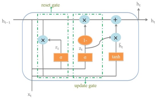
Figure 1. Basic GRU logical structure diagram.

The reset gate in GRU determines how to combine the new input information with the previous memory through the activation function $\sigma$, which is calculated as

$$r_t=\sigma (W_r·[h_{t-1},x_t])$$

(1)

where $W_r$ indicates the weight from the input layer to the hidden layer of the reset gate, $h_{t-1}$ is the hidden layer at time $t-1$, and $x_t$ indicates the input data at time t.

Candidate hidden layer status ${\tilde{h}}_t$ contains the input information of time t and selective retention of hidden layer state $h_{t-1}$. The calculation formula is

$${\tilde{h}}_t=tanh(W_h·[r_t·h_{t-1},x_t])$$

(2)

where $W_h$ is the weight of the hidden state.

The update gate defines the amount of previous memory saved to the current time step. The update gate calculation formula is

$$z_t=\sigma (W_z·[h_{t-1},x_t])$$

(3)

where $W_z$ indicates the weight from the input layer to the hidden layer of the update gate.

Finally, the hidden state decides how to combine a past hidden status and the current candidate information. The calculation formula is

$$h_t=(1-z_t)\ast h_{t-1}+z_t\ast {\tilde{h}}_t$$

(4)

The standard GRU network only considers the forward influence of historical information on future time series, overlooking the potential implicit information that may exist during network communication. To address this limitation, the BiGRU [35] model is introduced as a modification to the conventional GRU. By processing sequences of observations from both forward and reverse directions, as illustrated in Figure 2, the BiGRU network gains additional insights into the sequence. The primary objective of this approach is to extract maximal information from a given subsequence of observations, thereby providing an enhanced reference value for RUL prediction. Consequently, this paper adopts the BiGRU model in order to achieve this goal.

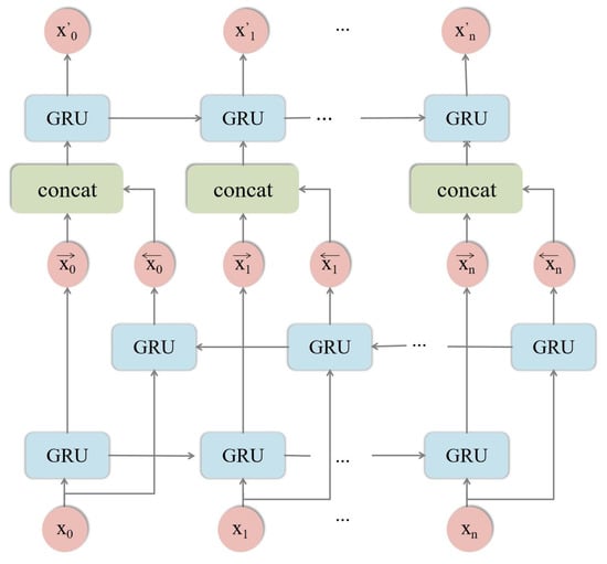
Figure 2. Structure diagram of building BiGRU.

2.2. Bayesian Neural Network and Improved Variational Inference

The Bayesian neural network is a powerful uncertainty framework [36]. It introduces uncertainty into a neural network by changing the constant weights (W in Figure 3) in the traditional neural network into probabilistic weights that obey a certain distribution; the structural comparison diagram is shown in Figure 3.

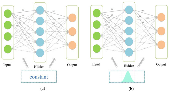
Figure 3. Structure comparison diagram of traditional neural network and Bayesian neural network. (a) traditional neural network; (b) bayesian neural network.

The basic idea of the Bayesian framework is to obtain model update knowledge, called posterior probability, from learned knowledge, called prior probability, and observed knowledge, called likelihood. Then, the model will be used to predict unknown samples. For a given training set $\{X,Y\}$, X represents the variable, and Y represents labels. Let $P\left(Y\right|X,w)$ be a model likelihood function, and let $P\left(w\right)$ be a model’s prior distribution. The posterior distribution is given by

$$P\left(w\right|X,Y)=\frac{P\left(Y\right|X,w\left)P\right(w)}{P\left(Y\right|X)}$$

(5)

For a new input data x, the Bayesian framework can output a probability distribution of the prediction variable y based on the new input data x and the historical data set $\{X,Y\}$. The predictive distribution is given as follows

$$P(y|x,X,Y)=\int P(y|x,w)P(w|X,Y)dw$$

(6)

Although the integral in Equation (6) is easy to calculate in the low-dimensional case, it is difficult to obtain the accurate posterior distribution $P\left(w\right|X,Y)$ in a deep neural network that contains high-dimensional parameters to obtain accurate integral value. To address this problem, approximation techniques are necessary. Currently, the two most popular approximation methods are the Markov chain Monte Carlo (MCMC) [37] and variational inference (VI) [38]. The MCMC, a sampling-based approach, does not require specific model assumption, but it is computationally expensive to obtain prediction results due to the need for obtaining a large number of samples of the posterior distribution. As a result, it is less suitable for problems with high-dimensional parameters. On the other hand, VI, an approximation-based method, requires the assumption of a prior model of the posterior distribution. However, it offers faster computation for generating prediction results. Considering the computational efficiency of the model, we employ VI in this study. Hypothetical prior distribution selection and distribution difference measurement are two key components in VI, which are introduced in detail as follows.

• Improved hypothetical prior distribution

Initially, a prior distribution of moderate complexity is carefully chosen. An overly simplistic model, while easier to optimize, may yield considerable approximation errors when attempting to approximate relatively complex distributions, thus compromising the accuracy of the approximate solution. Conversely, an excessively complex model, although capable of approximating any distribution, may introduce significant challenges in the optimization process. Previous studies have frequently employed Gaussian distributions for VI, but single Gaussian models often exhibit limited accuracy when approximating complex distributions.

In this research, we adopt a Gaussian mixture distribution as the prior distribution. The Gaussian mixture distribution comprises two individual Gaussian models with a mean value of ${\mu }_1,{\mu }_2$ and a variance value of ${\sigma }_1,{\sigma }_2$, providing a trade−off between computational complexity and prediction accuracy. The distribution is mathematically represented as follows:

$$Q\left(w\right|\theta )=\rho N\left(w\right|{\mu }_1,{\sigma }_1^2)+(1-\rho )N\left(w\right|{\mu }_2,{\sigma }_2^2)$$

(7)

where $\rho$ denotes the proportion of the mixture, and $\theta =\{{\mu }_1,{\mu }_2,{\sigma }_1,{\sigma }_2\}$ denotes the parameter set of the Gaussian mixture distribution.

• Distribution difference measurement

The Kullback–Leibler ($KL$) [39] divergence is a method to describe the difference between two probability distributions, P and Q. In neural networks, if P is unknown and we want to approximate it with a known distribution Q, the $KL$ divergence is usually taken as the error function, and the optimal approximate distribution Q can be obtained by minimizing the $KL$ divergence, which is calculated as

$$KL(Q\left(w\right|\theta )\parallel P\left(w\right|X,Y))=\int Q\left(w\right|\theta )log(\frac{Q\left(w\right|\theta )}{P\left(w\right|X,Y)})d\theta$$

(8)

In this work, a known probability distribution $Q\left(w\right|\theta )$ is directly used to approximate the posterior distribution $P\left(w\right|X,Y)$. We turn the posterior solution problem in Equation (6) into a parameter optimization problem by minimizing the $KL$ distance between $Q\left(w\right|\theta )$ and $P\left(w\right|X,Y)$. The formula is as follows

$${\theta }^{\ast }=argminKL(Q\left(w\right|\theta )\parallel P\left(w\right|X,Y))$$

(9)

According to the definition of $KL$ divergence in Equation (8), we rewrite the formula into the form of an expectation to facilitate the calculation results as

$$\begin{array}{ccc}\hfill KL\left(Q\right(w\left|\theta \right)\parallel P\left(w\right|X,Y\left)\right)& \propto & \hfill \\ \hfill E_{Q\left(w\right|\theta )}log\left[Q\left(w\right|\theta )\right]& -& E_{Q\left(w\right|\theta )}log\left[P\left(w\right)\right]-E_{Q\left(w\right|\theta )}log\left[P\left(Y\right|X,w)\right]\hfill \end{array}$$

(10)

Then, the loss function of our network consists of two parts: one is the loss of the network between the real RUL value and the predicted RUL value, which is measured by $MSE$, and the other one is the loss of uncertainty estimation, which is measured by $KL$. The final model loss function is defined as

$$Loss=MSELoss(y_{true},y_{pred})+KL(Q\left(w\right|\theta )\parallel P\left(w\right|X,Y))$$

(11)

where the $MSELoss$ is a loss function under the Pytorch frame, $y_{true}$ is the RUL label of the data set, and $y_{pred}$ is the RUL predicted by the model.

2.3. The RUL Probability Prediction Framework

This section will introduce the proposed probabilistic RUL prediction framework in this paper. The overall framework is depicted in Figure 4.

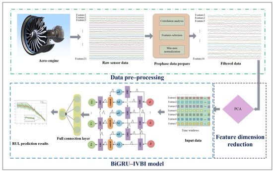
Figure 4. The overall RUL probability prediction framework.

First of all, the sensor data is subjected to a filtering process, where only pertinent information is retained and subsequently normalized using the minimum–maximum normalization technique, as in Equation (12). This normalization aims to mitigate the adverse effects arising from singular sample data.

$$x^{\ast }=\frac{x-x_{min}}{x_{max}-x_{min}}$$

(12)

where x is the sensor data, $x^{\ast }$ is normalized data, $x_{min}$ is the minimum value in the data, and $x_{max}$ is the maximum value in the data.

Then, the widely employed data compression technique, PCA, is applied. Numerous studies have demonstrated its significant impact on data dimensionality reduction and denoising. PCA is utilized to extract the principal features of the data, thereby reducing its dimensionality and enhancing the computational efficiency.

Subsequently, the core prediction model BiGRU-IVBI is composed by leveraging the Bayesian network into BiGRU. The deterministic weight value in BiGRU is replaced by our prior probability distribution to analyze the uncertainty factors in the neural network and train the model with gradient descent to minimize the loss function to obtain the optimal distribution parameters and, finally, obtain the RUL probability distribution prediction based on which the point prediction and CI of the aero-engine RUL prediction also can be obtained.

3. Experimental Study

3.1. Data Description

As shown in Figure 5, an aero-engine normally includes a fan, low-pressure compressor (LPC), low-pressure turbine (LPT), high-pressure compressor (HPC), high-pressure turbine (HPT) [2], and other modules. In this paper, the CMAPSS data set, which was generated by NASA using commercial modular aero-propulsion system simulation software for PHM themed competitions, is used for experiments. The data comes from turbofan engines, and each engine has 21 sensors. There are four data sets under different conditions; we choose FD001 as the experimental data set which was conducted under a single fault, i.e., the degradation of the high-pressure compressor, including the training set and test set. The number of training samples is 17,631, and the model is tested on 100 engines with a total of 10,096 samples. Specific information about the sensors is displayed in Table 1.

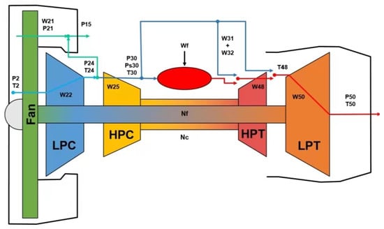
Figure 5. Schematic representation of the aero-engine model [40].

Table 1. Description of sensor data.

Index	Symbol	Description	Units
1	T2	Total temperature at fan inlet	${}^o$R
2	T24	Total temperature at LPC outlet	${}^o$R
3	T30	Total temperature at HPC outlet	${}^o$R
4	T50	Total temperature at LPT outlet	${}^o$R
5	P2	Pressure at fan inlet	psia
6	P15	Total pressure in bypass-duct	psia
7	P30	Total pressure at HPC outlet	psia
8	Nf	Physical fan speed	rpm
9	Nc	Physical core speed	rpm
10	epr	Engine pressure ratio (P50/P2)	-
11	Ps30	Static pressure at HPC outlet	psia
12	phi	Ratio of fuel flow to Ps30	pps/psi
13	NRf	Corrected fan speed	rpm
14	NRc	Corrected core speed	rpm
15	BPR	Bypass ratio	-
16	farB	Burner fuel–air ratio	-
17	htBleed	Bleed enthalpy	-
18	Nf_dmd	Demanded fan speed	rpm
19	PCNfR_dmd	Demanded corrected fan speed	rpm
20	W31	HPT coolant bleed	lbm/s
21	W32	LPT coolant bleed	lbm/s

3.2. Data Pre-Processing

• Data visualization and analysis

We first visualize the original monitoring data in Figure 6 to better observe the data characteristics. It can be observed from the above picture that not all of the sensor data contain useful information; some sensor data remain unchanged. It is noteworthy that although sensor 6 has fluctuation, it is just some noise.

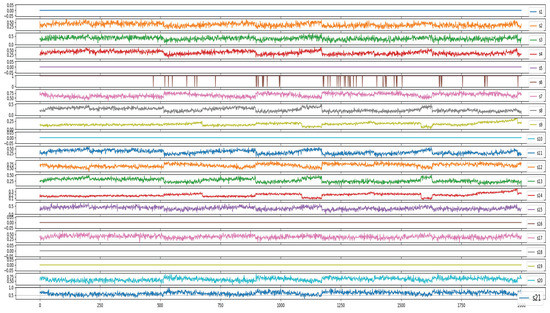
Figure 6. 21 characteristic data of sensors.

• Correlation analysis

We also conduct correlation analysis between the sensor data and RUL. As can be seen from Figure 7, some sensor data have no correlation information, so we combine the results of the data visualization in Figure 6 and finally decide to reject the data from sensors 1, 5, 6, 10, 16, 18, and 19. We also found that some sensor data show a high correlation, indicating the existence of some redundancy features. It is necessary to extract the main features.

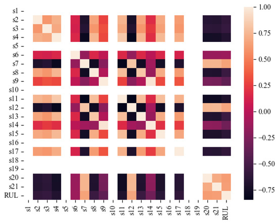
Figure 7. Correlation between sensor data and RUL.

3.3. Principal Component Analysis

Next, the data features are extracted by PCA. As shown in Figure 8, the first seven principal components can contain more than $90\%$ of the information of the raw data. So the first seven principal component features are selected.

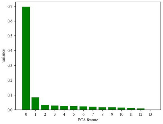
Figure 8. Information proportion of variance of principal components.

3.4. Evaluation Metrics

The performance is evaluated from four indicators, including the root mean squared error ($RMSE$), mean absolute error ($MAE$), symmetric mean absolute percentage error ($SMAPE$), and score function ($Score$). These indicators are defined as follows

$$RMSE=\sqrt{\frac{1}{n}\sum _{i=1}^n{(y_{pre{d}_i}-y_{tru{e}_i})}^2}$$

(13)

$$MAE=\frac{1}{n}\sum _{i=1}^n|y_{pre{d}_i}-y_{tru{e}_i}|$$

(14)

$$SMAPE=\frac{100\%}{n}\sum _{i=1}^n\frac{|y_{pre{d}_i}-y_{tru{e}_i}|}{\left(\right|y_{pre{d}_i}|+|y_{tru{e}_i}\left|\right)/2}$$

(15)

$$Score=\left\{\begin{array}{c}{\displaystyle \sum _{i=1}^n}{e}^{-\frac{y_{pre{d}_i}-y_{tru{e}_i}}{13}}-1, y_{pre{d}_i}-y_{tru{e}_i}<0\hfill \\ {\displaystyle \sum _{i=1}^n}{e}^{\frac{y_{pre{d}_i}-y_{tru{e}_i}}{10}}-1, y_{pre{d}_i}-y_{tru{e}_i}\ge 0.\hfill \end{array}\right.$$

(16)

where n is the number of test samples, $y_{pred}$ denotes the predicted RUL, and $y_{true}$ denotes the real RUL. RMSE is selected to measure the deviation between the prediction RUL and the real RUL. MAE is more robust to outliers. SMAPE can represent the quality of the model. Score is a scoring used in the 2008 PHM management data challenge.

3.5. Experimental Results

There are 100 engines in the data set. Here, we choose engine No. 21, No. 35, No. 51, and No. 100 as examples. The RUL prediction results are shown in Figure 9.

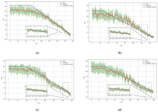
Figure 9. RUL prediction results of four engines: (a) engine No. 21; (b) engine No. 35; (c) engine No. 51; (d) engine No. 100.

The figures show that there is great uncertainty in the initial stage. Then, the CI gradually narrows as the aero-engine degrades, and, finally, the fault interval is accurately predicted. From the partially enlarged image, it can be seen that even if the point prediction does not completely overlap with the real-life degradation curve, the CI can still provide a reliable prediction range. The same conclusion can be made from the results of other engines in the data set, which are not displayed due to the space limitation.

To illustrate the effectiveness of the BiGRU-IVBI model in the proposed method more comprehensively, under the same network configuration conditions, we compared our model with the Bayesian multi-layer perception (BMLP), Bayesian long short-term memory (BLSTM), Bayesian gate recurrent unit (BGRU), and Bayesian bidirectional long short-term memory (BBiLSTM) models. Table 2 shows the RUL prediction results of the comparison with $95\%$ CI. It can be clearly seen from the data in Table 2 that our BiGRU-IVBI method has the best performance among the four models with the lowest RMSE, MAE, Score, and SMAPE. To make the results more intuitive, a line chart is also provided in Figure 10.

Table 2. Prediction performance comparison with other models.

	RMSE	MAE	Score	SMAPE (%)
BMLP	37.90	35.09	22.34	38.80
BLSTM	25.13	20.08	9.05	23.16
BGRU	24.58	19.49	8.33	22.07
BBiLSTM	11.04	10.30	3.02	13.23
BiGRU-IVBI	9.91	7.60	1.84	11.96
BiGRU-IVBI (non-PCA)	11.47	9.43	2.75	13.86

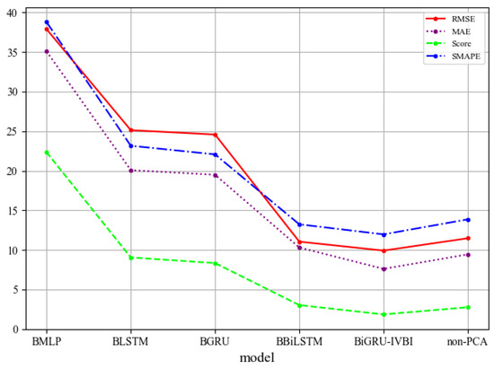
Figure 10. Evaluation indexes based on different models.

Simultaneously, we conducted an experiment using unprocessed data without the PCA feather-extraction process. It is evident from Table 2 and Figure 10 that the experimental results are inferior to the results obtained using PCA, which explains the effectiveness of PCA in improving the prediction results. All of the above results indicate that our model is feasible and is the most cost-effective one.

As seen in Table 3, we compare the proposed method with some advanced methods on the CMAPSS data sets mentioned in the literature, and the results show that our method has a significant improvement in the RMSE on data set FD001. This means that the RUL predicted by our proposed method is closer to the real RUL and achieves more satisfactory accuracy.

Table 3. The comparison of different methods with CMAPSS data sets.

Methods and References	RMSE
MODBNE [19]	17.96
DCNN [20]	12.61
LightGBM [21]	12.79
MT-CNN [22]	12.48
MLSA [24]	11.57
BiLSTM [25]	11.96
IDMFFN [26]	12.18
LSTM [27]	11.80
BiGRU-IVBI	9.91

We also conducted comparative experiments for different window sizes and finally set the window size to $T=30$. The comparative experimental results of the different window sizes are shown in Table 4 and Figure 11.

Table 4. RUL prediction comparison with different time window size.

Window Size	RMSE	MAE	Score	SMAPE (%)
20	16.00	12.46	4.39	22.02
30	9.91	7.60	1.84	11.96
40	10.16	8.47	1.96	14.37
50	14.06	10.05	2.19	15.97

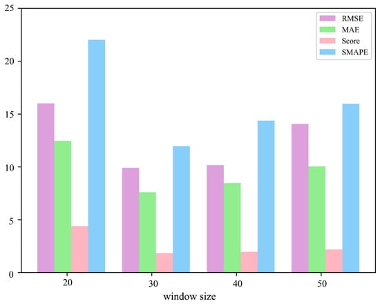
Figure 11. Comparative experimental results of different window size.

In order to illustrate the effect of the parameter $\rho$ in the Gaussian mixture model on the prediction performance, we also compare the experimental results of several Gaussian mixture models with different mixing ratios $\rho$, and the comparison results are shown in Table 5 and Figure 12. In order to ensure the fairness of the experiment, the average value of five experiments is taken for all of the above test data.

Table 5. Experimental comparison results of different $\rho$:

Model	RMSE	MAE	Score	SMAPE (%)
$\rho$ = 0	13.85	11.67	4.16	16.25
$\rho$ = 0.25	9.91	7.60	1.84	11.96
$\rho$ = 0.50	11.85	9.44	2.67	12.76
$\rho$ = 0.75	13.88	11.19	4.05	15.34
$\rho$ = 1.00	14.43	11.27	4.34	16.87

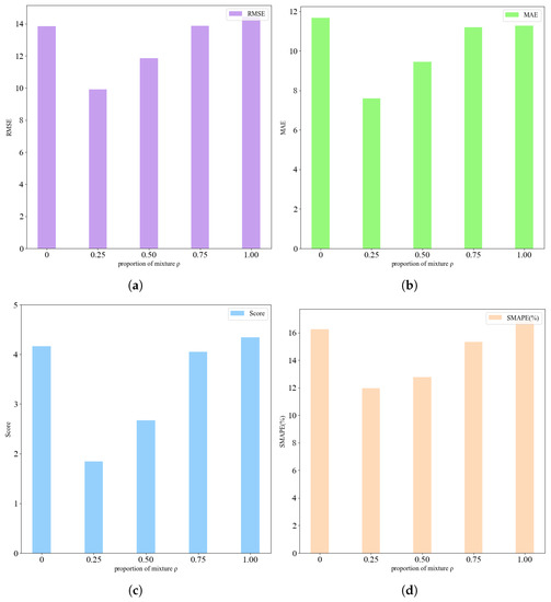
Figure 12. Comparison results of different $\rho$.

We regularly take $\rho$ within the range from 0 to 1 with a step size of 0.25. It can be found from the table and the figure that the RUL prediction error of the network is at its minimum when $\rho =0.25$. It is worth noting that the prior of the Gaussian mixture distribution used in this paper will degenerate to a single Gaussian distribution when $\rho =0$ and $\rho =1$. The experimental results show that the prior of the Gaussian mixture distribution used in this paper has certain advantages in probability RUL prediction and can be extended to other RUL predictions.

4. Conclusions

A novel aero-engine RUL probability prediction framework based on BiGRU-IVBI is proposed in this paper, which takes into account the uncertainties during the degradation process of aero-engines. The representative features are first extracted by the PCA algorithm. Then, the BiGRU network is trained for RUL prediction with prediction uncertainties quantified by the proposed IVBI method, where the Gaussian mixture distribution is introduced to improve the generalization capability and prediction accuracy of the traditional variational Bayesian inference approach. The proposed method can give not only the point estimate of RUL prediction but also the CI of the estimate, which is of great importance for real-world application. Finally, the performance of the proposed method is verified on the CMAPSS data set, and the prediction accuracy is higher than other comparative models, which proves the effectiveness and superiority of the proposed framework.

Further research will be committed to finding more effective uncertainty prediction methods to obtain a higher RUL prediction accuracy. At the same time, exploring the application of the proposed method to the RUL prediction in situations where multiple degradation mechanisms are in place is also the direction of our future research.

References

- Che, C.; Wang, H.; Fu, Q.; Ni, X. Combining multiple deep learning algorithms for prognostic and health management of aircraft. Aerosp. Sci. Technol. 2019, 94, 105423. [Google Scholar] [CrossRef]
- Huang, Y.; Sun, G.; Tao, J.; Hu, Y.; Yuan, L. A modified fusion model-based/data-driven model for sensor fault diagnosis and performance degradation estimation of aero-engine. Meas. Sci. Technol. 2022, 33, 085105. [Google Scholar] [CrossRef]
- Volponi, A.J. Gas turbine engine health management: Past, present, and future trends. J. Eng. Gas Turbines Power 2014, 136, 051201-1. [Google Scholar] [CrossRef]
- Li, T.; Si, X.; Pei, H.; Sun, L. Data-model interactive prognosis for multi-sensor monitored stochastic degrading devices. Mech. Syst. Signal Process. 2022, 167, 108526. [Google Scholar] [CrossRef]
- Soualhi, A.; Lamraoui, M.; Elyousfi, B.; Razik, H. PHM survey: Implementation of prognostic methods for monitoring industrial systems. Energies 2022, 15, 6909. [Google Scholar] [CrossRef]
- Sadeghkouhestani, H.; Yi, X.; Qi, G.; Liu, X.; Wang, R.; Gao, Y.; Yu, X.; Liu, L. Prognosis and health management (PHM) of solid-state batteries: Perspectives, challenges, and opportunities. Energies 2022, 15, 6599. [Google Scholar] [CrossRef]
- Kong, Z.; Cui, Y.; Xia, Z.; Lv, H. Convolution and Long Short-Term Memory Hybrid Deep Neural Networks for Remaining Useful Life Prognostics. Appl. Sci. 2019, 9, 4156. [Google Scholar] [CrossRef]
- Huang, B.; Cohen, K.; Zhao, Q. Active anomaly detection in heterogeneous processes. IEEE Trans. Inf. Theory 2019, 65, 2284–2301. [Google Scholar] [CrossRef]
- Nguyen, V.; Seshadrinath, J.; Wang, D.; Nadarajan, S.; Vaiyapuri, V. Model-based diagnosis and RUL estimation of induction machines under interturn fault. IEEE Trans. Ind. Appl. 2017, 53, 2690–2701. [Google Scholar] [CrossRef]
- Wei, H.; Zhang, Q.; Gu, Y. Remaining useful life prediction of bearings based on self-attention mechanism, multi-scale dilated causal convolution, and temporal convolution network. Meas. Sci. Technol. 2023, 34, 045107. [Google Scholar] [CrossRef]
- Barraza-Barraza, D.; Tercero-Gomez, V.G.; Beruvides, M.G.; Limón-Robles, J. An adaptive ARX model to estimate the RUL of aluminum plates based on its crack growth. Mech. Syst. Signal Process. 2017, 82, 519–536. [Google Scholar] [CrossRef]
- Liu, Y.; Zuo, M.J.; Li, Y.F.; Huang, H.Z. Dynamic reliability assessment for multi-state systems utilizing system-level inspection data. IEEE Trans. Reliab. 2015, 64, 1278–1299. [Google Scholar] [CrossRef]
- Wang, C.; Lu, N.; Cheng, Y.; Jiang, B. A data-driven aero-engine degradation prognostic strategy. IEEE Trans. Cybern. 2021, 51, 1531–1541. [Google Scholar] [CrossRef] [PubMed]
- Zhao, H.; Liu, H.; Jin, Y.; Dang, X.; Deng, W. Feature extraction for data-driven remaining useful life prediction of rolling bearings. IEEE Trans. Instrum. Meas. 2021, 70, 1–10. [Google Scholar] [CrossRef]
- Qian, Y.; Yan, R.; Hu, S. Bearing degradation evaluation using recurrence quantification analysis and kalman filter. IEEE Trans. Instrum. Meas. 2014, 63, 2599–2610. [Google Scholar] [CrossRef]
- Wang, Z.; Wen, C.; Dong, Y. A method for rolling bearing fault diagnosis based on GSC-MDRNN with multi-dimensional input. Meas. Sci. Technol. 2023, 34, 055901. [Google Scholar] [CrossRef]
- Ren, L.; Zhao, L.; Hong, S.; Zhao, S.; Wang, H.; Zhang, L. Remaining useful life prediction for lithium-ion battery: A deep learning approach. IEEE Access 2018, 6, 50587–50598. [Google Scholar] [CrossRef]
- Wang, W.; Zhang, L.; Yu, H.; Yang, X.; Zhang, T.; Chen, S.; Liang, F.; Wang, H.; Lu, X.; Yang, S. et al. Early prediction of the health conditions for battery cathodes assisted by the fusion of feature signal analysis and deep-learning techniques. Batteries 2022, 8, 151. [Google Scholar] [CrossRef]
- Zhang, C.; Lim, P.; Qin, A.K.; Tan, K.C. Multiobjective deep belief networks ensemble for remaining useful life estimation in prognostics. IEEE Trans. Neural Netw. Learn. Syst. 2017, 28, 2306–2318. [Google Scholar] [CrossRef]
- Li, X.; Ding, Q.; Sun, J.Q. Remaining useful life estimation in prognostics using deep convolution neural networks. Reliab. Eng. Syst. Saf. 2018, 172, 1–11. [Google Scholar] [CrossRef]
- Liu, L.; Wang, L.; Yu, Z. Remaining useful life estimation of aircraft engines based on deep convolution neural network and LightGBM combination model. Int. J. Comput. Intell. Syst. 2021, 14, 165. [Google Scholar] [CrossRef]
- Kim, T.S.; Sohn, S. Multitask learning for health condition identification and remaining useful life prediction: Deep convolutional neural network approach. J. Intell. Manuf. 2021, 32, 2169–2179. [Google Scholar] [CrossRef]
- Liu, J.; Lei, F.; Pan, C.; Hu, D.; Zuo, H. Prediction of remaining useful life of multi-stage aero-engine based on clustering and LSTM fusion. Reliab. Eng. Syst. Saf. 2021, 214, 107807. [Google Scholar] [CrossRef]
- Xia, J.; Feng, Y.; Lu, C.; Fei, C.; Xue, X. LSTM-based multi-layer self-attention method for remaining useful life estimation of mechanical systems. Eng. Fail. Anal. 2021, 125, 105385. [Google Scholar] [CrossRef]
- Jin, R.; Chen, Z.; Wu, K.; Wu, M.; Li, X.; Yan, R. Bi-LSTM-based two-stream network for machine remaining useful life prediction. IEEE Trans. Instrum. Meas. 2022, 71, 1–10. [Google Scholar] [CrossRef]
- Li, X.; Jiang, H.; Liu, Y.; Wang, T.; Li, Z. An integrated deep multiscale feature fusion network for aeroengine remaining useful life prediction with multisensor data. Knowl.-Based Syst. 2022, 235, 107652. [Google Scholar] [CrossRef]
- Song, T.; Liu, C.; Wu, R.; Jin, Y.; Jiang, D. A hierarchical scheme for remaining useful life prediction with long short-term memory networks. Neurocomputing 2022, 487, 22–33. [Google Scholar] [CrossRef]
- Caceres, J.; Gonzalez, D.; Zhou, T.; Droguett, E.L. A probabilistic Bayesian recurrent neural network for remaining useful life prognostics considering epistemic and aleatory uncertainties. Struct. Control. Health Monit. 2022, 28, 1545–2255. [Google Scholar] [CrossRef]
- Kraus, M.; Feuerriegel, S. Forecasting remaining useful life: Interpretable deep learning approach via variational Bayesian inferences. Decis. Support Syst. 2019, 125, 113100. [Google Scholar] [CrossRef]
- Zu, T.; Kang, R.; Wen, M. Graduation formula: A new method to construct belief reliability distribution under epistemic uncertainty. J. Syst. Eng. Electron. 2020, 31, 626–633. [Google Scholar]
- Li, G.; Yang, L.; Lee, C.G.; Wang, X.; Rong, M. A Bayesian deep learning RUL framework integrating epistemic and aleatoric uncertainties. IEEE Trans. Ind. Electron. 2021, 68, 8829–8841. [Google Scholar] [CrossRef]
- Wang, C.; Miao, X.; Zhang, Q.; Bo, C.; Zhang, D.; He, W. Similarity-based probabilistic remaining useful life estimation for an aeroengine under variable operational conditions. Meas. Sci. Technol. 2022, 33, 114011. [Google Scholar] [CrossRef]
- Jiao, R.; Peng, K.; Dong, J. Remaining useful life prediction for a roller in a hot strip mill based on deep recurrent neural networks. IEEE/CAA J. Autom. Sin. 2021, 8, 1345–1354. [Google Scholar] [CrossRef]
- Long, B.; Wu, K.; Li, P.; Li, M. A novel remaining useful life prediction method for hydrogen fuel cells based on the gated recurrent unit neural network. Appl. Sci. 2021, 12, 432. [Google Scholar] [CrossRef]
- She, D.; Jia, M. A BiGRU method for remaining useful life prediction of machinery. Measurement 2021, 167, 108277. [Google Scholar] [CrossRef]
- Zaidan, M.A.; Mills, A.R.; Harrison, R.F.; Fleming, P.J. Gas turbine engine prognostics using Bayesian hierarchical models: A variational approach. Mech. Syst. Signal Process. 2016, 71, 120–140. [Google Scholar] [CrossRef]
- Pei, H.; Si, X.; Hu, C.; Li, T.; He, C.; Pang, Z. Bayesian deep-learning-based prognostic model for equipment without label data related to lifetime. IEEE Trans. Syst. Man Cybern. Syst. 2023, 53, 504–517. [Google Scholar] [CrossRef]
- Gao, Z.; Tao, J.; Su, Y.; Zhou, D.; Zeng, X.; Li, X. Efficient rare failure analysis over multiple corners via correlated Bayesian inference. IEEE Trans. Comput.-Aided Des. Integr. Circuits Syst. 2020, 39, 2029–2041. [Google Scholar] [CrossRef]
- Ping, G.; Chen, J.; Pan, T.; Pan, J. Degradation feature extraction using multi-source monitoring data via logarithmic normal distribution based variational auto-encoder. Comput. Ind. 2019, 109, 72–82. [Google Scholar] [CrossRef]
- Arias Chao, M.; Kulkarni, C.; Goebel, K.; Fink, O. Aircraft Engine Run-to-Failure Dataset Under Real Flight Conditions for Prognostics and Diagnostics. Data 2021, 6, 5. [Google Scholar] [CrossRef]
Disclaimer/Publisher’s Note: The statements, opinions and data contained in all publications are solely those of the individual author(s) and contributor(s) and not of MDPI and/or the editor(s). MDPI and/or the editor(s) disclaim responsibility for any injury to people or property resulting from any ideas, methods, instructions or products referred to in the content. |
© 2023 by the authors. Licensee MDPI, Basel, Switzerland. This article is an open access article distributed under the terms and conditions of the Creative Commons Attribution (CC BY) license (https://creativecommons.org/licenses/by/4.0/).