MDPN: Multilevel Distribution Propagation Network for Few-Shot Image Classification

Abstract

Due to a shortage of labeled examples, few-shot image classification frequently experiences noise interference and insufficient feature extraction. In this paper, we present a two-stage framework based on the distribution propagation graph neural network (DPGN) called the multilevel distribution propagation network (MDPN). An instance-segmentation-based object localization (ISOL) module and a graph-based multilevel distribution propagation (GMDP) module are both included in the MDPN. To create a clear and full object zone, the ISOL module generates a mask that eliminates background and pseudo-object noises. The GMDP module enriches the level of features. We carried out comprehensive experiments on the few-shot dataset CUB-200-2011 to show the usefulness of MDPN. The results demonstrate that MDPN indeed outperforms DPGN in terms of few-shot image classification accuracy. Under 5-way 1-shot and 5-way 5-shot settings, the classification accuracy of MDPN exceeds the baseline by 8.17% and 1.24%, respectively. MDPN also outperforms the majority of the existing few-shot classification methods in the same setting.

1. Introduction

A significant amount of labeled data is needed for traditional deep-learning techniques. However, there are times when there are very few samples accessible because of the security, morality, resource, and expense concerns associated with data collection. Few-shot learning (FSL) was used to find a solution to this issue. FSL seeks to develop models that perform well when trained on small-scale data. Additionally, FSL can significantly lower the cost of manual annotation and has a broad range of potential applications in data-scarce areas such as uncommon disease data and human-computer interaction.

However, the backbone can only be set up as a lightweight network with shallow depth and narrow width, such as ConvNet4, Resnet12 [1], Resnet18, WRN-28-10, etc., to minimize underfitting because of the limited quantity of labeled data in FSL. Lightweight backbones can typically only do straightforward feature extraction; therefore, additional post-processing is required. We discovered that several studies have demonstrated that deep networks [2,3] integrate shallow, intermediate, and high levels of image features [4]. As network layers are added, the “level” of features steadily gets richer. Higher layers of the network pay more attention to the semantic information in the image, whereas lower layers concentrate more on the detailed information. This is true because the receptive fields in lower layers are typically smaller and their overlapping regions are smaller than those in higher levels. As a result, the lower layers of the network can acquire more precise information. The receptive fields and the overlap regions gradually expand with increasing downsampling. The expression of one pixel in the feature map corresponds to a certain region’s information in the original image, which contains more in-depth abstract information, or semantic information. In this paper, we present a multilevel feature extraction module to get different levels of features by stacking graph neural networks (GNNs) in sequence, with the goal of improving the feature extraction capability of the lightweight backbone.

The impact of noise on prediction accuracy will be particularly clear when the backbone of FSL has limited feature extraction capabilities. The dataset CUB 200-2011 that we utilize in particular for our research is a dataset of birds in a natural scene. The backgrounds of the birds in CUB 200-2011 primarily consist of the sky, branches, flowers, stones, and water, as seen in Figure 1. These backgrounds are intricate, and occasionally the birds even blend in with them. Eliminating pseudo-object interference and precisely extracting the target object from the image in FSL is also a big challenge for the model. As shown in Figure 2, several types of bird images contain a particular sort of pseudo-object, such as human hands, tree stumps, cages, water dispensers, oranges, etc. When a specific type of pseudo-object is included in the support set and query set of an episode (support set, query set, and episode are all words used in the FSL domain). An episode means a task; the support set equals the training set, and the query set equals the testing set. The model may mistakenly treat the pseudo-object as the target object and misclassify the two photos of distinct types of birds as belonging to the same category. In this study, we present an instance-segmentation-based object localization module that creates a new picture containing only the target object by precisely segmenting along the object’s edge in order to exactly remove the interference of backdrop and pseudo-object.

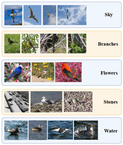
Figure 1. Complex backgrounds in CUB-200-2011.

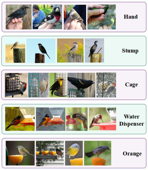
Figure 2. Variable pseudo-objects in CUB-200-2011.

In this paper, we present an MPDN for few-shot image classification that combines an instance-segmentation-based object localization (ISOL) module with a graph-based multilevel distribution propagation (GMDP) module to address these issues. The instance segmentation adopted by the ISOL module is based on prior knowledge. Using the previously known segmentation of the images, ISOL divides the raw images into segments based on the outer contour of the target object and masks the non-object portions. The final outputs of ISOL are the regions included in each object’s minimum bounding rectangle (MBR). The GMDP module, which consists of three graph networks concatenated in series, is used to post-process the features. The outcomes of GPDN are three layers of distributions with increasing abstraction. We then use these three distributions to update the original features that were supplied to the GMDP module, and we send the revised features back to the module to be used in the following iteration. Iterations serve the objective of making the final output features contain the information of the entire graph by repeatedly computing the distribution.

The steps for training the MDPN are as follows: Images are first supplied to the ISOL module. The ISOL module crops the images in accordance with the object’s MBR. After that, the cropped images are sent to the backbone to extract features. The GMDP module is then used to extract the three levels of distribution features from the object features, which are subsequently utilized to update the original object features. Following a number of iterations in the GMDP module, the cross-entropy loss between the output features of the GMDP module and the ground truth labels is determined.

Our main contributions are as follows:

• As far as we are aware, MDPN is the first model to stack graph networks in series to extract several levels of distribution in few-shot image classification. Our follow-up ablation trials have shown its usefulness.
• In order to increase the precision and completeness of the localization, we incorporated past knowledge into the target object region localization by utilizing segmentation information. The accuracy of the prior-knowledge-based method is significantly higher than that of the supervised-learning-based target area localization method.
• We perform in-depth analyses on the CUB-200-2011 dataset. In both 5-way 1-shot and 5-way 5-shot settings, the classification accuracy of MDPN outperforms the baseline by 8.17% and 1.24%, respectively. In the same setting, it outperforms most of the existing few-shot classification methods.

2. Related Work

2.1. Few-Shot Learning

Few-shot learning (FSL) can be broadly categorized into three ways: (1) using external memory; (2) introducing previous knowledge into the model initialization parameters; and (3) using training data as prior knowledge.

The first way to use external memory is to store training characteristics in an external memory and then compare test features with the features read from the external memory to predict the label of the test sample. Santoro et al. [5] first put forward the idea of using external memory to perform FSL problems in 2016, and their proposed memory-augmented neural network (MANN) can overcome the concerns with LSTM [6] instability. MetaNet [7], proposed by Munkhdalai et al., combines external memory and meta-learning. Qi Cai et al. [8] proposed a memory matching network that uses storage support features and the corresponding category labels to form “key-value pairs” in a memory module. Kaiser et al. [9] proposed a lifelong memory module that uses the k-nearest neighbor (KNN) to select k samples that are closest to the query sample and predicts the label of the sample. However, it should be noted that the extra storage space will increase the cost of training.

The second strategy, known as meta-learning, enables the model to learn how to learn by embedding prior knowledge into the model initialization parameters. MAML [10], a gradient-based method proposed by Finn et al. in 2017, designs a me-ta-learner as an optimizer to update model parameters with only a few optimization steps when given novel examples. The MAML-based Meta-SGD [11] algorithm can learn both the direction and the pace of optimization. Additionally, Nichol et al. [12] proposed Reptile in 2018, which greatly reduces the computational complexity by avoiding the computation of two derivatives in MAML. MetaOptNet [13] proposed replacing the nearest-neighbor method with a linear classifier that can be optimized for convex optimization learning.

The ways of using training data as prior knowledge are further divided into finetuning-based methods and metric-based methods. The goal of the former is to train the model using a lot of auxiliary data and then fine-tune it using the target few-shot dataset. The latter’s goal is to create a network that can distinguish between several classes by doing feature distance analysis. Many classical networks for few-shot classification are based on metric-based methods. MatchingNet [14] generates a weighted nearest neighbor classifier by computing the mapping distance between the support set and the query set. ProtoNet [15], proposed by Snell et al., extracts prototype features from samples of the same category and then predicts them by comparing the Euclidean distance between query features and prototype features. RelationNet [16] uses an adaptive nonlinear classifier to measure the relationship between support features and query features.

2.2. Attention Mechanism

The attention technique was initially employed in the machine translation problem and is now extensively used in several deep learning disciplines [4,17]. Humans selectively focus on a portion of all information while disregarding others due to the information processing bottleneck. Similar to how a human brain analyzes information, a neural network employs its attention mechanism to quickly focus on a small subset of important data.

Class activation mapping (CAM) [18] has recently gotten more and more attention. CAM works as follows: first, delete the convolutional neural network’s (CNN) last fully connected layers; Secondly, substituting a global average pooling (GAP) layer for the maxpooling layer; computing the characteristics’ weighted average comes last. However, it must change CNN’s structure, and accuracy must be gradually increased by training, which slows the model’s convergence rate. Then, a variety of enhanced CAMs have been put out to expand CAM to more intricate CNN structures: Grad-CAM [19] relies on gradients to weight features learned in the final convolutional layer and generalizes CAM without changing the model. Grad-CAM++ [20] improves Grad-CAM visualization by weighting the gradients pixel by pixel. CBAM [21] is a lightweight general-purpose module that can be smoothly integrated into any convolutional neural network architecture [22] to participate in end-to-end training. It infers the attention map along two distinct dimensions (channel and spatial).

Since the attention mechanism needs to be optimized over several iterations, it is time-consuming and not easy to locate and cover the entire object. The accuracy of the activation mechanism generally remains low because it often only focuses on a part of the object and may capture a lot of pointless information. We use instance segmentation methods in our object localization module to achieve accurate localization in order to prevent information redundancy and misinformation. The instance segmentation method approach accurately and completely obtains objects by masking off non-object regions to eliminate the interference of background and pseudo-objects. It makes feature extraction more effective.

2.3. Graph Neural Network

GNN has been heavily utilized in FSL recently. Garcia et al. [23] first suggested using GNN to solve few-shot image classification in 2018. They proposed to treat each sample as a node in the graph and use GNN to learn and update the embedding of the node, and then update the edge vector through the node vector. To further capitalize on intra-class similarities and inter-class differences, the conduction propagation network (TPN) [24] proposed by Liu et al. leverages the complete query set for inference.

Kim et al. [25] proposed an edge-labeled graph neural network, where the two dimensions of edge features correspond to the intra-class similarity and the inter-class difference of the two nodes connecting the edge, and then binary classification is performed to determine whether two nodes belong to the same class. Yang et al. [26] proposed the distribution propagation graph neural network (DPGN), which constructs an explicit class distribution relationship. Gidaris et al. [27] added denoising autoencoders (DAE) to GNN to correct the weights of few-shot categories. The GNN-based model is significant and should be explored widely because of its powerful information propagation and relationship expression abilities. Zhang et al. [28] proposed a graph information aggregation cross-domain few-shot learning (Gia-CFSL) framework, intending to mitigate the impact of domain shift on FSL through domain alignment based on graph information aggregation. Zhong et al. [29] presented a graph-complemented latent representation (GCLR) network for few-shot image classification to learn a better representation. A GNN is added to relational mining to better utilize the relationship between samples in each category.

3. Proposed Method

We propose an MDPN framework that contains an ISOL module and a GMDP module. Different from the attention mechanism method mentioned in Section 2.2, which does not eliminate noise completely, the ISOL module completely eliminates background and pseudo-objects by generating masks so as to obtain a clean and complete target area. Different from the GNN methods mentioned in Section 2.3, which all use GNNS alone or stacked in parallel, the GMDP module obtains richer features with deeper abstraction levels layer by layer through series-stacked GNNs. As shown in Figure 3, MDPN first sends the input images to the ISOL module, which is based on instance segmentation. For each input image, the ISOL module creates a new image that only contains the object region. Then, the new images are sent to the backbone to obtain the object features. After that, three levels of distribution features of the object features are extracted by the GMDP module and then used to update the object features. The updated object features go on to the next iteration. We calculate the class prediction using the updated object features at the end of each iteration.

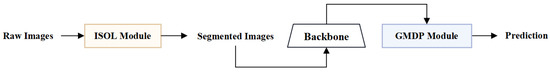
Figure 3. The abstract flow of multilevel distribution propagation network (MDPN).

3.1. Problem Definition

In standard few-shot classification, there are two datasets: the training set $D_{base}=\left\{\left(x_i,y_i\right),y_i\in C_{base}\right\}$ and the test set $D_{novel}=\left\{\left(x_i,y_i\right),y_i\in C_{novel}\right\}$, where $C_{base}$ and $C_{novel}$ represent the base classes in the training set and novel classes in the test set, and they do not overlap ($C_{base}\cap C_{novel}=\varnothing$). Training and testing for few-shot image classification consist of a number of episodes. Each episode is constructed by randomly sampling K categories, which consist of N labeled images and U unlabeled images, i.e., the k-way n-shot setting. The labeled images are called support set $S={\left\{\left(x_i,y_i\right)\right\}}_{j=1}^{K\times N}$, and the unlabeled images are called query set $Q={\left\{\left(x_i,y_i\right)\right\}}_{j=1}^{K\times U}$, where they do not overlap ($S\cap Q=\varnothing$).

Take the 5-way 1-shot (that is, K = 5, N = 1) episode setting as an instance:

(1)

Divide the dataset into a training set $D_{base}$ and a test set $D_{novel}$ by category.

(2)

Sample five categories from $D_{base}$. Then, sample 1 image from each category as a labeled image to form the support set S, and U images from each category as unlabeled images to form the query set Q (U can be set according to your needs, such as 1, 15, etc.). In our experiment, U = 1, $S\cap Q=\varnothing$.

The model learns the features of the images in S according to the specific algorithm and predicts the labels of the images in Q. Calculate the loss between predicted labels and ground truth labels, then backpropagate the loss.

(3)

Repeat step (2) until the preset number of episodes is reached.

(4)

Sample five categories from $D_{novel}$. Then, sample 1 image from each category as a labeled image to form support set $S\prime$ and $U\prime$ images from each category as unlabeled images to form query set Q′ ($U\prime$ can be set according to your needs, such as 1, 15, etc.). In our experiment, $U\prime$=1, $S\prime \cap \mathrm{Q}\prime =\varnothing$.

(5)

Repeat step (4) until the preset number of episodes is reached.

(6)

Repeat steps from (2) to (5) until the preset number of epochs is reached.

The K-way N-shot setting aims to train a classifier that can accurately map a query set to its label based only on a small support set. The 5-way setting is chosen in our experiments instead of more categories, such as 20-way, 36-way, 50-way, etc. [30,31,32] Compared to the Q-way (Q > 5), the 5-way setting requires less data to reduce the risk of model overfitting and is more suitable for training with a small amount of data or limited time. Therefore, we use a 5-way setting in our study.

3.2. Instance-Segmentation-Based Object Localization

CNN typically extracts features from the entire image, regardless of the background or target object. Images of natural scenes, however, contain complex backgrounds and some pseudo-objects. Consequently, CNN may extract irrelevant or even interfering features, which is particularly detrimental to subsequent class predictions. Therefore, before extracting features, it is crucial to locate the target object. Based on prior knowledge of segmentation images, we propose an object localization method in our ISOL module. Prior knowledge, as we all know, is knowledge that existed before an experience. When a person learns something new, their brain will naturally make references to previously learned information. The brain will quickly assimilate new information if it can uncover parallels or connected ideas. Similarly to this, the model does not need to learn localization from scratch when we inject prior knowledge of segmentation-based object localization into it. Instead, the model gains localization capability right away.

The localization approach based on prior knowledge of segmentation images has the ability to achieve accurate object localization and good region wrapping, in contrast to the localization method based on the supervised-learning-based attention mechanism. As shown in Figure 4, the ISOL module works as follows: Firstly, the region of the object is precisely segmented based on its outside shape. Secondly, the non-object areas are covered with a mask. Finally, the output images of the ISOL module are the region inside the MBR of the object region.

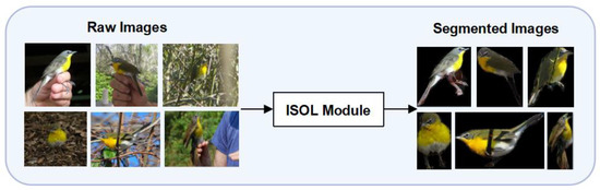
Figure 4. Instance-segmentation-based object localization (ISOL) module.

3.3. Graph-Based Multilevel Distribution Propagation

In this section, we will introduce the GMDP module in detail. As shown in Figure 5, the GMDP module consists of $l$ iterations, and each iteration consists of an object graph $G_l^{object}=\left(V_l^{object},E_l^{object}\right)$, a fist-level distribution graph $G_l^{dis{t}_1}=\left(V_l^{dis{t}_1},E_l^{dis{t}_1}\right)$, and a second-level distribution graph $G_l^{dis{t}_2}=\left(V_l^{dis{t}_2},E_l^{dis{t}_2}\right)$, and a third-level $G_l^{dis{t}_3}=\left(V_l^{dis{t}_3},E_l^{dis{t}_3}\right)$, the subscript $l$ means the $l\text{-}\mathrm{th}$ iterations. Firstly, the object feature $V_l^{object}$ was extracted from images by the backbone:

$$v_{0, i}^{object}=f_{emb}\left(x_i\right),$$

(1)

where $f_{emb}\left(x_i\right)$ is the backbone. As nodes in $G_l^{object}$, $V_l^{object}$ is used to calculate the edge feature $E_l^{object}$. Second, we fuse $E_l^{object}$ and $V_{l-1}^{dis{t}_1}$, which is the nodes of $G_{l-1}^{dis{t}_1}$, to get $V_l^{dis{t}_1}$, which are the nodes of $G_l^{dis{t}_1}$. $V_l^{dis{t}_1}$ is initialized in the order of $G_l^{object}$ and used to calculate the edge feature $E_l^{dis{t}_1}$, which represents the distribution of $V_l^{dis{t}_1}$, i.e., fist-level distribution; $E_l^{dis{t}_1}$ is then directly sent to construct the nodes $V_l^{dis{t}_2}$ in $G_l^{dis{t}_2}$. $V_l^{dis{t}_2}$ is initialized in the order of $G_l^{dis{t}_1}$ and is used to calculate $E_l^{dis{t}_2}$, which represents the distribution of $V_l^{dis{t}_2}$, i.e., second-level distribution; Similarly, $E_l^{dis{t}_2}$ are directly used to construct the nodes $V_l^{dis{t}_3}$ in $G_l^{dis{t}_3}$. $V_l^{dis{t}_3}$ is initialized in the order of $G_l^{dis{t}_2}$ and used to calculate $E_l^{dis{t}_3}$, which represents the distribution of node $V_l^{dis{t}_3}$, i.e., third-level distribution. Finally, these three levels of distribution $E_l^{dis{t}_1},E_l^{dis{t}_2},\mathrm{and}{E}_l^{dis{t}_3}$ will be used to update the object feature $V_l^{object}$ to produce a new node $V_{l+1}^{object}$, which are the nodes of the object graph $G_{l+1}^{object}$. This is one complete iteration.

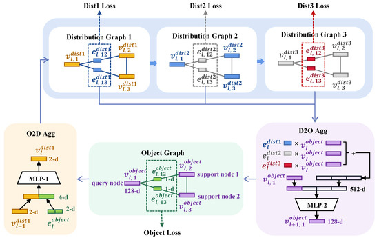
Figure 5. Details about MDPN. A 2 way-1 shot task is presented as an example. MLP-1 is the FC-ReLU blocks mentioned in O2D Aggregation and MLP-2 is the Conv-BN-ReLU blocks mentioned in D2O Aggregation.

$V_l^{object}, E_l^{object}, V_l^{dis{t}_1},E_l^{dis{t}_1},V_l^{dis{t}_2},E_l^{dis{t}_2},V_l^{dis{t}_3},E_l^{dis{t}_3}$ are defined as follows: $V_l^{object}$ = {$v_{l,i}^{object}$}, $E_l^{object}$ = {$e_{l,ij}^{object}$}, $V_l^{dis{t}_1}$ = {$v_{l,i}^{dis{t}_1}$},$E_l^{dis{t}_1}$ = {$e_{l,ij}^{dis{t}_1}$}, $V_l^{dis{t}_2}$ = {$v_{l,i}^{dis{t}_2}$},$E_l^{dis{t}_2}$ = {$e_{l,ij}^{dis{t}_2}$}, $V_l^{dis{t}_3}$ = {$v_{l,i}^{dis{t}_3}$},$E_l^{dis{t}_3}$ = {$e_{l,ij}^{dis{t}_3}$} where $i,j=1,\dots ,T$. $T=N\times K+\overline{T}$ denotes the total number of samples in a training episode, N × K denotes the number of support samples and $\overline{T}$ denotes the number of query samples.

Object Propagation. Each edge in the object’s graph stands for the object similarity. The edge $e_{l,ij}^{object}$ in the object graph represents the distribution of the object features, and $e_{0,ij}^{object}$ is updated as follows:

$$e_{0, ij}^{object}=\left\{\begin{array}{c}{f}_{e_0^{object}}\left({\left(v_{0, i}^{object}-v_{0, j}^{object}\right)}^2\right), l=0,\hfill \\ f_{ e_l^{object}}\left({\left(v_{l, i}^{object}-v_{l, j}^{object}\right)}^2\right). e_{l-1, ij}^{object}, l>0,\hfill \end{array}\right.$$

(2)

where $e_{0,ij}^{object}\in ℝ$. $f_{e_0^{object}}:{ℝ}^m\to ℝ$ is an encoding network that transforms a distribution into a metric. $f_{e_0^{object}}$ is made of two Conv-BN-ReLU [33,34] blocks and a sigmoid layer. Finally, a normalization operation is conducted on $e_{l,ij}^{object}$.

O2D Aggregation. The object-distribution aggregation integrates $E_l^{object}$ and $V_{l-1}^{dis{t}_1}$ to get $V_l^{dis{t}_1}$. $v_{0,i}^{dis{t}_1}$ is initialized as follows:

$$v_{0, i}^{dis{t}_1}=\left\{\begin{array}{c}|{|}_{j=1}^{N_{sup}}\delta \left(y_i, y_j\right), if x_i is labeled,\hfill \\ \left[\frac{1}{N_{sup}}, \dots , \frac{1}{N_{sup}}\right], otherwise,\hfill \end{array}\right.$$

(3)

where $v_{0,i}^{dis{t}_1}\in {ℝ}^{N_{sup}}$. || is the concatenation operator. $y_i$ and $y_j$ are labels. $\delta \left(·\right)$ is the Kronecker delta function, which outputs 1 when $y_i=y_j$, 0 otherwise.

When the iteration number $l>0$, $v_{l,i}^{dis{t}_1}$ is updated as follows:

$$v_{l, i}^{dis{t}_1}=O2D\left(\left|\right|{ }_{j=1}^{N_{sup}} e_{l, ij}^{object}, v_{l-1, i}^{dis{t}_1} \right),$$

(4)

where $O2D:\left({ℝ}^{N_{sup}},{ℝ}^{N_{sup}}\right)\to {ℝ}^{N_{sup}}$ is the object-distribution aggregation network. $O2D$ first connects two features together and then transforms it: ${ℝ}^{2N_{sup}}\to {ℝ}^{N_{sup}}$, this transformation contains a fully connected (FC) layer and a ReLU.

Distribution Propagation. The first-level distribution ${\mathit{e}}_{\mathit{l},\mathit{i}\mathit{j}}^{\mathit{d}\mathit{i}\mathit{s}{\mathit{t}}_{\mathit{1}}}$ is updated as follows:

$$e_{0, ij}^{dis{t}_1}=\left\{\begin{array}{c}{f}_{ e_0^{dis{t}_1}}\left({\left(v_{0, i}^{dis{t}_1}-v_{0, j}^{dis{t}_1}\right)}^2\right), l=0,\\ f_{ e_l^{dis{t}_1}}\left({\left(v_{l, i}^{dis{t}_1}-v_{l, j}^{dis{t}_1}\right)}^2\right). e_{l-1, ij}^{dis{t}_1}, l>0.\end{array}\right.$$

(5)

where $e_{0,ij}^{dis{t}_1}\in ℝ$. The encoding network $f_{e_0^{dis{t}_1}}:{ℝ}^{NK}\to {ℝ}^{NK}$ is composed of two Conv-BN-ReLU blocks. Finally, a normalization operation is conducted on $e_{l,ij}^{dis{t}_1}$. The edge of the first-level distribution $e_{0,ij}^{dis{t}_1}$ is directly used as a node of the second-level distribution: $e_{0,ij}^{dis{t}_1}=v_{0,i}^{dis{t}_2}$. Similarly in the third-level graph: $e_{0,ij}^{dis{t}_2}=v_{0,i}^{dis{t}_3}$. The second-level distribution $e_{l,ij}^{dis{t}_2}$ and the third-level distribution $e_{l,ij}^{dist\_3}$ are updated as follows:

$$e_{l, ij}^{dis{t}_2}=\left\{\begin{array}{c}{f}_{e_l^{dis{t}_2}}\left({\left(v_{l, i}^{dis{t}_2}-v_{l, j}^{dis{t}_2}\right)}^2\right), l=0,\\ f_{e_l^{dis{t}_2}}\left({\left(v_{l, i}^{dis{t}_2}-v_{l, j}^{dis{t}_2}\right)}^2\right)·e_{l-1, ij}^{dis{t}_2}, l>0.\end{array}\right.$$

(6)

$$e_{l,ij}^{dis{t}_3}=\left\{\begin{array}{c}{f}_{e_l^{dis{t}_3}}\left({\left(v_{l,i}^{dis{t}_3}-v_{l,j}^{dis{t}_3}\right)}^2\right), l=0,\\ f_{e_l^{dis{t}_3}}\left({\left(v_{l,i}^{dis{t}_3}-v_{l,j}^{dis{t}_3}\right)}^2\right) ·e_{l-1,ij}^{dis{t}_3}, l>0.\end{array}\right.$$

(7)

D2O Aggregation. In the D2O module, three levels of distributions: $e_{l,ij}^{dis{t}_1}$, $e_{l,ij}^{dis{t}_2}$, $e_{l,ij}^{dis{t}_3}$ are used to update the $v_{l,i}^{object}$ into $v_{l+1,i}^{object}$. $v_{l+1,i}^{object}$ is updated as follows:

$$v_l^{{\mathit{fuse}}_{\mathrm{x}}}={\displaystyle {{\displaystyle \sum }}_{j=1}^T}\left(e_{l,ij}^{dis{t}_{\mathrm{x}}}·v_{l,j}^{object}\right),x=\left\{1,2,3\right\},$$

(8)

$$v_l^{cat}=v_{l, i}^{object}\left|\left|v_l^{fus{e}_1}\right|\right|v_l^{fus{e}_2}\left|\right|v_l^{fus{e}_3},$$

(9)

$$v_{l+1, i}^{object}=D2O\left(v_l^{cat}\right),$$

(10)

where $v_{l,i}^{object}\in {ℝ}^m$, D2O:$\left({ℝ}^m,{ℝ}^m\right)\to {ℝ}^m$ is the distribution-object aggregation network. D2P consists of two Conv-BN-ReLU blocks. Benefiting from the aggregation, $v_{l+1,i}^{object}$ contains the multilevel distribution information.

3.4. Objective

The class prediction of each node in the object graph and in the three distribution graphs is calculated as follows:

$$P^{object}(y_j|x_{ i})=Softmax\left({{\displaystyle \sum }}_{j=1}^{NK}{e}_{l, ij}^{object}·one-hot\left(y_j\right)\right),$$

(11)

$$P^{dis{t}_x}\left(y_j|x_i\right)=Softmax\left({\displaystyle \sum }_{j=1}^{NK}{e}_{l,ij}^{dis{t}_x}·one\text{-}hot\left(y_j\right)\right),x=\left\{1,2,3\right\},$$

(12)

where $x_i$ is the query sample and $y_j$ is the label of $j\text{-}\mathrm{th}$ support sample. $P\left(y_j|x_i\right)$ is the probability distribution over classes given sample $x_i$. $e_{l,ij}^{object}$ and $e_{l,ij}^{dis{t}_x}$ are the edges connecting node $x_i$ and node $x_j$ in the $l\text{-}\mathrm{th}$ iteration (where $x_i$ is the query sample and $x_j$ is the support sample). $one\text{-}hot\left(y_j\right)$ is the one-hot encoding of the $y_j$.

Object Loss. The object loss is inherited from baseline(DPGN [26]):

$$L_l^{object}=L_{CE}\left(P^{object}\left(y_j|x_i\right), y_j\right),$$

(13)

where $L_{CE}$ is the cross-entropy loss function. $P^{object}\left(y_j|x_i\right)$ is calculated by (11).

Distribution Loss. The distribution loss in the $l\text{-}\mathrm{th}$ iteration is calculated as follows:

$$L_l^{dis{t}_x}=L_{CE}\left(P^{dis{t}_x}\left({\widehat{y}}_i|x_{ i}\right), y_i\right), x=\left\{1, 2, 3\right\},$$

(14)

$$L_l^{dist}={\lambda }_{dis{t}_1}{L}_l^{dis{t}_1}+{\lambda }_{dis{t}_2}{L}_l^{dis{t}_2}+{\lambda }_{dis{t}_3}{L}_l^{dis{t}_3}/N_{\lambda }, N_{\lambda }={{\displaystyle \sum }}_{x=\left\{1, 2, 3\right\}}\left({\lambda }_{dis{t}_x}!=0\right),$$

(15)

where $P^{dis{t}_x}\left(y_j|x_i\right)$ is calculated by (12). $L_l^{dis{t}_1}$, $L_l^{dis{t}_2}$, and $L_l^{dis{t}_3}$ are the three distribution losses. ${\lambda }_{dis{t}_1}$, ${\lambda }_{dis{t}_2}$, and ${\lambda }_{dis{t}_3}$ are the weight factors of the corresponding distribution loss. $\left[{\lambda }_{dis{t}_1},{\lambda }_{dis{t}_2},{\lambda }_{dis{t}_3}\right]=\left[0.0,0.0,1.0\right]$ in a 5-way 1-shot setting and $\left[{\lambda }_{dis{t}_1},{\lambda }_{dis{t}_2},{\lambda }_{dis{t}_3}\right]=\left[1.0,1.0,1.0\right]$ in a 5-way 5-shot setting. The reason for the setting of the weight factors will be explained in Section 4.

The objective function is made up of these two losses:

$$L={{\displaystyle \sum }}_{l=1}^{\widehat{l}}\left({\lambda }_{object}{L}_l^{object}+{\lambda }_{dist}{L}_l^{dist}\right),$$

(16)

where $\widehat{l}$ is the total number of iterations in the GMDP module. The two weight factors ${\lambda }_{object}$ and ${\lambda }_{dist}$ are used to measure the importance of the two losses. We follow the setting of the baseline: $\left[{\lambda }_{object},{\lambda }_{dist}\right]=\left[1.0,0.1\right]$.

4. Experiment

4.1. Dataset

We assess MDPN using the common benchmarks for few-shot learning, CUB-200-2011 [35]. A total of 200 bird species are represented by 11,788 photos in CUB-200-201, which is broken down into 100 base classes, 50 validation classes, and 50 novel classes.

4.2. Experiment Setups

Our experiment setting is consistent with the baseline to guarantee that our model is comparable to it.

Network Architecture. We use ResNet12 as the backbone. It mainly has four blocks, which include one residual block. The last feature of the backbone is processed by global average pooling, then goes through an FC layer with batch normalization (BN) to obtain a 128-dimensional object embedding as the final output of the backbone network.

Implementation Details. We perform data augmentation prior to training, e.g., horizontal flipping, random cropping, and color jitter (brightness, contrast, and saturation), as mentioned in [36,37]. We set the number of episodes to 28 in each epoch. In our experiments, we use the Adam optimizer with an initial learning rate of ${10}^{-3}$. The decay of the learning rate is set to 0.1 per 15,000 iterations and the weight decay to ${10}^{-5}$.

Evaluation Metrics. We evaluated MDPN in 5-way 1-shot and 5-way 5-shot settings on CUB-200-2011. Following the evaluation process of previous methods [25,37,38], we randomly sampled 10,000 tasks to calculate the mean accuracy with 95% confidence intervals as the final result. Our experiments are implemented in PyTorch.

Evaluation Metrics. The number of iterations in GMDP is chosen to be 6 as a trade-off between convergence time and accuracy.

4.3. Experiment Results

Main Results. We contrast MDPN’s performance with that of the well-known ProtoNet and the current top models, such as DeepEMD [39], FEAT [40], and FRN [41]. We tested the approach with the same dataset, CUB-200-2011, and backbone, ResNet12, for an accurate comparison. Table 1 demonstrates that MDPN outperforms the baseline (DPGN [26]) as well as the majority of the existing methods.

Table 1. The accuracy (%) of 5-way 1-shot and 5-way 5-shot settings on CUB-200-2011. The best outcomes are highlighted in bold.

Model	Backbone	CUB-200-2011
		5-Way 1-Shot	5-Way 5-Shot
ProtoNet [15] (2017) *	resnet12	66.09 ± 0.92	82.50 ± 0.58
cosine classifier [42] (2019) *	resnet12	67.30 ± 0.86	84.75 ± 0.60
MatchingNet [14] (2016) *	resnet12	71.87 ± 0.85	85.08 ± 0.57
FEAT [40] (2020) *	resnet12	73.27 ± 0.22	85.77 ± 0.14
DeepEMD [39] (2020) *	resnet12	75.65 ± 0.83	88.69 ± 0.50
DMN4 [43] (2022)	resnet12	82.95 ± 0.75	90.46 ± 0.46
RENet [44] (2021)	resnet12	79.49 ± 0.44	91.11 ± 0.24
DPGN [26] (2020)	resnet12	75.71 ± 0.47	91.48 ± 0.33
EPNet [45] (2020)	resnet12	82.85 ± 0.81	91.32 ± 0.41
ECKPN [46] (2021)	resnet12	77.43 ± 0.54	92.21 ± 0.41
FRN [41] (2021)	resnet12	82.12 ± 0.85	92.49 ± 0.43
MDPN (ours)	resnet12	83.55 ± 0.33	92.72 ± 0.17

* Denotes that is reported from [26].

5. Discussion

5.1. The Impact of ISOL

The localization method via the supervised learning-based attention mechanism, which is an inaccurate localization focusing on only part of the object region and losing other information, is substantially worse than our prior-knowledge-based ISOL. The accuracy and integrity of the location of the object region directly affect feature extraction and are also reflected in classification accuracy. We conducted a number of ablation experiments on CUB-200-2011 in 5-way 1-shot and 5-way 5-shot settings to demonstrate that our ISOL outperforms the non-localization approach and attention mechanism. The data in Table 2 demonstrates that, when compared to the other two methods, our MDPN, which is based on instance segmentation, has the highest accuracy. We choose CBAM for two reasons when evaluating the impact of attention mechanisms: (1) it is a plug-and-play module, and (2) it combines CAM and SAM [47]. CAM concentrates on channel, while SAM concentrates on spatial. CBAM can produce better results than CAM, Grad-CAM, and SENet [48], which exclusively concentrate on channels.

Table 2. The accuracy (%) of different localization methods in 5-way 1-shot and 5-way 5-shot settings on CUB-200-2011. The best outcomes are highlighted in bold. A0 denotes the MDPN without ISOL module. A1 denotes the MDPN, with CBAM replacing ISOL module. A2 denotes the MDPN, which contains ISOL module.

Model	ISOL	CBAM	CUB-200-2011
			5-Way 1-Shot	5-Way 5-Shot
A0			77.39	85.98
A1		√	77.84	86.37
A2 (ours)	√		83.55	92.72

5.2. The Impact of GMDP

We perform a series of ablation experiments on various stacking numbers of distribution propagation on CUB-200-2011 in 5-way 1-shot and 5-way 5-shot configurations to confirm the viability of GMDP. Table 3 demonstrates that when the degree of distribution propagation rises, the classification accuracy of MDPN steadily improves and peaks with a configuration of three levels.

Table 3. The accuracy (%) of distribution propagation with various numbers of levels in 5-way 1-shot and 5-way 5-shot settings on cub-200-2011. The best outcomes are highlighted in bold. B0 denotes one level of distribution propagation. B1 denotes two levels of distribution propagation. B2 denotes the MDPN, which contains three levels of distribution propagation. B3 denotes four levels of distribution propagation. B4 denotes five levels of distribution propagation.

Model	DP1	DP2	DP3	DP4	DP5	CUB-200-2011
						5-Way 1-Shot	5-Way 5-Shot
B0	√					82.92	90.58
B1	√	√				83.43	91.69
B2 (ours)	√	√	√			83.88	92.72
B3	√	√	√	√		83.71	92.34
B4	√	√	√	√	√	83.59	92.05

5.3. The Impact of Weight Factors

As mentioned in Section 3.4, we set the weight control factors ${\lambda }_{dist\_1}$, ${\lambda }_{dist\_2}$, ${\lambda }_{dist\_3}$, in (16) as follows: $\left[{\lambda }_{dist\_1},{\lambda }_{dist\_2},{\lambda }_{dist\_3}\right]=\left[0.0,0.0,1.0\right]$ in a 5-way 1-shot setting, and $\left[{\lambda }_{dist\_1},{\lambda }_{dist\_2},{\lambda }_{dist\_3}\right]=\left[1.0,1.0,1.0\right]$ in a 5-way 5-shot setting. In order to verify the effectiveness of the weight factors that we set to improve the classification accuracy, we conducted a series of experiments, as shown in Table 4.

Table 4. The accuracy (%) of different settings of three weight factors in the loss function in 5-way 1-shot and 5-way 5-shot settings on cub-200-2011. The best results are shown in bold. C0 denotes $\left[{\lambda }_{dis{t}_1},{\lambda }_{dis{t}_2},{\lambda }_{dis{t}_3}\right]=\left[0.0,0.0,1.0\right]$. C1 denotes $\left[{\lambda }_{dis{t}_1},{\lambda }_{dis{t}_2},{\lambda }_{dis{t}_3}\right]=\left[1.0,1.0,0.0\right]$. C2 denotes $\left[{\lambda }_{dis{t}_1},{\lambda }_{dis{t}_2},{\lambda }_{dis{t}_3}\right]=\left[1.0,1.0,1.0\right]$.

Model	${\mathit{\lambda }}_{\mathit{d}\mathit{i}\mathit{s}\mathit{t}\_1}$	${\mathit{\lambda }}_{\mathit{d}\mathit{i}\mathit{s}\mathit{t}\_2}$	${\mathit{\lambda }}_{\mathit{d}\mathit{i}\mathit{s}\mathit{t}\_3}$	CUB-200-2011
				5-Way 1-Shot	5-Way 5-Shot
C0	0.0	0.0	1.0	83.55 (ours)	85.03
C1	1.0	1.0	0.0	82.75	90.46
C2	1.0	1.0	1.0	80.66	92.72 (ours)

6. Conclusions

The MDPN proposed in this paper is optimized for the problems of noise interference and inadequate feature extraction in few-shot classification. The ISOL module dramatically reduces background and pseudo-object noise effects, and multilevel distributions are generated by the GMDP module. Benefiting from these, MDPN performs well on the CUB-200-2011: MDPN exceeds the baseline by 8.17% under the 5-way 1-shot setting and 1.24% under the 5-way 5-shot setting. For future work, we aim to validate our model on more small datasets.

References

- He, K.; Zhang, X.; Ren, S.; Sun, J. Deep residual learning for image recognition. In Proceedings of the IEEE Conference on Computer Vision and Pattern Recognition, Las Vegas, NV, USA, 27–30 June 2016; pp. 770–778. [Google Scholar]
- Krizhevsky, A.; Sutskever, I.; Hinton, G.E. Imagenet classification with deep convolutional neural networks. Commun. ACM 2017, 60, 84–90. [Google Scholar] [CrossRef]
- LeCun, Y.; Boser, B.; Denker, J.S.; Henderson, D.; DHoward, R.; Hubbard, W.; Jackel, L. Backpropagation applied to handwritten zip code recognition. Neural Comput. 1989, 1, 541–551. [Google Scholar] [CrossRef]
- Jiang, Z.; Kang, B.; Zhou, K.; Feng, J. Few-shot Classification via Adaptive Attention. arXiv 2020, arXiv:2008.02465. [Google Scholar]
- Santoro, A.; Bartunov, S.; Botvinick, M.; Wierstra, D.; Lillicrap, T. Meta-learning with memory-augmented neural networks. In Proceedings of the International Conference on Machine Learning PMLR, New York, NY, USA, 19–24 June 2016; pp. 1842–1850. [Google Scholar]
- Shi, X.; Chen, Z.; Wang, H.; Yeung, D.Y.; Wong, W.K.; Woo, W.C. Convolutional LSTM network: A machine learning approach for precipitation nowcasting. In Advances in Neural Information Processing Systems 28, Proceedings of the Annual Conference on Neural Information Processing Systems 2015, Montreal, Quebec, Canada, 7–12 December 2015; Cortes, C., Lawrence, N., Lee, D., Sugiyama, M., Garnett, R., Eds.; NeurIPS: San Diego, CA, USA, 2015; p. 28. [Google Scholar]
- Munkhdalai, T.; Yu, H. Meta networks. In Proceedings of the International Conference on Machine Learning PMLR, Sydney, NSW, Australia, 6–11 August 2017; pp. 2554–2563. [Google Scholar]
- Cai, Q.; Pan, Y.; Yao, T.; Yan, C.; Mei, T. Memory matching networks for one-shot image recognition. In Proceedings of the IEEE Conference on Computer Vision and Pattern Recognition, Salt Lake City, UT, USA, 18–23 June 2018; pp. 4080–4088. [Google Scholar]
- Kaiser, Ł.; Nachum, O.; Roy, A.; Bengio, S. Learning to remember rare events. arXiv 2017, arXiv:1703.03129. [Google Scholar]
- Finn, C.; Abbeel, P.; Levine, S. Model-agnostic meta-learning for fast adaptation of deep networks. In Proceedings of the International Conference on Machine Learning PMLR, Sydney, NSW, Australia, 6 August 2017; pp. 1126–1135. [Google Scholar]
- Li, Z.; Zhou, F.; Chen, F.; Li, H. Meta-sgd: Learning to learn quickly for few-shot learning. arXiv 2017, arXiv:1707.09835. [Google Scholar]
- Nichol, A.; Achiam, J.; Schulman, J. On first-order meta-learning algorithms. arXiv 2018, arXiv:1803.02999. [Google Scholar]
- Lee, K.; Maji, S.; Ravichandran, A.; Soatto, S. Meta-learning with differentiable convex optimization. In Proceedings of the IEEE/CVF Conference on Computer Vision and Pattern Recognition, Long Beach, CA, USA, 15–20 June 2019; pp. 10657–10665. [Google Scholar]
- Vinyals, O.; Blundell, C.; Lillicrap, T.; Kavukcuoglu, K.; Wierstra, D. Matching networks for one shot learning. In Advances in Neural Information Processing Systems, Proceedings of the 30th International Conference on Neural Information Processing Systems, Barcelona, Spain, 5–10 December 2016; NeurIPS: San Diego, CA, USA, 2016; p. 29. [Google Scholar]
- Snell, J.; Swersky, K.; Zemel, R. Prototypical networks for few-shot learning. In Advances in Neural Information Processing Systems, Proceedings of the 31st International Conference on Neural Information Processing Systems, Long Beach, CA, USA, 4–9 December 2017; NeurIPS: San Diego, CA, USA, 2017; p. 30. [Google Scholar]
- Sung, F.; Yang, Y.; Zhang, L.; Xiang, T.; Torr, P.H.S.; Hospedales, T.M. Learning to compare: Relation network for few-shot learning. In Proceedings of the IEEE Conference on Computer Vision and Pattern Recognition, San Juan, PR, USA, 17–19 June 2018; pp. 1199–1208. [Google Scholar]
- Zhu, Y.; Liu, C.; Jiang, S. Multi-attention Meta Learning for Few-shot Fine-grained Image Recognition. In Proceedings of the Twenty-Ninth International Joint Conference on Artificial Intelligence, Yokohama, Japan, 7–15 January 2021; pp. 1090–1096. [Google Scholar]
- Zhou, B.; Khosla, A.; Lapedriza, A.; Oliva, A.; Torralba, A. Learning deep features for discriminative localization. In Proceedings of the IEEE Conference on Computer Vision and Pattern Recognition, Las Vegas, NV, USA, 27–30 June 2016; pp. 2921–2929. [Google Scholar]
- Selvaraju, R.R.; Cogswell, M.; Das, A.; Vedantam, R.; Parikh, D.; Batra, D. Grad-cam: Visual explanations from deep networks via gradient-based localization. In Proceedings of the IEEE International Conference on Computer Vision, Las Vegas, NV, USA, 27–30 June 2017; pp. 618–626. [Google Scholar]
- Chattopadhay, A.; Sarkar, A.; Howlader, P.; Balasubramanian, V.N. Grad-cam++: Generalized gradient-based visual explanations for deep convolutional networks. In Proceedings of the 2018 IEEE Winter Conference on Applications of Computer Vision (WACV), Lake Tahoe, NV, USA, 12–15 March 2018; pp. 839–847. [Google Scholar]
- Woo, S.; Park, J.; Lee, J.Y.; Kweon, I.S. Cbam: Convolutional block attention module. In Proceedings of the European Conference on Computer Vision (ECCV), Munich, Germany, 8–14 September 2018; pp. 3–19. [Google Scholar]
- Gao, T.; Han, X.; Liu, Z.; Sun, M. Hybrid attention-based prototypical networks for noisy few-shot relation classification. Proc. AAAI Conf. Artif. Intell. 2019, 33, 6407–6414. [Google Scholar] [CrossRef]
- Garcia, V.; Bruna, J. Few-shot learning with graph neural networks. arXiv 2017, arXiv:1711.04043. [Google Scholar]
- Liu, Y.; Lee, J.; Park, M.; Kim, S.; Yang, E.; Hwang, S.; Yang, Y. Learning to propagate labels: Transductive propagation network for few-shot learning. arXiv 2018, arXiv:1805.10002. [Google Scholar]
- Kim, J.; Kim, T.; Kim, S.; Chang, D.Y. Edge-labeling graph neural network for few-shot learning. In Proceedings of the IEEE/CVF Conference on Computer Vision and Pattern Recognition, Long Beach, CA, USA, 15–20 June 2019; pp. 11–20. [Google Scholar]
- Yang, L.; Li, L.; Zhang, Z.; Zhou, X.; Zhou, E.; Liu, Y. Dpgn: Distribution propagation graph network for few-shot learning. In Proceedings of the IEEE/CVF Conference on Computer Vision and Pattern Recognition, Seattle, WA, USA, 13–19 June 2020; pp. 13390–13399. [Google Scholar]
- Gidaris, S.; Komodakis, N. Generating classification weights with gnn denoising autoencoders for few-shot learning. In Proceedings of the IEEE/CVF Conference on Computer Vision and Pattern Recognition, Long Beach, CA, USA, 15–20 June 2019; pp. 21–30. [Google Scholar]
- Zhang, Y.; Li, W.; Zhang, M.; Wang, S.; Tao, R.; Du, Q. Graph information aggregation cross-domain few-shot learning for hyperspectral image classification. IEEE Trans. Neural Netw. Learn. Syst. 2022, 1–14. [Google Scholar] [CrossRef] [PubMed]
- Zhong, X.; Gu, C.; Ye, M.; Huang, W.; Lin, C.W. Graph complemented latent representation for few-shot image classification. IEEE Trans. Multimed. 2022, 1. [Google Scholar] [CrossRef]
- Shalam, D.; Korman, S. The self-optimal-transport feature transform. arXiv 2022, arXiv:2204.03065. [Google Scholar]
- Hu, Y.; Pateux, S.; Gripon, V. Squeezing backbone feature distributions to the max for efficient few-shot learning. Algorithms 2022, 15, 147. [Google Scholar] [CrossRef]
- Zhang, H.; Cao, Z.; Yan, Z.; Zhang, C. Sill-net: Feature augmentation with separated illumination representation. arXiv 2021, arXiv:2102.03539. [Google Scholar]
- Ioffe, S.; Szegedy, C. Batch normalization: Accelerating deep network training by reducing internal covariate shift. In Proceedings of the International Conference on Machine Learning PMLR, Lille, France, 7–9 July 2015; pp. 448–456. [Google Scholar]
- Glorot, X.; Bordes, A.; Bengio, Y. Deep sparse rectifier neural networks. In Proceedings of the Fourteenth International Conference on Artificial Intelligence and Statistics, Fort Lauderdale, FL, USA, 11–13 April 2011; pp. 315–323. [Google Scholar]
- Wah, C.; Branson, S.; Welinder, P.; Perona, P.; Belongie, S. The Caltech-UCSD Birds-200–2011 Dataset; California Institute of Technology: Pasadena, CA, USA, 2011. [Google Scholar]
- Gidaris, S.; Komodakis, N. Dynamic few-shot visual learning without forgetting. In Proceedings of the IEEE Conference on Computer Vision and Pattern Recognition, Salt Lake City, UT, USA, 18–23 June 2018; pp. 4367–4375. [Google Scholar]
- Ye, H.J.; Hu, H.; Zhan, D.C.; Sha, F. Learning embedding adaptation for few-shot learning. arXiv 2018, arXiv:1812.03664. [Google Scholar]
- Rusu, A.A.; Rao, D.; Sygnowski, J.; Vinyals, O.; Pascanu, R.; Osindero, S.; Hadsell, R. Meta-learning with latent embedding optimization. arXiv 2018, arXiv:1807.05960,. [Google Scholar]
- Zhang, C.; Cai, Y.; Lin, G.; Shen, C. Deepemd: Few-shot image classification with differentiable earth mover’s distance and structured classifiers. In Proceedings of the IEEE/CVF Conference on Computer Vision and Pattern Recognition, Seattle, WA, USA, 13–19 June 2020; pp. 12203–12213. [Google Scholar]
- Ye, H.J.; Hu, H.; Zhan, D.C.; Sha, F. Few-shot learning via embedding adaptation with set-to-set functions. In Proceedings of the IEEE/CVF Conference on Computer Vision and Pattern Recognition, Seattle, WA, USA, 13–19 June 2020; pp. 8808–8817. [Google Scholar]
- Wertheimer, D.; Tang, L.; Hariharan, B. Few-shot classification with feature map reconstruction networks. In Proceedings of the IEEE/CVF Conference on Computer Vision and Pattern Recognition, Nashville, TN, USA, 20–25 June 2021; pp. 8012–8021. [Google Scholar]
- Chen, W.Y.; Liu, Y.C.; Kira, Z.; Wang, Y.C.F.; Huang, J.B. A closer look at few-shot classification. arXiv 2019, arXiv:1904.04232. [Google Scholar]
- Liu, Y.; Zheng, T.; Song, J.; Cai, D.; He, X. Dmn4: Few-shot learning via discriminative mutual nearest neighbor neural network. Proc. AAAI Conf. Artif. Intell. 2022, 36, 1828–1836. [Google Scholar] [CrossRef]
- Kang, D.; Kwon, H.; Min, J.; Cho, M. Relational embedding for few-shot classification. In Proceedings of the IEEE/CVF International Conference on Computer Vision, Montreal, QC, Canada, 10–17 October 2021; pp. 8822–8833. [Google Scholar]
- Rodríguez, P.; Laradji, I.; Drouin, A.; Lacoste, A. Embedding propagation: Smoother manifold for few-shot classification. In Computer Vision–ECCV 2020, Proceedings of the 16th European Conference, Part XXVI 16, Glasgow, UK, 23–28 August 2020; Springer International Publishing: Cham, Switzerland, 2020; pp. 121–138. [Google Scholar]
- Chen, C.; Yang, X.; Xu, C.; Huang, X.; Ma, Z. Eckpn: Explicit class knowledge propagation network for transductive few-shot learning. In Proceedings of the IEEE/CVF Conference on Computer Vision and Pattern Recognition, Nashville, TN, USA, 20–25 June 2021; pp. 6596–6605. [Google Scholar]
- Laskar, Z.; Kannala, J. Context aware query image representation for particular object retrieval. In Proceedings of the Image Analysis: 20th Scandinavian Conference, SCIA 2017, Tromsø, Norway, 12–14 June 2017; Springer International Publishing: Cham, Switzerland, 2017; pp. 88–99. [Google Scholar]
- Hu, J.; Shen, L.; Sun, G. Squeeze-and-excitation networks. In Proceedings of the IEEE Conference on Computer Vision and Pattern Recognition, Salt Lake City, UT, USA, 18–23 June 2018; pp. 7132–7141. [Google Scholar]
Disclaimer/Publisher’s Note: The statements, opinions and data contained in all publications are solely those of the individual author(s) and contributor(s) and not of MDPI and/or the editor(s). MDPI and/or the editor(s) disclaim responsibility for any injury to people or property resulting from any ideas, methods, instructions or products referred to in the content. |
© 2023 by the authors. Licensee MDPI, Basel, Switzerland. This article is an open access article distributed under the terms and conditions of the Creative Commons Attribution (CC BY) license (https://creativecommons.org/licenses/by/4.0/).