Reliability Inference of Multicomponent Stress–Strength System Based on Chen Distribution Using Progressively Censored Data

Abstract

In this paper, we study the inference of the multicomponent stress–strength reliability (MSSR) based on the Chen distribution using progressively Type-II censored data. Both the stress and strength variables follow the Chen distribution with a common second shape parameter. The maximum likelihood estimates and the asymptotic confidence intervals of the MSSR are developed. The bootstrap confidence interval of the MSSR is also constructed. The Bayesian estimation of the MSSR is obtained under the generalized entropy loss function using the Markov Chain Monte Carlo method. To check the effectiveness of the proposed approach, simulation studies are performed. Finally, a real data set is analyzed.

1. Introduction

Reliability estimation is a popular research topic that has recently received much attention. Many studies focus on the stress–strength system with two components, which can be regarded as two random variables X and Y, representing strength and stress. Its reliability is $R=P(X>Y)$. For this kind of system, extensive research has been carried out. Many scholars have discussed the estimation of this reliability under certain distributions, such as Weerahandi and Johnson [1], Badr et al. [2], Xu et al. [3], Hassan et al. [4], etc.

In the theory of reliability, the multicomponent stress–strength system is an extension of the classical stress–strength system, which contains one stress component and k independent strength components. The system will remain stable if at least s of the k strength values exceed the stress value. For instance, a bridge with k vertical cables that represent the strength of the structure is just a multicomponent stress–strength system. It will remain stable if the stress brought on by wind, high traffic volume, etc., does not exceed the values of at least s of its k strength components. Another example is an eight-cylinder vehicle engine, which operates as long as at least four of the eight cylinders are firing.

For k strengths that are exposed to one stress, strengths $X_1,X_2,...,X_k$ are independent random variables with the same cumulative distribution function (CDF) $F_X(y)$, and stress Y (independent of $X_1,X_2,...,X_k$) is a random variable with the CDF $F_Y(y)$. Then, the multicomponent stress–strength reliability (MSSR) can be described as

$$\begin{array}{cc}\hfill R_{s,k}& =P\left[\mathrm{at} \mathrm{least} s \mathrm{of} \left({\mathrm{X}}_1,{\mathrm{X}}_2,\dots ,{\mathrm{X}}_k\right) \mathrm{exceed} \mathrm{Y}\right]\hfill \\ \hfill & \hfill =\sum _{m=s}^k\left(\begin{array}{c}k\\ m\end{array}\right){\int }_{-\infty }^{+\infty }{\left[1-F_X(y)\right]}^m{\left[F_X(y)\right]}^{k-m}d{F}_Y(y).\end{array}$$

(1)

The estimation of the MSSR has been widely studied under complete sample data, where different distributions have been used. For example, Rao [5] studied the maximum likelihood estimation and asymptotic confidence interval of the MSSR based on generalized exponential distribution. Jia et al. [6] discussed the classical estimation of the MSSR based on generalized inverted exponential distribution. Nadar and Kizilaslan [7] derived the estimation of the MSSR based on the Marshall–Olkin Bivariate Weibull distribution using frequentist and Bayesian methods. The Bayesian estimators were developed using Lindley’s approximation and Markov Chain Monte Carlo techniques. Kizilaslan and Nadar [8] discussed the estimation of the MSSR based on the Bivariate Kumaraswamy distribution in a similar way.

Censoring is an effective tool that is often used in lifetime tests. In practical experiments, censoring plays an important role when there are not enough test units or when data for all test units cannot be collected because of the lack of time and resources. Type-I and Type-II censoring attract a lot of attention due to their mathematical simplicity. In Type-I censoring, if a pre-determined time is reached, the test will be stopped, whereas in Type-II censoring, if a pre-determined number of units fail, the test will be stopped. However, both censoring schemes may be inappropriate if the experimenter needs to intermittently remove units. Thus, progressive Type-II censoring is considered a better option and has been widely used in recent years. In this censoring, the intermittent removal of units is allowed. In addition, it saves time and expenses to a certain extent.

Progressive Type-II censoring in a lifetime test is as follows. Assume that M units are tested in the experiment. When the first failure $x_1$ happens, $R_1$ units are randomly removed. When the second failure $x_2$ happens, $R_2$ units are randomly removed, and so on. Finally, when the $m^{\mathrm{th}}$ failure $x_m$ happens, the remaining $R_m$ active units are all removed. Note that $M=R_1+R_2+...+R_m+m$. In this way, the ordered lifetime data for m elements are obtained using the censoring scheme $\{M,m,R_1,R_2,...,R_m\}$. This process is shown in Figure 1. In particular, progressive Type-II censoring can be seen as an extension of Type-II censoring, which is derived by assuming $R_i=0,i=1,2,...,m-1$. Otherwise, the complete sample is derived by assuming $R_i=0,i=1,2,...,m$.

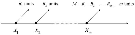
Figure 1. A schematic diagram of progressive Type-II censoring.

For samples that have been censored or are incomplete, there are few studies on the inference of the MSSR in the literature. Saini et al. [9] studied the estimation of the MSSR for Burr XII distribution using progressive first-failure censoring data. Tsai et al. [10] discussed the estimation of the MSSR for generalized exponential distribution using Type-I censoring data. Saini et al. [11] obtained the estimation of the MSSR for Topp–Leone distribution using progressive censoring data.

Many probability distributions have been proposed to fit the lifetime data. Here, we select the Chen distribution proposed by Chen [12]. Its probability density function (PDF), CDF, and hazard rate function (HRF) are, respectively, given by

$$f(x;\theta ,\lambda )=\theta \lambda x^{\lambda -1}exp\{x^{\lambda }+\theta (1-e^{x^{\lambda }})\},$$

(2)

$$F(x;\theta ,\lambda )=1-exp\{\theta (1-e^{x^{\lambda }})\},$$

(3)

$$h(x;\theta ,\lambda )=\theta \lambda x^{\lambda -1}exp\{x^{\lambda }\},$$

where $x>0$ and the shape parameters $\theta ,\lambda >0$. Hereafter, the Chen distribution can be represented by Chen$(\theta ,\lambda )$. Images of the PDFs and HRFs of the Chen distribution for certain cases are presented in Figure 2. It can be seen that the Chen distribution has a flexible PDF and HRF when the shape parameters are taken at different values. When $\lambda >1$, the PDFs have a significant peak; when $\lambda =1$, the PDFs have a roughly decreasing trend; and when $0<\lambda <1$, the PDFs are monotonically decreasing. Additionally, when $\lambda \ge 1$, the HRFs are monotonically increasing, and when $0<\lambda <1$, the HRFs present as a bathtub-shaped curve. In the literature, the Chen distribution has received considerable attention and has been studied by several scholars, including Chen and Gui [13], Rastogi et al. [14], Sarhan et al. [15], Mendez-Gonzalez et al. [16], and the references therein.

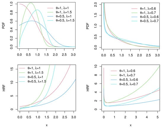
Figure 2. Images of PDFs and HRFs of Chen distribution under different sets of parameters.

Let $X_1,X_2,...,X_k$ follow $Chen({\theta }_1,\lambda )$ independently, and let Y (independent of $X_1,X_2,...,X_k$) follow $Chen({\theta }_2,\lambda )$. They have a common second shape parameter and different first shape parameters. Now, based on Equations (1)–(3), $R_{s,k}$ can be derived as

$$\begin{array}{cc}\hfill R_{s,k}& ={\theta }_2\lambda {\sum }_{m=s}^k\left(\begin{array}{c}k\\ m\end{array}\right){\int }_0^{\infty }{x}^{\lambda -1}exp\left\{\left(1-e^{x^{\lambda }}\right)\left({\theta }_{1}m+{\theta }_2\right)+x^{\lambda }\right\}{\left\{1-exp\left\{{\theta }_1\left(1-e^{x^{\lambda }}\right)\right\}\right\}}^{k-m}dx\hfill \\ & ={\theta }_2{\sum }_{m=s}^k\left(\begin{array}{c}k\\ m\end{array}\right){\sum }_{n=0}^{k-m}\left(\begin{array}{c}k-m\\ n\end{array}\right){(-1)}^n{\int }_1^{\infty }exp\left\{\left[{\theta }_1(m+n)+{\theta }_2\right](1-t)\right\}dt\hfill \\ \hfill & ={\sum }_{m=s}^k{\sum }_{n=0}^{k-m}\left(\begin{array}{c}k\\ m\end{array}\right)\left(\begin{array}{c}k-m\\ n\end{array}\right)\frac{{(-1)}^n{\theta }_2}{(m+n){\theta }_1+{\theta }_2},\hfill \end{array}$$

(4)

where $t=e^{x^{\lambda }}$.

As far as we know, no research has been conducted on the inference of the MSSR for the Chen distribution using progressively censored data. Wang et al. [17] discussed its classical estimation using Type-II censored data. So, our goal is to expand their research by carrying out its estimation from the Chen distribution using progressively censored data. In addition, the Bayesian estimation is also considered.

This article is organized as follows. In Section 2, the maximum likelihood estimate (MLE) is studied. Then, the interval estimation is discussed in Section 3. The asymptotic confidence interval (ACI) is derived based on the MLE. Additionally, the Bootstrap confidence interval (BootCI) is constructed. In Section 4, the Bayes estimates based on gamma priors are derived using the Markov Chain Monte Carlo (MCMC) method. The Bayesian credible interval (BCI) and the highest posterior density credible interval (HPDCI) are also discussed. In Section 5, Monte Carlo simulation studies are performed and a real data set is analyzed. Finally, the conclusions are reported in Section 6.

2. Maximum Likelihood Estimation

In this section, we derive the MLE of $R_{s,k}$ by adapting the approach of Wang et al. [17] and extending its application to progressively Type-II censored data. Assume that N systems with K strength components are subjected to a lifetime test. We observe the lifetime data for n systems with k components using progressive Type-II censoring. The observed $data$ $\underset{\sim }{x}$ and $\underset{\sim }{y}$ are described as follows:

                          Observed strength values       Observed stress values

$$\left(\begin{array}{cccc}{x}_{11}& x_{12}& \cdots & x_{1k}\\ ⋮& ⋮& \ddots & ⋮\\ x_{n1}& x_{n2}& \cdots & x_{nk}\end{array}\right)\hspace{1em}\hspace{1em}\mathrm{and}\hspace{1em}\hspace{1em}\left(\begin{array}{c}{y}_1\\ ⋮\\ y_n\end{array}\right)$$

where each row of values in $\underset{\sim }{x}$ is the censored sample from $Chen({\theta }_1,\lambda )$ with the progressive Type-II censoring scheme $\{K,k,S_1,S_2,...,S_k\}$, and $\underset{\sim }{y}$ is the censored sample from $Chen({\theta }_2,\lambda )$ with the progressive Type-II censoring scheme $\{N,n,T_1,T_2,...,T_n\}$. For simplicity, we denote the censoring scheme as $S=(S_1,S_2,...,S_k)$ and $T=(T_1,T_2,...,T_n)$. Then, the likelihood function is

$$L\left({\theta }_1,{\theta }_2,\lambda \right)=c_1\prod _{i=1}^n\left(c_2\prod _{j=1}^k{f}_X\left(x_{ij}\right){\left[1-F_X\left(x_{ij}\right)\right]}^{S_j}\right)f_Y\left(y_i\right){\left[1-F_Y\left(y_i\right)\right]}^{T_i},$$

(5)

where

$$c_1=N\left(N-T_1-1\right)\cdots \left(N-T_1-\cdots -S_{n-1}-n+1\right),$$

$$c_2=K\left(K-S_1-1\right)\cdots \left(K-S_1-\cdots -S_{k-1}-k+1\right).$$

Now, using Equations (2), (3), and (5), the likelihood function is

$$\begin{array}{cc}\hfill L({\theta }_1,{\theta }_2,\lambda )=& {\lambda }^{n(k+1)}{c}_1{c_2}^n{{\theta }_1}^{nk}{{\theta }_2}^n\prod _{i=1}^n\prod _{j=1}^k{x_{ij}}^{\lambda -1}exp\{{x_{ij}}^{\lambda }+{\theta }_1(1-e^{{x_{ij}}^{\lambda }})(1+S_j)\}\hfill \\ \hfill & \times \prod _{i=1}^n{y_i}^{\lambda -1}exp\{{y_i}^{\lambda }+{\theta }_2(1-e^{{y_i}^{\lambda }})(1+T_i)\}.\hfill \end{array}$$

(6)

From Equation (6), the log-likelihood function is

$$\begin{array}{cc}\hfill l=l({\theta }_1,{\theta }_2,\lambda )\propto & n(k+1)ln\lambda +nkln{\theta }_1+nln{\theta }_2\hfill \\ \hfill & +\sum _{i=1}^n\sum _{j=1}^k[(\lambda -1)ln{x}_{ij}+{x_{ij}}^{\lambda }+{\theta }_1(1-e^{{x_{ij}}^{\lambda }})(1+S_j)]\hfill \\ \hfill & +\sum _{i=1}^n[(\lambda -1)ln{y}_i+{y_i}^{\lambda }+{\theta }_2(1-e^{{y_i}^{\lambda }})(1+T_i)].\hfill \end{array}$$

(7)

By taking the derivative of $l({\theta }_1,{\theta }_2,\lambda )$ with respect to ${\theta }_1$ and ${\theta }_2$ and setting them to 0, we obtain the following equations:

$$\begin{array}{cc}\hfill \frac{\partial l}{\partial {\theta }_1}& \hfill =\frac{nk}{{\theta }_1}+\sum _{i=1}^n\sum _{j=1}^k(1-e^{{x_{ij}}^{\lambda }})(1+S_j)=0,\hfill \end{array}$$

(8)

$$\begin{array}{cc}\hfill \frac{\partial l}{\partial {\theta }_2}& \hfill =\frac{n}{{\theta }_2}+\sum _{i=1}^n(1-e^{{y_i}^{\lambda }})(1+T_i)=0.\hfill \end{array}$$

(9)

Using Equations (8) and (9), we derive

$$\widetilde{{\theta }_1}=\frac{nk}{{\sum }_{i=1}^n{\sum }_{j=1}^k(e^{{x_{ij}}^{\lambda }}-1)(1+S_j)},\widetilde{{\theta }_2}=\frac{n}{{\sum }_{i=1}^n(e^{{y_i}^{\lambda }}-1)(1+T_i)}.$$

(10)

Theorem 1.

For a given $\lambda >0$, the MLEs of ${\theta }_1$ and ${\theta }_2$ exist and are, respectively, given by $\widetilde{{\theta }_1}$ and $\widetilde{{\theta }_2}$ in Equation (10).

Proof. 

Let $t_i=\frac{{\theta }_i}{\widetilde{{\theta }_i}}$, $i=1,2$. Using inequality $ln{t}_i\le t_i-1$, we obtain

$$\begin{array}{cc}\hfill ln{\theta }_1& \le \frac{{\theta }_1}{nk}\sum _{i=1}^n\sum _{j=1}^k(e^{{x_{ij}}^{\lambda }}-1)(1+S_j)-1+ln\widetilde{{\theta }_1},\hfill \end{array}$$

(11)

$$\begin{array}{cc}\hfill ln{\theta }_2& \le \frac{{\theta }_2}{n}\sum _{i=1}^n(e^{{y_i}^{\lambda }}-1)(1+T_i)-1+ln\widetilde{{\theta }_2}.\hfill \end{array}$$

(12)

By substituting Equations (11) and (12) into (7), one obtains

$$\begin{array}{cc}\hfill l({\theta }_1,{\theta }_2,\lambda )\le & \hfill n(k+1)ln\lambda +nkln\widetilde{{\theta }_1}+nln\widetilde{{\theta }_2}-nk-n\\ \hfill & +\sum _{i=1}^n\sum _{j=1}^k[(\lambda -1)ln{x}_{ij}+{x_{ij}}^{\lambda }]\hfill \\ \hfill & +\sum _{i=1}^n[(\lambda -1)ln{y}_i+{y_i}^{\lambda }].\hfill \end{array}$$

From Equation (10), one obtains

$$nk=\widetilde{{\theta }_1}\sum _{i=1}^n\sum _{j=1}^k(e^{{x_{ij}}^{\lambda }}-1)(1+S_j),n=\widetilde{{\theta }_2}\sum _{i=1}^n(e^{{y_i}^{\lambda }}-1)(1+T_i).$$

One further obtains

$$\begin{array}{cc}\hfill l({\theta }_1,{\theta }_2,\lambda )\le & n(k+1)ln\lambda +nkln\widetilde{{\theta }_1}+nln\widetilde{{\theta }_2}\hfill \\ \hfill & +\sum _{i=1}^n\sum _{j=1}^k[(\lambda -1)ln{x}_{ij}+{x_{ij}}^{\lambda }+\widetilde{{\theta }_1}(1-e^{{x_{ij}}^{\lambda }})(1+S_j)]\hfill \\ \hfill & +\sum _{i=1}^n[(\lambda -1)ln{y}_i+{y_i}^{\lambda }+\widetilde{{\theta }_2}(1-e^{{y_i}^{\lambda }})(1+T_i)]\hfill \\ \hfill & =l(\widetilde{{\theta }_1},\widetilde{{\theta }_2},\lambda ).\hfill \end{array}$$

The equality holds if $t_i=1,i=1,2$, where ${\theta }_1=\widetilde{{\theta }_1}$ and ${\theta }_2=\widetilde{{\theta }_2}$.    □

From Theorem 1, by substituting ${\theta }_1=\widetilde{{\theta }_1}$ and ${\theta }_2=\widetilde{{\theta }_2}$ into Equation (7), the log-likelihood function of $\lambda$ is

$$\begin{array}{cc}\hfill l^{*}(\lambda )\propto & n(k+1)ln\lambda -nkln[\sum _{i=1}^n\sum _{j=1}^k(e^{{x_{ij}}^{\lambda }}-1)(1+S_j)]-nln[\sum _{i=1}^n(e^{{y_i}^{\lambda }}-1)(1+T_i)]\hfill \\ \hfill & +\sum _{i=1}^n\sum _{j=1}^k[(\lambda -1)ln{x}_{ij}+{x_{ij}}^{\lambda }]+\sum _{i=1}^n[ln{y}_i+{y_i}^{\lambda }ln{y}_i].\hfill \end{array}$$

(13)

By taking the derivative of $l^{*}(\lambda )$ and setting it to 0, we obtain the following equation and its solution is the MLE $\widehat{\lambda }$.

$$\begin{array}{cc}\hfill \frac{\mathrm{d}{l}^{*}}{\mathrm{d}\lambda }=& \frac{n(k+1)}{\lambda }-\frac{nk{\sum }_{i=1}^n{\sum }_{j=1}^k(1+S_j)e^{{x_{ij}}^{\lambda }}{x_{ij}}^{\lambda }ln{x}_{ij}}{{\sum }_{i=1}^n{\sum }_{j=1}^k(e^{{x_{ij}}^{\lambda }}-1)(1+S_j)}-\frac{n{\sum }_{i=1}^n(1+T_i)e^{{y_i}^{\lambda }}{y_i}^{\lambda }ln{y}_i}{{\sum }_{i=1}^n(e^{{y_i}^{\lambda }}-1)(1+T_i)}\hfill \\ \hfill & +\sum _{i=1}^n\sum _{j=1}^k(ln{x}_{ij}+{x_{ij}}^{\lambda }ln{x}_{ij})+\sum _{i=1}^n(ln{y}_i+{y_i}^{\lambda }ln{y}_i)=0.\hfill \end{array}$$

(14)

From Equation (14), we can derive a nonlinear equation $\beta (\lambda )=\lambda$, where

$$\begin{array}{cc}\hfill \beta (\lambda )=& n(k+1)[\frac{nk{\sum }_{i=1}^n{\sum }_{j=1}^k(1+S_j)e^{{x_{ij}}^{\lambda }}{x_{ij}}^{\lambda }ln{x}_{ij}}{{\sum }_{i=1}^n{\sum }_{j=1}^k(e^{{x_{ij}}^{\lambda }}-1)(1+S_j)}+\frac{n{\sum }_{i=1}^n(1+T_i)e^{{y_i}^{\lambda }}{y_i}^{\lambda }ln{y}_i}{{\sum }_{i=1}^n(e^{{y_i}^{\lambda }}-1)(1+T_i)}\hfill \\ \hfill & -\sum _{i=1}^n\sum _{j=1}^k(ln{x}_{ij}+{x_{ij}}^{\lambda }ln{x}_{ij})-\sum _{i=1}^n(ln{y}_i+{y_i}^{\lambda }ln{y}_i){]}^{-1}.\hfill \end{array}$$

(15)

The above equation has a fixed-point solution for $\lambda$. The MLE $\widehat{\lambda }$ can be derived using the fixed-point iterative approach as ${\lambda }_{(i+1)}=\beta ({\lambda }_{(i)})$, where ${\lambda }_{(i)}$ is the $i^{th}$ iterative value of $\lambda$. When $\left|{\lambda }_{(i+1)}-{\lambda }_{(i)}\right|$ is very close to 0, the iteration process can be stopped. Then, according to Equation (11), the MLEs $\widehat{{\theta }_1}$ and $\widehat{{\theta }_2}$ can be obtained using the MLE $\widehat{\lambda }$.

$$\widehat{{\theta }_1}=\frac{nk}{{\sum }_{i=1}^n{\sum }_{j=1}^k(e^{{x_{ij}}^{\widehat{\lambda }}}-1)(1+S_j)},\widehat{{\theta }_2}=\frac{n}{{\sum }_{i=1}^n(e^{{y_i}^{\widehat{\lambda }}}-1)(1+T_i)}.$$

(16)

Based on the invariance property of the MLEs, once we obtain the MLEs $\widehat{{\theta }_1}$, $\widehat{{\theta }_2}$, and $\widehat{\lambda }$, the MLE ${\widehat{R}}_{s,k}$ is

$${\widehat{R}}_{s,k}=\sum _{m=s}^k\sum _{n=0}^{k-m}\left(\begin{array}{c}\hfill k\hfill \\ \hfill m\hfill \end{array}\right)\left(\begin{array}{c}k-m\\ n\end{array}\right)\frac{{(-1)}^n\widehat{{\theta }_2}}{(m+n)\widehat{{\theta }_1}+\widehat{{\theta }_2}}.$$

(17)

3. Interval Estimation

3.1. Asymptotic Confidence Interval

Similar to the work of Wang et al. [17], we construct an ACI using the asymptotic normality of the MLE. Let $\widehat{\eta }=(\widehat{{\theta }_1},\widehat{{\theta }_2},\widehat{\lambda })$ be the MLEs of $\eta =({\theta }_1,{\theta }_2,\lambda )$. The observed Fisher information matrix is given by $I(\widehat{\eta })=[I_{ij}]={[-\frac{{\partial }^{2}l}{\partial {\eta }_i\partial {\eta }_j}]}_{\eta =\widehat{\eta }},i,j=1,2,3$, where

$$\begin{array}{cc}\hfill I_{11}=& \frac{nk}{{{\theta }_1}^2},I_{22}=\frac{n}{{{\theta }_2}^2},I_{12}=I_{12}=0,\hfill \\ \hfill I_{13}=& I_{31}=\sum _{i=1}^n\sum _{j=1}^k(1+S_j)e^{{x_{ij}}^{\lambda }}{x_{ij}}^{\lambda }ln{x}_{ij},I_{23}=I_{32}=\sum _{i=1}^n(1+T_i)e^{{y_i}^{\lambda }}{y_i}^{\lambda }ln{y}_i,\hfill \\ \hfill I_{33}=& \frac{n(k+1)}{{\lambda }^2}-\sum _{i=1}^n\sum _{j=1}^k[{x_{ij}}^{\lambda }{(ln{x}_{ij})}^2-{\theta }_1(1+S_j)e^{{x_{ij}}^{\lambda }}{x_{ij}}^{\lambda }{(ln{x}_{ij})}^2({x_{ij}}^{\lambda }+1)]\hfill \\ \hfill & -\sum _{i=1}^n[{y_i}^{\lambda }{(ln{y}_i)}^2-{\theta }_2(1+T_i)e^{{y_i}^{\lambda }}{y_i}^{\lambda }{(ln{y}_i)}^2({y_i}^{\lambda }+1)].\hfill \end{array}$$

Using the delta method (see Xu and Long [18]), the variance of ${\widehat{R}}_{s,k}$ is derived as follows:

$$Var({\widehat{R}}_{s,k})={(\frac{\partial R_{s,k}}{\partial {\theta }_1})}^2{[I^{-1}]}_{11}+{(\frac{\partial R_{s,k}}{\partial {\theta }_2})}^2{[I^{-1}]}_{22}+2(\frac{\partial R_{s,k}}{\partial {\theta }_1})(\frac{\partial R_{s,k}}{\partial {\theta }_2}){[I^{-1}]}_{12},$$

where

$$\begin{array}{cc}\hfill \frac{\partial R_{s,k}}{\partial {\theta }_1}& =\sum _{m=s}^k\sum _{n=0}^{k-m}\left(\begin{array}{c}\hfill k\hfill \\ \hfill m\hfill \end{array}\right)\left(\begin{array}{c}k-m\\ n\end{array}\right){(-1)}^{n+1}\frac{(m+n){\theta }_2}{{[(m+n){\theta }_1+{\theta }_2]}^2},\hfill \\ \hfill \frac{\partial R_{s,k}}{\partial {\theta }_2}& =\sum _{m=s}^k\sum _{n=0}^{k-m}\left(\begin{array}{c}\hfill k\hfill \\ \hfill m\hfill \end{array}\right)\left(\begin{array}{c}k-m\\ n\end{array}\right){(-1)}^n\frac{(m+n){\theta }_1}{{[(m+n){\theta }_1+{\theta }_2]}^2}.\hfill \end{array}$$

Here, the parameters $({\theta }_1,{\theta }_2,\lambda )$ are computed as the MLEs $(\widehat{{\theta }_1},\widehat{{\theta }_2},\widehat{\lambda })$. Therefore, the $100(1-\alpha )\%$ ACI for $R_{s,k}$ is

$$\left({\widehat{R}}_{s,k}-z_{\alpha /2}\sqrt{Var\left({\widehat{R}}_{s,k}\right)},{\widehat{R}}_{s,k}+z_{\alpha /2}\sqrt{Var\left({\widehat{R}}_{s,k}\right)}\right).$$

(18)

where $z_{\alpha }$ is $100(1-\alpha )th$ percentile of $N(0,1)$.

A negative lower bound might be generated by the ACI proposed above but $0<R_{s,k}<1$. To avoid this problem, the logit transformation can be used to provide a more accurate confidence interval, as proposed by Krishnamoorthy and Lin [19]. Let $\widehat{\xi }=ln({\widehat{R}}_{s,k}/(1-{\widehat{R}}_{s,k}))$ be the MLE of $\xi =ln(R_{s,k}/(1-R_{s,k}))$. Then, the $100(1-\alpha )\%$ ACI of $\xi$ is $({\xi }_L,{\xi }_U)$, where

$${\xi }_L=ln(\frac{{\widehat{R}}_{s,k}}{1-{\widehat{R}}_{s,k}})-z_{\alpha /2}\frac{\sqrt{Var({\widehat{R}}_{s,k})}}{{\widehat{R}}_{s,k}(1-{\widehat{R}}_{s,k})},$$

and

$${\xi }_U=ln(\frac{{\widehat{R}}_{s,k}}{1-{\widehat{R}}_{s,k}})+z_{\alpha /2}\frac{\sqrt{Var({\widehat{R}}_{s,k})}}{{\widehat{R}}_{s,k}(1-{\widehat{R}}_{s,k})}.$$

Then, the ACI of $R_{s,k}$ based on the logit scale is

$$(\frac{exp({\xi }_L)}{1+exp({\xi }_L)},\frac{exp({\xi }_U)}{1+exp({\xi }_U)}).$$

(19)

3.2. Bootstrap Confidence Interval

The MLEs may not follow the asymptotic normality when the observed sample size is insufficient, which can be a limitation of the ACI. Therefore, the BootCI is considered. Using the method discussed by Stine [20], the percentile BootCI is constructed. The procedures are provided in Algorithm 1.

Algorithm 1 The algorithm of the Bootstrap CI method.

Step 1 Obtain the MLEs $\widehat{{\theta }_1}$, $\widehat{{\theta }_2}$, and $\widehat{\lambda }$ with the given data sets $\underset{\sim }{x}$ and $\underset{\sim }{y}$ using the method mentioned in Section 2. Step 2 For a fixed progressive censoring scheme $(S_1,S_2,...,S_k)$, generate censored samples ${x_{i1}}^{*}$, ${x_{i2}}^{*}$, ..., ${x_{ik}}^{*}$ from $Chen(\widehat{{\theta }_1},\widehat{\lambda })$, $i=1,2,...,n$. Similarly, for a fixed progressive censoring scheme $(T_1,T_2,...,T_n)$, generate censored samples ${y_1}^{*}$, ${y_2}^{*}$, ..., ${y_n}^{*}$ from $Chen(\widehat{{\theta }_2},\widehat{\lambda })$. Step 3 Compute the MLE ${\widehat{R}}_{s,k}$ based on the samples in Step 2. Step 4 Repeat Steps 2–3 B times and obtain the ordered values $\tilde{R}(1)\le \tilde{R}(2)\le ...\le \tilde{R}(B)$. Step 5 The $100(1-\alpha )\%$ BootCI is given by $$(\tilde{R}([B\alpha /2]),\tilde{R}([B(1-\alpha /2)])),$$ where $[x]$ is the least integer function.

4. Bayesian Estimation

In this section, Bayesian estimation is discussed, together with the generalized entropy loss function (GELF). When overestimation and underestimation are considered different consequences of errors, the GELF is useful. The GELF is a suitable loss function used for reliability estimation since overestimating is typically considerably more harmful than underestimating. As first discussed by Calabria and Pulcini [21], the GELF is given by

$$L(\alpha ,\widehat{\alpha })\propto [{(\frac{\widehat{\alpha }}{\alpha })}^q-qln(\frac{\widehat{\alpha }}{\alpha })-1];q\ne 0,$$

where $\widehat{\alpha }$ is the decision rule to estimate $\alpha$. The Bayes estimate with the GELF is derived as

$$\widehat{\alpha }={[E({\alpha }^{-q}|data)]}^{-1/q}.$$

(20)

Note that the Bayes estimate in Equation (20) corresponds to the Bayes estimate with a precautionary loss function when $q=-2$, a squared error loss function when $q=-1$, and an entropy loss function when $q=1$.

In Bayesian estimation, ${\theta }_1$, ${\theta }_2$, and $\lambda$ can be considered random variables. Assume that they have independent gamma priors and their PDFs are expressed as follows:

$$g_1({\theta }_1)\propto {{\theta }_1}^{a_1-1}{e}^{-b_1{\theta }_1},{\theta }_1>0,$$

$$g_2({\theta }_2)\propto {{\theta }_2}^{a_2-1}{e}^{-b_2{\theta }_2},{\theta }_2>0,$$

$$g_3(\lambda )\propto {\lambda }^{a_3-1}{e}^{-b_3\lambda },\lambda >0,$$

where $a_i,b_i>0,i=1,2,3$. Then, the joint posterior density function is

$$\pi ({\theta }_1,{\theta }_2,\lambda |data)=\frac{L(data|{\theta }_1,{\theta }_2,\lambda )g_1({\theta }_1)g_2({\theta }_2)g_3(\lambda )}{{\int }_0^{\infty }{\int }_0^{\infty }{\int }_0^{\infty }L(data|{\theta }_1,{\theta }_2,\lambda )g_1({\theta }_1)g_2({\theta }_2)g_3(\lambda )d{\theta }_{1}d{\theta }_{2}d\lambda }.$$

(21)

By substituting Equation (6) into Equation (21), the posterior distribution is

$$\begin{array}{cc}\hfill \pi ({\theta }_1,{\theta }_2,\lambda |data)\propto & {{\theta }_1}^{nk+a_1-1}{{\theta }_2}^{n+a_2-1}{\lambda }^{n(k+1)+a_3-1}{e}^{-(b_1{\theta }_1+b_2{\theta }_2+b_3\lambda )}\hfill \\ \hfill & \times \prod _{i=1}^n\prod _{j=1}^k{x_{ij}}^{\lambda -1}exp\{{x_{ij}}^{\lambda }+{\theta }_1(1-e^{{x_{ij}}^{\lambda }})(1+S_j)\}\hfill \\ & \times \prod _{i=1}^n{y_i}^{\lambda -1}exp\{{y_i}^{\lambda }+{\theta }_2(1-e^{{y_i}^{\lambda }})(1+T_i)\}.\hfill \end{array}$$

(22)

4.1. MCMC Method

The MCMC method is considered to obtain the Bayesian estimation. According to Equation (22), the conditional posterior density of ${\theta }_1$, ${\theta }_2$, and $\lambda$ are derived as

$$\begin{array}{cc}\hfill {\theta }_1|\lambda ,data& \sim gamma(nk+a_1,b_1+\sum _{i=1}^n\sum _{j=1}^k(e^{{x_{ij}}^{\lambda }}-1)(1+S_j)),\hfill \\ \hfill {\theta }_2|\lambda ,data& \sim gamma(n+a_2,b_2+\sum _{i=1}^n(e^{{y_i}^{\lambda }}-1)(1+T_i)),\hfill \end{array}$$

and

$$\begin{array}{cc}\hfill {\pi }_1(\lambda |{\theta }_1,{\theta }_2,data)\propto & {\lambda }^{n(k+1)+a_3-1}{e}^{-b_3\lambda }\prod _{i=1}^n\prod _{j=1}^k{x_{ij}}^{\lambda }exp\{{x_{ij}}^{\lambda }+{\theta }_1(1-e^{{x_{ij}}^{\lambda }})(1+S_j)\}\hfill \\ \hfill & \times \prod _{i=1}^n{y_i}^{\lambda }exp\{{y_i}^{\lambda }+{\theta }_2(1-e^{{y_i}^{\lambda }})(1+T_i)\}.\hfill \end{array}$$

Now, using the gamma distributions, the values of ${\theta }_1$ and ${\theta }_2$ can be directly generated. Nonetheless, the Metropolis–Hastings (M–H) algorithm is utilized to obtain the values of $\lambda$. The procedure of the Gibbs sampling is provided in Algorithm 2. Then, according to the sampling results, the Bayes estimate with the GELF is

$${\widehat{R}}_{s,k}^{MC}={[\frac{1}{T-T_0}\sum _{t=T_0+1}^T{(R_{s,k}^{(t)})}^{-q}]}^{-1/q},$$

(23)

where $T_0$ is the burn-in period.

Algorithm 2 The algorithm of the MCMC method.

Step 1 Set the initial values ${{\theta }_1}^{(0)}$, ${{\theta }_2}^{(0)}$, and ${\lambda }^{(0)}$. Step 2 Set $t=1$. Step 3 Using the M–H algorithm, ${\lambda }^{(t)}$ can be generated from ${\pi }_1(\lambda |{{\theta }_1}^{(t-1)},{{\theta }_2}^{(t-1)},data)$. Here, the $N({\lambda }^{(t-1)},1)$ is used as the proposal distribution. Step 4 Obtain ${{\theta }_1}^{(t)}$ from $gamma(nk+a_1,b_1+{\sum }_{i=1}^n{\sum }_{j=1}^k(e^{{x_{ij}}^{{\lambda }^{(t-1)}}}-1)(1+S_j))$. Step 5 Obtain ${{\theta }_2}^{(t)}$ from $gamma(n+a_2,b_2+{\sum }_{i=1}^n(e^{{y_i}^{{\lambda }^{(t-1)}}}-1)(1+T_i))$. Step 6 Compute $R_{s,k}^{(t)}$ using ${{\theta }_1}^{(t)}$ and ${{\theta }_2}^{(t)}$. Step 7 Set $t=t+1$. Step 8 Repeat Steps 3-7 T times.

4.2. Bayesian Credible Intervals and Highest Posterior Density Credible Intervals

In this subsection, the BCI and HPDCI are constructed in the following way:

To begin with, the generated posterior samples $R_{s,k}^{(t)},t=T_0+1,T_0+2,...,T$ are sorted to derive the values $R_{(1)}\le R_{(2)}\le ...\le R_{(T-T_o)}$. Then, the BCI with a $100(1-\alpha )\%$ confidence level for $R_{s,k}$ is obtained as

$$(R_{([(T-T_0)(\alpha /2)])},R_{([(T-T_0)(1-\alpha /2)])}).$$

Among all the possible intervals with a $100(1-\alpha )\%$ confidence level, the HPDCI has the shortest width. Thus, the HPDCI for $R_{s,k}$ is given by

$$(R_{(n)},R_{(n+[(T-T_0)(1-\alpha )])}),$$

where n is the integer that makes

$$R_{(n+[(T-T_0)(1-\alpha )])}-R_{(n)}=\underset{1\le n\le T-T_0}{min}{R}_{(n+[(T-T_0)(1-\alpha )])}-R_{(n)},$$

where $[x]$ is the least integer function.

5. Numerical Explorations

5.1. Simulation Studies

To analyze the effects of various estimates, Monte Carlo simulations are performed. First, the samples with the censoring scheme $\{N,n,S_1,S_2,...,S_n\}$ are generated according to Algorithm 3, as discussed by Balakrishnan and Sandhu [22].

Algorithm 3 The algorithm for generating progressively censored samples.

Step 1 Obtain n independent random variables $W_1,W_2,...,W_n$ from the $Uniform(0,1)$ distribution. Step 2 Set $V_i=W_i^{1/{\sum }_{j=n-i+1}^n\left(S_j+1\right)}$, $i=1,2,...,n$. Step 3 Obtain $U_i=1-{\prod }_{j=n-i+1}^n{V}_j$, $i=1,2,...,n$, and thus $(U_1,U_2,...,U_n)$ are the required censored samples from the $Uniform(0,1)$ distribution. Step 4 Let $X_i=F^{-1}(U_i)$ for $i=1,2,...,n$, and then $(X_1,X_2,...,X_n)$ are the required progressively censored samples for the required distribution with CDF $F(x)$, where $F^{-1}(x)$ is its inverse function.

For the different point estimates, including MLEs and Bayes estimates, we compute their corresponding mean absolute deviations and mean squared errors. For different interval estimates, including 95% ACIs, BootCIs, BCIs, and HPDCIs, we compute their corresponding average lengths and coverage probabilities.

The various progressive Type-II censoring schemes (C.S) selected for the simulations are shown in Table 1, where $S_1$, $S_2$, ..., $S_6$ are the censoring schemes used for the strength variables, and $T_1$, $T_2$, ..., $T_6$ are the censoring schemes used for the stress variables. We perform lifetime tests on N systems with K components and observe the data obtained for n systems with k components using a certain censoring scheme. For simplicity, a short notation such as ($1\times 3$) represents (1, 1, 1) and ($(0,1)\times 3$) represents (0, 1, 0, 1, 0, 1). Take $s=3$ in schemes $S_1$, $S_2$, and $S_3$ and $s=2$ in schemes $S_4$, $S_5$, and $S_6$. When at least two or three components survive, we derive the estimations of the system reliability. The simulation results are based on 3000 replications and all simulation calculations are performed using R-4.3.0 software.

Table 1. Different censoring schemes.

(k, K)		C.S	(n, N)		C.S
(5, 15)	$S_1$	($0\times 4$, 10)	(10, 15)	$T_1$	($0\times 9$, 5)
	$S_2$	(10, $0\times 4$)		$T_2$	(5, $0\times 9$)
	$S_3$	($2\times 5$)		$T_3$	($(0,1)\times 5$)
(4, 10)	$S_4$	(0, 0, 0, 6)	(15, 30)	$T_4$	($0\times 14$, 15)
	$S_5$	(6, 0, 0, 0)		$T_5$	(15, $0\times 14$)
	$S_6$	(2, 2, 1, 1)		$T_6$	($1\times 15$)

Here, two different sets of distribution parameters are used:

$${\eta }_1=({\theta }_1,{\theta }_2,\lambda )=(1,1,2),{\eta }_2=({\theta }_1,{\theta }_2,\lambda )=(1.5,2,2).$$

For ${\eta }_1$, $R_{3,5}$ is 0.5 and $R_{2,4}$ is 0.6, whereas for ${\eta }_2$, $R_{3,5}$ is 0.5901 and $R_{2,4}$ is 0.6885.

To compute the Bayesian estimates, three priors are considered. The non-informative prior is denoted as prior 1 and the gamma priors are denoted as prior 2 for ${\eta }_1$ and prior 3 for ${\eta }_2$. The relevant parameters for the priors are as follows:

$$\begin{array}{cc}\hfill & \mathrm{Prior}1:a_i=b_i=0,i=1,2,3.\hfill \\ \hfill & \mathrm{Prior}2:a_1=1,b_1=1,a_2=1,b_2=1,a_3=2,b_3=1.\hfill \\ \hfill & \mathrm{Prior}3:a_1=3,b_1=2,a_2=2,b_2=1,a_3=2,b_3=1.\hfill \end{array}$$

For the GELF, three loss functions are considered:

$$\begin{array}{cc}\hfill & \mathrm{F}1:\mathrm{squared}\mathrm{error}\mathrm{loss}\mathrm{function} (q=-1)\hfill \\ \hfill & \mathrm{F}2:\mathrm{entropy}\mathrm{loss}\mathrm{function} (q=1)\hfill \\ \hfill & \mathrm{F}3:\mathrm{precautionary}\mathrm{loss}\mathrm{function} (q=-2)\hfill \end{array}$$

For two different sets of parameters and multiple combinations of censoring schemes, we obtain the MLEs and Bayes estimates. Then, we compute their mean absolute deviations (MAD) and mean squared errors (MSE), as shown in Table 2 for ${\eta }_1$ and Table 3 for ${\eta }_2$. The ACIs, BootCIs, BCIs, and HPDCIs for $R_{s,k}$ at a 95% confidence level are also derived under the same combinations of censoring schemes for two different sets of parameters. When computing the BootCIs, we take $B=1000$ re-samples. The average lengths (AL) and the coverage probabilities (CP) for different types of intervals are shown in Table 4 for ${\eta }_1$, and Table 5 for ${\eta }_2$.

Table 2. MADs and MSEs of the point estimations for ${\eta }_1$ when $R_{3,5}$ is 0.5 and $R_{2,4}$ is 0.6.

					Bayes
		MLE			Prior 1		Prior2
${\mathbf{\eta }}_{\mathbf{i}}$	C.S	MAD	MSE	GELF	MAD	MSE	MAD	MSE
${\eta }_1$	($S_1$, $T_1$)	0.0894	0.0121	F1	0.0853	0.0110	0.0781	0.0092
				F2	0.0905	0.0124	0.0829	0.0104
				F3	0.0841	0.0107	0.0771	0.0090
	($S_2$, $T_2$)	0.0886	0.0124	F1	0.0843	0.0112	0.0773	0.0094
				F2	0.0877	0.0120	0.0802	0.0100
				F3	0.0843	0.0112	0.0773	0.0094
	($S_3$, $T_3$)	0.0890	0.0127	F1	0.0852	0.0115	0.0781	0.0096
				F2	0.0908	0.0126	0.0833	0.0106
				F3	0.0839	0.0113	0.0770	0.0095
	($S_4$, $T_1$)	0.0971	0.0144	F1	0.0924	0.0131	0.0844	0.0110
				F2	0.0984	0.0151	0.0898	0.0126
				F3	0.0907	0.0126	0.0830	0.0105
	($S_5$, $T_2$)	0.0905	0.0125	F1	0.0868	0.0115	0.0798	0.0097
				F2	0.0928	0.0130	0.0852	0.0110
				F3	0.0850	0.0111	0.0782	0.0093
	($S_6$, $T_3$)	0.0889	0.0124	F1	0.0855	0.0115	0.0786	0.0097
				F2	0.0933	0.0135	0.0856	0.0114
				F3	0.0833	0.0109	0.0766	0.0092
	($S_1$, $T_4$)	0.0723	0.0084	F1	0.0701	0.0078	0.0659	0.0068
				F2	0.0729	0.0082	0.0685	0.0073
				F3	0.0695	0.0077	0.0653	0.0068
	($S_2$, $T_5$)	0.0682	0.0073	F1	0.0662	0.0069	0.0627	0.0062
				F2	0.0682	0.0073	0.0645	0.0065
				F3	0.0661	0.0069	0.0626	0.0062
	($S_3$, $T_6$)	0.0691	0.0075	F1	0.0669	0.0070	0.0633	0.0062
				F2	0.0697	0.0074	0.0659	0.0066
				F3	0.0664	0.0069	0.0628	0.0061
	($S_4$, $T_4$)	0.0733	0.0084	F1	0.0708	0.0078	0.0666	0.0069
				F2	0.0739	0.0085	0.0695	0.0075
				F3	0.0700	0.0077	0.0658	0.0068
	($S_5$, $T_5$)	0.0708	0.0079	F1	0.0691	0.0075	0.0656	0.0068
				F2	0.0725	0.0083	0.0688	0.0075
				F3	0.0680	0.0073	0.0646	0.0066
	($S_6$, $T_6$)	0.0746	0.0085	F1	0.0722	0.0080	0.0683	0.0071
				F2	0.0754	0.0087	0.0712	0.0078
				F3	0.0713	0.0078	0.0674	0.0069

Table 3. MADs and MSEs of the point estimations for ${\eta }_2$ when $R_{3,5}$ is 0.5901 and $R_{2,4}$ is 0.6885.

					Bayes
		MLE			Prior 1		Prior 3
${\mathbf{\eta }}_{\mathbf{i}}$	C.S	MAD	MSE	GELF	MAD	MSE	MAD	MSE
${\eta }_2$	($S_1$, $T_1$)	0.0888	0.0121	F1	0.0852	0.0112	0.0719	0.0080
				F2	0.0921	0.0130	0.0775	0.0092
				F3	0.0833	0.0107	0.0704	0.0076
	($S_2$, $T_2$)	0.0890	0.0123	F1	0.0855	0.0113	0.0723	0.0081
				F2	0.0914	0.0127	0.0771	0.0091
				F3	0.0839	0.0110	0.0711	0.0078
	($S_3$, $T_3$)	0.0904	0.0125	F1	0.0867	0.0115	0.0736	0.0083
				F2	0.0928	0.0130	0.0786	0.0094
				F3	0.0849	0.0110	0.0721	0.0080
	($S_4$, $T_1$)	0.0903	0.0125	F1	0.0877	0.0119	0.0737	0.0084
				F2	0.0955	0.0141	0.0799	0.0100
				F3	0.0849	0.0111	0.0716	0.0079
	($S_5$, $T_2$)	0.0807	0.0102	F1	0.0779	0.0096	0.0662	0.0070
				F2	0.0847	0.0114	0.0716	0.0082
				F3	0.0758	0.0091	0.0646	0.0066
	($S_6$, $T_3$)	0.0861	0.0114	F1	0.0833	0.0107	0.0703	0.0076
				F2	0.0901	0.0125	0.0758	0.0089
				F3	0.0809	0.0101	0.0684	0.0072
	($S_1$, $T_4$)	0.0697	0.0076	F1	0.0678	0.0072	0.0599	0.0056
				F2	0.0712	0.0078	0.0631	0.0061
				F3	0.0667	0.0070	0.0591	0.0055
	($S_2$, $T_5$)	0.0700	0.0076	F1	0.0681	0.0072	0.0613	0.0058
				F2	0.0708	0.0077	0.0637	0.0062
				F3	0.0673	0.0071	0.0606	0.0057
	($S_3$, $T_6$)	0.0715	0.0079	F1	0.0693	0.0074	0.0615	0.0058
				F2	0.0723	0.0080	0.0641	0.0063
				F3	0.0684	0.0073	0.0608	0.0057
	($S_4$, $T_4$)	0.0690	0.0073	F1	0.0669	0.0069	0.0590	0.0054
				F2	0.0701	0.0076	0.0618	0.0059
				F3	0.0658	0.0067	0.0580	0.0052
	($S_5$, $T_5$)	0.0630	0.0063	F1	0.0618	0.0060	0.0557	0.0049
				F2	0.0652	0.0066	0.0586	0.0054
				F3	0.0606	0.0058	0.0546	0.0047
	($S_6$, $T_6$)	0.0687	0.0073	F1	0.0669	0.0070	0.0593	0.0055
				F2	0.0704	0.0078	0.0623	0.0062
				F3	0.0658	0.0068	0.0583	0.0053

Table 4. ALs and CPs of the intervals for ${\eta }_1$ when $R_{3,5}$ is 0.5 and $R_{2,4}$ is 0.6.

						Bayes
						Prior 1		Prior 2
${\mathbf{\eta }}_{\mathbf{i}}$	C.S	AL/CP	ACI	Logit	BootCI	BCI	HPDCI	BCI	HPDCI
${\eta }_1$	($S_1$, $T_1$)	AL	0.4148	0.3936	0.4199	0.4003	0.3969	0.3885	0.3855
		CP	0.9227	0.9480	0.9260	0.9533	0.9360	0.9633	0.9487
	($S_2$, $T_2$)	AL	0.4065	0.3865	0.4053	0.3934	0.3898	0.3803	0.3775
		CP	0.9127	0.9413	0.9173	0.9400	0.9227	0.9560	0.9353
	($S_3$, $T_3$)	AL	0.4113	0.3906	0.4130	0.3974	0.3941	0.3853	0.3822
		CP	0.9133	0.9467	0.9260	0.9467	0.9247	0.9560	0.9400
	($S_4$, $T_1$)	AL	0.4216	0.4008	0.4246	0.4089	0.4039	0.3973	0.3928
		CP	0.9107	0.9473	0.9267	0.9453	0.9227	0.9567	0.9413
	($S_5$, $T_2$)	AL	0.4152	0.3956	0.4127	0.4039	0.3986	0.3917	0.3871
		CP	0.9100	0.9480	0.9353	0.9420	0.9207	0.9627	0.9353
	($S_6$, $T_3$)	AL	0.4171	0.3972	0.4187	0.4058	0.4002	0.3937	0.3888
		CP	0.9027	0.9447	0.9420	0.9460	0.9207	0.9573	0.9353
	($S_1$, $T_4$)	AL	0.3375	0.3257	0.3413	0.3298	0.3274	0.3221	0.3202
		CP	0.9300	0.9493	0.9367	0.9487	0.9360	0.9587	0.9427
	($S_2$, $T_5$)	AL	0.3256	0.3148	0.3261	0.3184	0.3163	0.3112	0.3092
		CP	0.9300	0.9493	0.9373	0.9487	0.9360	0.9513	0.9453
	($S_3$, $T_6$)	AL	0.3373	0.3254	0.3392	0.3294	0.3273	0.3216	0.3198
		CP	0.9220	0.9473	0.9393	0.9460	0.9287	0.9560	0.9420
	($S_4$, $T_4$)	AL	0.3454	0.3335	0.3450	0.3386	0.3354	0.3309	0.3277
		CP	0.9387	0.9540	0.9287	0.9587	0.9413	0.9613	0.9513
	($S_5$, $T_5$)	AL	0.3348	0.3239	0.3325	0.3285	0.3253	0.3214	0.3185
		CP	0.9167	0.9413	0.9300	0.9407	0.9233	0.9480	0.9373
	($S_6$, $T_6$)	AL	0.3446	0.3329	0.3426	0.3378	0.3345	0.3302	0.3273
		CP	0.9293	0.9473	0.9293	0.9493	0.9267	0.9547	0.9433

Table 5. ALs and CPs of the intervals for ${\eta }_2$ when $R_{3,5}$ is 0.5901 and $R_{2,4}$ is 0.6885.

						Bayes
						Prior 1		Prior 3
${\mathbf{\eta }}_{\mathbf{i}}$	C.S	AL/CP	ACI	Logit	BootCI	BCI	HPDCI	BCI	HPDCI
${\eta }_2$	($S_1$, $T_1$)	AL	0.4120	0.3925	0.4137	0.4009	0.3961	0.3782	0.3741
		CP	0.9107	0.9440	0.9360	0.9433	0.9160	0.9673	0.9500
	($S_2$, $T_2$)	AL	0.4087	0.3898	0.3984	0.3982	0.3931	0.3734	0.3691
		CP	0.9153	0.9453	0.9120	0.9447	0.9260	0.9633	0.9500
	($S_3$, $T_3$)	AL	0.4101	0.3908	0.4074	0.3990	0.3943	0.3755	0.3719
		CP	0.8940	0.9380	0.9287	0.9387	0.9140	0.9587	0.9467
	($S_4$, $T_1$)	AL	0.3937	0.3802	0.3927	0.3889	0.3797	0.3660	0.3591
		CP	0.9007	0.9513	0.9187	0.9507	0.9240	0.9713	0.9607
	($S_5$, $T_2$)	AL	0.3931	0.3798	0.3796	0.3881	0.3792	0.3640	0.3573
		CP	0.9020	0.9440	0.9167	0.9433	0.9233	0.9613	0.9533
	($S_6$, $T_3$)	AL	0.3939	0.3804	0.3872	0.3888	0.3803	0.3652	0.3583
		CP	0.9173	0.9620	0.9247	0.9587	0.9367	0.9780	0.9653
	($S_1$, $T_4$)	AL	0.3393	0.3280	0.3391	0.3330	0.3297	0.3179	0.3153
		CP	0.9240	0.9487	0.9300	0.9500	0.9327	0.9673	0.9513
	($S_2$, $T_5$)	AL	0.3293	0.3189	0.3254	0.3234	0.3205	0.3089	0.3065
		CP	0.9333	0.9527	0.9473	0.9507	0.9420	0.9633	0.9540
	($S_3$, $T_6$)	AL	0.3392	0.3279	0.3368	0.3330	0.3296	0.3179	0.3153
		CP	0.9273	0.9507	0.9233	0.9560	0.9353	0.9687	0.9587
	($S_4$, $T_4$)	AL	0.3257	0.3179	0.3239	0.3229	0.3173	0.3081	0.3036
		CP	0.9133	0.9447	0.9347	0.9427	0.9307	0.9573	0.9507
	($S_5$, $T_5$)	AL	0.3163	0.3090	0.3118	0.3134	0.3086	0.2997	0.2955
		CP	0.9147	0.9400	0.9340	0.9380	0.9267	0.9507	0.9393
	($S_6$, $T_6$)	AL	0.3243	0.3168	0.3209	0.3219	0.3162	0.3072	0.3024
		CP	0.9127	0.9480	0.9293	0.9453	0.9300	0.9640	0.9553

To ensure the feasibility of the MCMC method, the posterior density plots for $\lambda$ are provided, as shown in Figure 3 and Figure 4. It can be observed that these posterior density plots are very close to the density plots of the Gaussian distributions. Therefore, when implementing the M–H algorithm to obtain the MCMC samples, it is possible to use the Gaussian distribution as the proposed density. We perform $T=$10,000 iterations for the MCMC method. To ensure convergence, trace plots for the three parameters are provided, as illustrated in Figure 5 and Figure 6. As can be seen in these two figures, the MCMC chains rapidly converge to their stationary distributions. Thus, we can consider $T_0=500$ as a burn-in period.

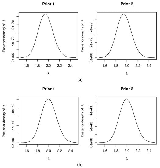
Figure 3. Posterior density plots of $\lambda$ for ${\eta }_1$ (a) with C.S ($S_3$, $T_6$), (b) with C.S ($S_2$, $T_5$).

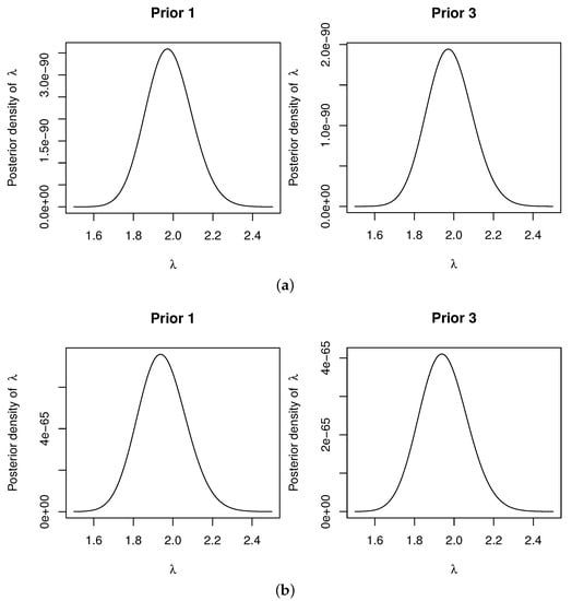
Figure 4. Posterior density plots of $\lambda$ for ${\eta }_2$ (a) with C.S ($S_3$, $T_6$), (b) with C.S ($S_2$, $T_5$).

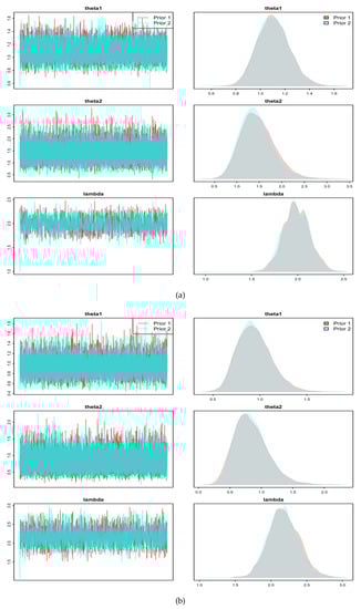
Figure 5. Trace plots for ${\eta }_1$ (a) with C.S ($S_2$, $T_5$), (b) with C.S ($S_4$, $T_1$).

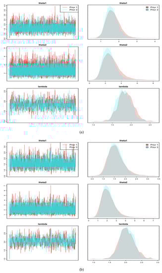
Figure 6. Trace plots for ${\eta }_2$ (a) with C.S ($S_3$, $T_3$), (b) with C.S ($S_4$, $T_4$).

To better compare the effects of the different estimates, in Table 2, Table 3, Table 4 and Table 5, we present the simulation results shown in Figure 7 for the point estimates and Figure 8 for the interval estimates. Note that the x-axis sequentially represents 12 different combinations of censoring schemes.

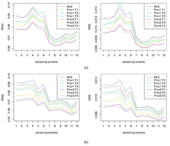
Figure 7. Visualization results of MADs and MSEs (a) for ${\eta }_1$, (b) for ${\eta }_2$.

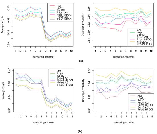
Figure 8. Visualization results of average lengths and coverage probabilities (a) for ${\eta }_1$, (b) for ${\eta }_2$.

In Figure 7, it can be seen that the Bayes estimates performed better in the majority of cases because they had lower MADs and MSEs. However, the Bayes estimate with non-informative priors, where F2 was chosen as the loss function, performed slightly worse. In the Bayes estimate, the informative priors had lower MADs and MSEs than the non-informative priors. In all cases, among the three loss functions, F3 performed the best, followed by F1, and F2 performed the worst. In addition, the performances of the different censoring schemes varied. For ${\eta }_1$, the censoring scheme ($S_2$, $T_5$) exhibited the smallest MADs and MSEs, and the censoring scheme ($S_3$, $T_6$) was the second-best performer. For ${\eta }_2$, the censoring scheme ($S_5$, $T_5$) exhibited the smallest MADs and MSEs, and the censoring scheme ($S_6$, $T_6$) was the second-best performer.

In Figure 8, it can be seen that BCIs and HPDCIs for the gamma informative priors performed the best, as they had the shortest average lengths and highest coverage probabilities. The logit-scale-based ACIs performed the second best. The ACIs and BootCIs performed the worst, as they had the longest average lengths and the lowest coverage probabilities. In all of these cases, in terms of the BCIs and HPDCIs, the HPDCIs had shorter average lengths, whereas the BCIs had higher coverage probabilities so they each have their own advantages. In addition, the informative priors outperformed the non-informative priors, as they exhibited both shorter average lengths and higher coverage probabilities. Furthermore, different censoring schemes also performed differently. For ${\eta }_1$, in terms of average lengths, the censoring scheme that performed the best was ($S_2$, $T_5$), whereas in terms of coverage probabilities, the censoring scheme that performed the best was ($S_4$, $T_4$). For ${\eta }_2$, in terms of average lengths, the censoring scheme that performed the best was ($S_5$, $T_5$), whereas in terms of coverage probabilities, the censoring scheme that performed the best was ($S_2$, $T_5$).

5.2. Real Data Example

To illustrate the suitability of the proposed method, a real data set was used. The data set we selected was obtained from http://cdec.water.ca.gov/cgi-progs/queryMonthly?SHA (accessed on 10 March 2023) and represents the water capacity of the Shasta reservoir in California, USA. We assumed that the water levels do not lead to excessive dryness if the reservoir capacities in August for at least 2 out of the next 5 years are not lower than the capacity observed in December of that year. Our purpose was to infer whether the area was excessively dry. Therefore, we can build a model to estimate the MSSR, where the capacities in August can be regarded as the strength variables and the capacity in December can be regarded as the stress variable. From 1975 to 2016, the water capacities in August and December were as follows:

$$X=\left(\begin{array}{ccccc}\hfill 0.287785\hfill & \hfill 0.126977\hfill & \hfill 0.768563\hfill & \hfill 0.703119\hfill & \hfill 0.729986\hfill \\ \hfill 0.811159\hfill & \hfill 0.829569\hfill & \hfill 0.726164\hfill & \hfill 0.423813\hfill & \hfill 0.715158\hfill \\ \hfill 0.363359\hfill & \hfill 0.463726\hfill & \hfill 0.371904\hfill & \hfill 0.291172\hfill & \hfill 0.414087\hfill \\ \hfill 0.538082\hfill & \hfill 0.744881\hfill & \hfill 0.722613\hfill & \hfill 0.561238\hfill & \hfill 0.813964\hfill \\ \hfill 0.668612\hfill & \hfill 0.524947\hfill & \hfill 0.605979\hfill & \hfill 0.715850\hfill & \hfill 0.529518\hfill \\ \hfill 0.742025\hfill & \hfill 0.468782\hfill & \hfill 0.345075\hfill & \hfill 0.425334\hfill & \hfill 0.767070\hfill \\ \hfill 0.613911\hfill & \hfill 0.461618\hfill & \hfill 0.294834\hfill & \hfill 0.392917\hfill & \hfill 0.688100\hfill \end{array}\right),\hspace{1em}Y=\left(\begin{array}{c}\hfill 0.667157\hfill \\ \hfill 0.767135\hfill \\ \hfill 0.640395\hfill \\ \hfill 0.650691\hfill \\ \hfill 0.709025\hfill \\ \hfill 0.824860\hfill \\ \hfill 0.679829\hfill \end{array}\right)$$

Before proceeding with the estimation, we first performed Kolmogorov–Smirnov (K-S) tests to ensure that X and Y did follow the Chen distribution. In addition, three distributions were used to compare with the Chen distribution in the K–S tests. Their PDFs are as follows:

$$\begin{array}{cc}\hfill \mathrm{Weibull}:& f(x)=\frac{\theta }{\lambda }{\left(\frac{x}{\lambda }\right)}^{\theta -1}{e}^{-{(\frac{x}{\lambda })}^{\theta }},x>0,\theta ,\lambda >0,\hfill \\ \hfill \mathrm{Burr}\mathrm{XII}:& f(x)=\theta \lambda x^{\theta -1}{(1+x^{\theta })}^{-\lambda -1},x>0,\theta ,\lambda >0,\hfill \\ \hfill \mathrm{Generalized}\mathrm{Rayleigh}:& f(x)=2\theta {\lambda }^{2}x{e}^{-{(\lambda x)}^2}{(1-e^{-{(\lambda x)}^2})}^{\theta -1},x>0,\theta ,\lambda >0.\hfill \end{array}$$

The results of the K–S tests are shown in Table 6. It can be seen that both X and Y followed the Chen distribution at the 0.05 significance level. In particular, the Chen distribution demonstrated better performance in the K–S tests for data set X.

Table 6. Comparison of different distributions in K–S tests.

Data Set	Distribution	$\widehat{\mathit{\theta }}$	$\widehat{\mathit{\lambda }}$	K–S Distance	p-Value
X	Chen	4.5946	3.5431	0.1461	0.4050
	Weibull	3.5428	0.6249	0.1550	0.3344
	Burr XII	3.7702	6.5519	0.1612	0.2908
	Generalized Rayleigh	2.2869	2.1350	0.1552	0.3329
Y	Chen	2.9026	3.6574	0.2337	0.7630
	Weibull	11.0177	0.7358	0.2297	0.7807
	Burr XII	11.1770	31.7219	0.2272	0.7913
	Generalized Rayleigh	1481.5031	3.9797	0.1966	0.9048

In the previous sections, the estimations of $R_{s,k}$ were discussed under the assumption that the stress and strength variables followed the Chen distribution with the same second shape parameter. Therefore, before estimating using the real data, we needed to check whether their second shape parameters were the same. Let $X_1,X_2,...,X_k$ follow $Chen({\theta }_1,{\lambda }_1)$ independently, and let Y (independent of $X_1,X_2,...,X_k$) follow $Chen({\theta }_2,{\lambda }_2)$. Then, the following hypothesis testing question is posed as

$$H_0:{\lambda }_1={\lambda }_2\hspace{1em}\mathrm{versus}\hspace{1em}{H}_1:{\lambda }_1\ne {\lambda }_2.$$

In the complete sample, the corresponding likelihood function is given by

$$\begin{array}{cc}\hfill L({\theta }_1,{\lambda }_1,{\theta }_2,{\lambda }_2)=& \prod _{i=1}^n\left(\prod _{j=1}^k{f}_X(x_{ij})\right)f_Y(y_i)\hfill \\ \hfill =& {{\theta }_1}^{nk}{{\lambda }_1}^{nk}{{\theta }_2}^n{{\lambda }_2}^n\prod _{i=1}^n\prod _{j=1}^k{x_{ij}}^{{\lambda }_1-1}\exp \{{x_{ij}}^{{\lambda }_1}+{\theta }_1(1-e^{{x_{ij}}^{{\lambda }_1}})\}\hfill \\ \hfill & \times \prod _{i=1}^n{y_i}^{{\lambda }_2-1}\exp \{{y_i}^{{\lambda }_2}+{\theta }_2(1-e^{{y_i}^{{\lambda }_2}})\}.\hfill \end{array}$$

Then, the likelihood ratio statistic is constructed as follows:

$$r=\frac{\underset{{\theta }_1,{\theta }_2>0,{\lambda }_1={\lambda }_2>0}{max}L({\theta }_1,{\lambda }_1,{\theta }_2,{\lambda }_2)}{\underset{{\theta }_1,{\theta }_2,{\lambda }_1,{\lambda }_2>0}{max}L({\theta }_1,{\lambda }_1,{\theta }_2,{\lambda }_2)}.$$

For large n, when $H_0$ holds, one has $\mathsf{\Lambda }=-2lnr\sim {\chi }^2(1)$ asymptotically. Thus, the rejection region is $\{\mathsf{\Lambda }>{\chi }_{\alpha }^2(1)\}$ at a given significance level $\alpha$, where ${\chi }_{\alpha }^2(1)$ is $100(1-\alpha )th$ percentile of ${\chi }^2(1)$. For given data sets X and Y, we calculate that $\mathsf{\Lambda }=0.2580$ with a p-value of 0.6115. Therefore, we can accept $H_0$ at the 0.05 significance level, whereupon the MSSR can be estimated using our proposed method.

Then, we obtain different estimates of $R_{s,k}$ using the complete sample, as well as three different censored samples. The samples can be, respectively, generated by the censoring schemes as follows:

$$\begin{array}{cc}\hfill & \mathrm{Complete}\mathrm{Sample}:S=(0*5),T=(0*7)(n=7,k=5,s=2).\hfill \\ \hfill & \mathrm{C}.\mathrm{S}1:S=(0,0,0,1),T=(0,0,0,1,1)(n=5,k=4,s=2).\hfill \\ \hfill & \mathrm{C}.\mathrm{S}2:S=(1,0,0,0),T=(2,0,0,0,0)(n=5,k=4,s=2).\hfill \\ \hfill & \mathrm{C}.\mathrm{S}3:S=(1,1,0),T=(1,1,1,0)(n=4,k=3,s=1).\hfill \end{array}$$

Based on C.S 1, the censored samples are derived as

$$X_1=\left(\begin{array}{cccc}\hfill 0.291172\hfill & \hfill 0.363359\hfill & \hfill 0.371904\hfill & \hfill 0.414087\hfill \\ \hfill 0.538082\hfill & \hfill 0.561238\hfill & \hfill 0.722613\hfill & \hfill 0.744881\hfill \\ \hfill 0.126977\hfill & \hfill 0.287785\hfill & \hfill 0.703119\hfill & \hfill 0.729986\hfill \\ \hfill 0.294834\hfill & \hfill 0.392917\hfill & \hfill 0.461618\hfill & \hfill 0.613911\hfill \\ \hfill 0.423813\hfill & \hfill 0.715158\hfill & \hfill 0.726164\hfill & \hfill 0.811159\hfill \end{array}\right),\hspace{1em}{Y}_1=\left(\begin{array}{c}\hfill 0.640395\hfill \\ \hfill 0.650691\hfill \\ \hfill 0.667157\hfill \\ \hfill 0.679829\hfill \\ \hfill 0.767135\hfill \end{array}\right)$$

Based on C.S 2, the censored samples are derived as

$$X_2=\left(\begin{array}{cccc}\hfill 0.291172\hfill & \hfill 0.371904\hfill & \hfill 0.414087\hfill & \hfill 0.463726\hfill \\ \hfill 0.294834\hfill & \hfill 0.461618\hfill & \hfill 0.613911\hfill & \hfill 0.688100\hfill \\ \hfill 0.524947\hfill & \hfill 0.605979\hfill & \hfill 0.668612\hfill & \hfill 0.715850\hfill \\ \hfill 0.423813\hfill & \hfill 0.726164\hfill & \hfill 0.811159\hfill & \hfill 0.829569\hfill \\ \hfill 0.345075\hfill & \hfill 0.468782\hfill & \hfill 0.742025\hfill & \hfill 0.767070\hfill \end{array}\right),\hspace{1em}{Y}_2=\left(\begin{array}{c}\hfill 0.640395\hfill \\ \hfill 0.679829\hfill \\ \hfill 0.709025\hfill \\ \hfill 0.767135\hfill \\ \hfill 0.824860\hfill \end{array}\right)$$

Based on C.S 3, the censored samples are derived as

$$X_3=\left(\begin{array}{ccc}\hfill 0.291172\hfill & \hfill 0.371904\hfill & \hfill 0.463726\hfill \\ \hfill 0.126977\hfill & \hfill 0.703119\hfill & \hfill 0.768563\hfill \\ \hfill 0.524947\hfill & \hfill 0.605979\hfill & \hfill 0.715850\hfill \\ \hfill 0.345075\hfill & \hfill 0.468782\hfill & \hfill 0.767070\hfill \end{array}\right),\hspace{1em}{Y}_3=\left(\begin{array}{c}\hfill 0.640395\hfill \\ \hfill 0.667157\hfill \\ \hfill 0.709025\hfill \\ \hfill 0.824860\hfill \end{array}\right)$$

For the complete, as well as three progressively censored, samples, we derive various point estimates and 95% interval estimates of $R_{s,k}$, as shown in Table 7 and Table 8, respectively. For the Bayesian estimates, non-informative priors are used. For three parameters in the MCMC method, we provide the CUSUM plots in Figure 9 and the trace plots in Figure 10. As can be seen in these figures, the MCMC chains converged quickly to stationary distributions, indicating that the MCMC method performed well.

Table 7. The point estimates for real data.

		Bayes
C.S	MLE	F1	F2	F3
Complete Sample	0.5133	0.5007	0.4632	0.5165
C.S 1	0.4339	0.4252	0.3724	0.4466
C.S 2	0.3630	0.3589	0.3075	0.3808
C.S 3	0.4858	0.4760	0.4044	0.5028

Table 8. The interval estimates for real data.

Intervals	Complete Sample	C.S 1	C.S 2	C.S 3
ACI	(0.2550, 0.7715)	(0.1480, 0.7199)	(0.1026, 0.6235)	(0.1421, 0.8294)
Logit	(0.2727, 0.7478)	(0.1931, 0.7106)	(0.1560, 0.6374)	(0.1927, 0.7890)
BootCI	(0.2860, 0.8142)	(0.1798, 0.8088)	(0.1500, 0.7633)	(0.1486, 0.8643)
BCI	(0.2555, 0.7463)	(0.1712, 0.7035)	(0.1394, 0.6273)	(0.1708, 0.7949)
HPDCI	(0.2531, 0.7411)	(0.1531, 0.6821)	(0.1267, 0.6108)	(0.1658, 0.7884)

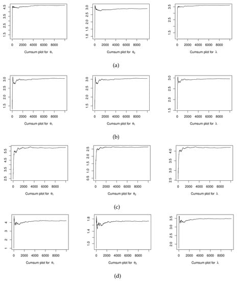
Figure 9. CUSUM plots for ${\theta }_1$, ${\theta }_2$, and $\lambda$ (a) with the complete sample, (b) with censoring scheme 1, (c) with censoring scheme 2, (d) with censoring scheme 3.

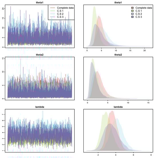
Figure 10. Trace plots for real data.

6. Conclusions

We study the estimation of the MSSR based on the Chen distribution using progressively censored data. The reliability inference of multicomponent stress–strength systems has attracted significant interest, with numerous scholars contributing to the field. Progressive Type-II censoring has been widely used in lifetime tests for nearly two decades. The Chen distribution is commonly used to model real-life data in the fields of lifetime analysis and reliability theory.

We begin by obtaining the MLE. Then, the ACI based on the MLE is derived, where the delta method is used. The percentile BootCI is also constructed. Additionally, the Bayes estimates, BCIs, and HPDCIs are obtained using the MCMC method. The stochastic simulations are performed using the R software. According to the results, the Bayes estimates under the gamma priors using the precautionary loss function exhibit the smallest MADs and MSEs among all the point estimates. Among all the interval estimates, the BCIs have the shortest lengths and the HPDCIs have the highest coverage probabilities. Finally, the applicability of the method is illustrated using real data.

Our study focuses solely on the estimation of the MSSR based on the Chen distribution using a common second shape parameter. In the future, we will explore the case of unequal shape parameters. Additionally, the multicomponent stress–strength system we study contains only one stress component and we do not consider scenarios involving multiple stress components. In the future, we will explore a more complex system and further extend the model to cases where there is more than one stress component. Furthermore, we assume that the strength random variables are independently and identically distributed, which may not accurately reflect certain real-world situations. Therefore, the study of multicomponent stress–strength systems with non-identical strength variables will be considered in the future.

References

- Weerahandi, S.; Johnson, R.A. Testing reliability in a stress-strength model when X and Y are normally distributed. Technometrics 1992, 34, 83–91. [Google Scholar] [CrossRef]
- Badr, M.M.; Shawky, A.I.; Alharby, A.H. The estimation of reliability from stress-strength for exponentiated Frechet distribution. Iran. J. Sci. Technol. Trans. A Sci. 2019, 43, 863–874. [Google Scholar] [CrossRef]
- Xu, H.; Yu, P.L.H.; Alvo, M. Detecting change points in the stress-strength reliability P(X<Y). Appl. Stoch. Model. Bus. Ind. 2019, 35, 837–857. [Google Scholar]
- Hassan, A.S.; Almanjahie, I.M.; Al-Omari, A.I.; Alzoubi, L.; Nagy, H.F. Stress-Strength Modeling Using Median-Ranked Set Sampling: Estimation, Simulation, and Application. Mathematics 2023, 11, 318. [Google Scholar] [CrossRef]
- Rao, G.S. Estimation of reliability in multicomponent stress-strength based on generalized exponential distribution. Rev. Colomb. Estad. 2012, 35, 67–76. [Google Scholar]
- Jia, J.M.; Yan, Z.Z.; Song, H.H.; Chen, Y. Reliability estimation in multicomponent stress-strength model for generalized inverted exponential distribution. Soft Comput. 2023, 27, 903–916. [Google Scholar] [CrossRef]
- Nadar, M.; Kizilaslan, F. Estimation of reliability in a multicomponent stress-strength model based on a Marshall-Olkin bivariate Weibull distribution. IEEE Trans. Reliab. 2016, 65, 370–380. [Google Scholar] [CrossRef]
- Kizilaslan, F.; Nadar, M. Estimation of reliability in a multicomponent stress-strength model based on a bivariate Kumaraswamy distribution. Stat. Pap. 2018, 59, 307–340. [Google Scholar] [CrossRef]
- Saini, S.; Tomer, S.; Garg, R. On the reliability estimation of multicomponent stress-strength model for Burr XII distribution using progressively first-failure censored samples. J. Stat. Comput. Simul. 2022, 92, 667–704. [Google Scholar] [CrossRef]
- Tsai, T.R.; Lio, Y.; Chiang, J.Y.; Chang, Y.W. Stress-Strength inference on the multicomponent model based on generalized exponential distributions under Type-I hybrid censoring. Mathematics 2023, 11, 1249. [Google Scholar] [CrossRef]
- Saini, S.; Tomer, S.; Garg, R. Inference of multicomponent stress-strength reliability following Topp-Leone distribution using progressively censored data. J. Appl. Stat. 2023, 50, 1538–1567. [Google Scholar] [CrossRef] [PubMed]
- Chen, Z.M. A new two-parameter lifetime distribution with bathtub shape or increasing failure rate function. Stat. Probab. Lett. 2000, 49, 155–161. [Google Scholar] [CrossRef]
- Chen, S.Y.; Gui, W.H. Statistical analysis of a lifetime distribution with a bathtub-shaped failure rate function under adaptive progressive Type-II censoring. Mathematics 2020, 8, 670. [Google Scholar] [CrossRef]
- Rastogi, M.K.; Tripathi, Y.M.; Wu, S.J. Estimating the parameters of a bathtub-shaped distribution under progressive type-II censoring. J. Appl. Stat. 2012, 39, 2389–2411. [Google Scholar] [CrossRef]
- Sarhan, A.M.; Hamilton, D.C.; Smith, B. Parameter estimation for a two-parameter bathtub-shaped lifetime distribution. Appl. Math. Model. 2012, 36, 5380–5392. [Google Scholar] [CrossRef]
- Mendez-Gonzalez, L.C.; Rodriguez-Picon, L.A.; Perez-Olguin, I.J.C.; Portilla, L.R.V. An Additive Chen Distribution with Applications to Lifetime Data. Axioms 2023, 12, 118. [Google Scholar] [CrossRef]
- Wang, L.; Wu, K.; Tripathi, Y.M.; Lodhi, C. Reliability analysis of multicomponent stress-strength reliability from a bathtub-shaped distribution. J. Appl. Stat. 2022, 49, 122–142. [Google Scholar] [CrossRef] [PubMed]
- Xu, J.; Long, J.S. Using the delta method to construct confidence intervals for predicted probabilities, rates, and discrete changes. Stata J. 2005, 5, 537–559. [Google Scholar] [CrossRef]
- Krishnamoorthy, K.; Lin, Y. Confidence limits for stress–strength reliability involving Weibull models. J. Stat. Plan. Inference 2010, 140, 1754–1764. [Google Scholar] [CrossRef]
- Stine, R. An introduction to bootstrap methods: Examples and ideas. Sociol. Methods Res. 1989, 18, 243–291. [Google Scholar] [CrossRef]
- Calabria, R.; Pulcini, G. Point estimation under asymmetric loss functions for left-truncated exponential samples. Commun. Stat. Theory Methods 1996, 25, 585–600. [Google Scholar] [CrossRef]
- Balakrishnan, N.; Sandhu, R.A. A simple simulational algorithm for generating progressive Type-II censored samples. Am. Stat. 1995, 49, 229–230. [Google Scholar]
Disclaimer/Publisher’s Note: The statements, opinions and data contained in all publications are solely those of the individual author(s) and contributor(s) and not of MDPI and/or the editor(s). MDPI and/or the editor(s) disclaim responsibility for any injury to people or property resulting from any ideas, methods, instructions or products referred to in the content. |
© 2023 by the authors. Licensee MDPI, Basel, Switzerland. This article is an open access article distributed under the terms and conditions of the Creative Commons Attribution (CC BY) license (https://creativecommons.org/licenses/by/4.0/).