Land–Air–Wall Cross-Domain Robot Based on Gecko Landing Bionic Behavior: System Design, Modeling, and Experiment

Abstract

Based on the bionic behavior of geckos, this paper presents a land–air–wall cross-domain robot which can fly in air, run on the ground, and adhere to various wall surfaces. When geckos jump and adsorb to vertical surfaces such as trunks, they can still adsorb to the wall with a large contact speed. Inspired by this phenomenon, we analyze the mechanism, apply it to our robot, and optimize the design of the robot structure. In addition, geckos use their tails to adjust posture to achieve abdominal landing during the process of falling. Inspired by this phenomenon, based on the rotor lift/power curve, we optimize the center of gravity by controlling the servo angle. The initial center of gravity offset of the robot is estimated by the extended state observer. The method reduces the distance between the center of gravity and the geometric center, balances the load of each propeller, and finally reduces the total power. The experiment and simulation results validate the feasibility of the land–air–wall cross-domain robot and the bionic methods.

1. Introduction

In recent years, land–air amphibious robots have become a hot research issue. Different countries have developed land–air amphibious robots with varied morphology. Land–air amphibious robots integrate the specialty of both flying robots and ground robots, including rapid space maneuverability and long-time working capability. At the same time, robots that are able to work in special environments have also attracted widespread attention. The flying adsorption amphibious robots have the ability to work in air and can perch on the surface of objects for a long time [1]. However, land–air amphibious robots cannot work on vertical surfaces for a long period of time, and the flying adsorption amphibious robots do not have ground motion capability.

1.1. Motivation

In order to combine the advantages of the land–air amphibious robot and the flying adsorption amphibious robot, this paper develops a land–air–wall cross-domain robot (LAWCDR) that can be widely used in disaster rescuing and battlefield reconnaissance environment monitoring.

By observing the behavior of geckos, the way they jump and attach to vertical surfaces caught our attention. When the front claws of the gecko come in contact with the vertical wall, the front claws are bounced off due to the excessive speed, and then the rear claws and tail remain attached to the wall. The geckos are able to adsorb to the surface with rear claws, tail, and spine. The mechanism of this phenomenon is applied to our robot (LAWCDR), in which two front wheels simulate the rear claws of geckos, and the suction cup and support bars simulate the head and front claws. After the wheels make contact with the wall, the suction cup (head) and support bars (front claws) are moved forward to make contact with the wall through the spine structure simulated by the servo to realize adsorption. The shock absorber of the wheels extends the dwelling time on the wall. Unlike real geckos, since our front wheels (rear claws) do not have a suction module, the front wheels may come off the wall after the suction cup (head) and support bars (front claws) come into contact with the wall.

In addition, the non-coincidence of the center of gravity and geometric center of the robot (LAWCDR) requires greater hovering power consumption. By observing the phenomenon that the belly landing is achieved by the gecko adjusting the attitude during the aerial motion, we adjust the body center of gravity in the air by adjusting the servos angle and reduce the aerial power by reducing the center of gravity offset.

1.2. Related Work

There are many different types of land–air amphibious robots. In 2009, the Hybird Land-Air Robot, researched by the University of Minnesota, folded the rotor of the vehicle in the ground state with the area between the two wheels, driven by ground motors. When flying, the robot stood up and unfolded to form a co-axial twin-rotor helicopter [2,3,4]. In 2013, the HyTAQ Robot was proposed by the Robotics Laboratory of the Illinois Institute of Technology. By installing an external roller cover that acts as a rotor shield and as a roller for ground motion, the ground part was powered by wind propulsion [5]. The robot called F-Star developed by Ben-Gurion University [6] had an adjustable angle of the arm while traveling on the ground, allowing F-Star to effectively raise or lower its fuselage when encountering an obstacle.

Flying adsorption amphibious robots can perch on the surface of objects in different ways, such as negative pressure adsorption [7,8], dry adsorption [9,10], and electrostatic adsorption. The collision of flying adsorption amphibious robots with walls and recovery from their collision have likewise received extensive attention. For example, Ref [11] used a compliant arm design that allowed it to fly freely while allowing a passive degree of freedom to absorb the impact. Additionally, Ref [12] installed a protective buffer around the rotor and modeled the collision of the airframe with a vertical wall. The simulation and experimental preliminary results verified the possibility and conditions for recovery from the collision. In [13], a collision recovery method was proposed for a quadrotor based on a protective cushion. It was validated by a comprehensive Monte Carlo collision bumper simulation, showing the feasibility of recovery from challenging collision scenarios. Research in [14] investigated the control problem of recovering a quadrotor after a collision with a rod object. In [15], the authors proposed a fast IMU-based collision detection method and potential field-based theory for collision recovery.

Designing flying adsorption amphibious robots through bionics is another effective method. Researchers have observed the existing roosting mechanisms in nature and applied them to robot design. For example, in [16,17,18] based on bat/gecko mimics, flight adsorption amphibious robots attached adsorption devices to multi-rotor vehicles for flight adsorption. In [19,20,21], the flight adsorption method based on bird claws was introduced. They used mechanical claws to mimic the claws of birds and made them capable of perching on various tree trunks. Furthermore, [22] used hooked claws and fixed-wing vehicles to achieve perching by mimicking the landing process of birds.

1.3. Contribution

In this paper, we mimic the behavior of the gecko and develop a land–air–wall cross-domain robot. The robot is capable of aerial flight, ground movement, and wall perching. Our robots have better adaptability compared to previous robots. For example, in disaster relief scenarios, the robot can maneuver quickly by flying, reconnoiter on the ground for a long time, or perch on the wall for surveillance and communication relay missions.

The specific contributions are as follows.

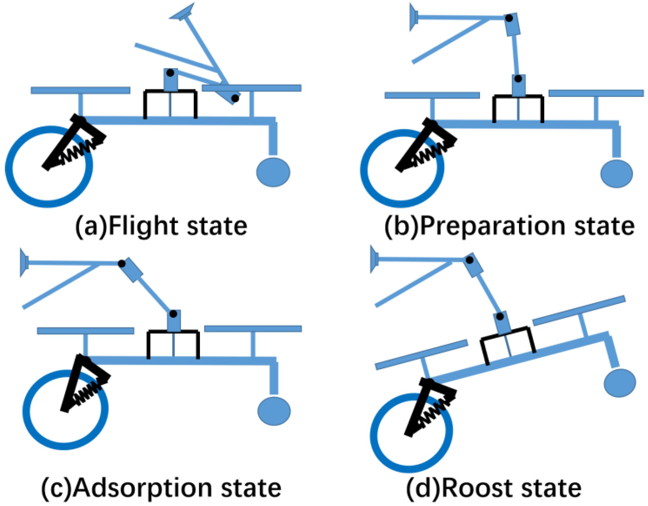
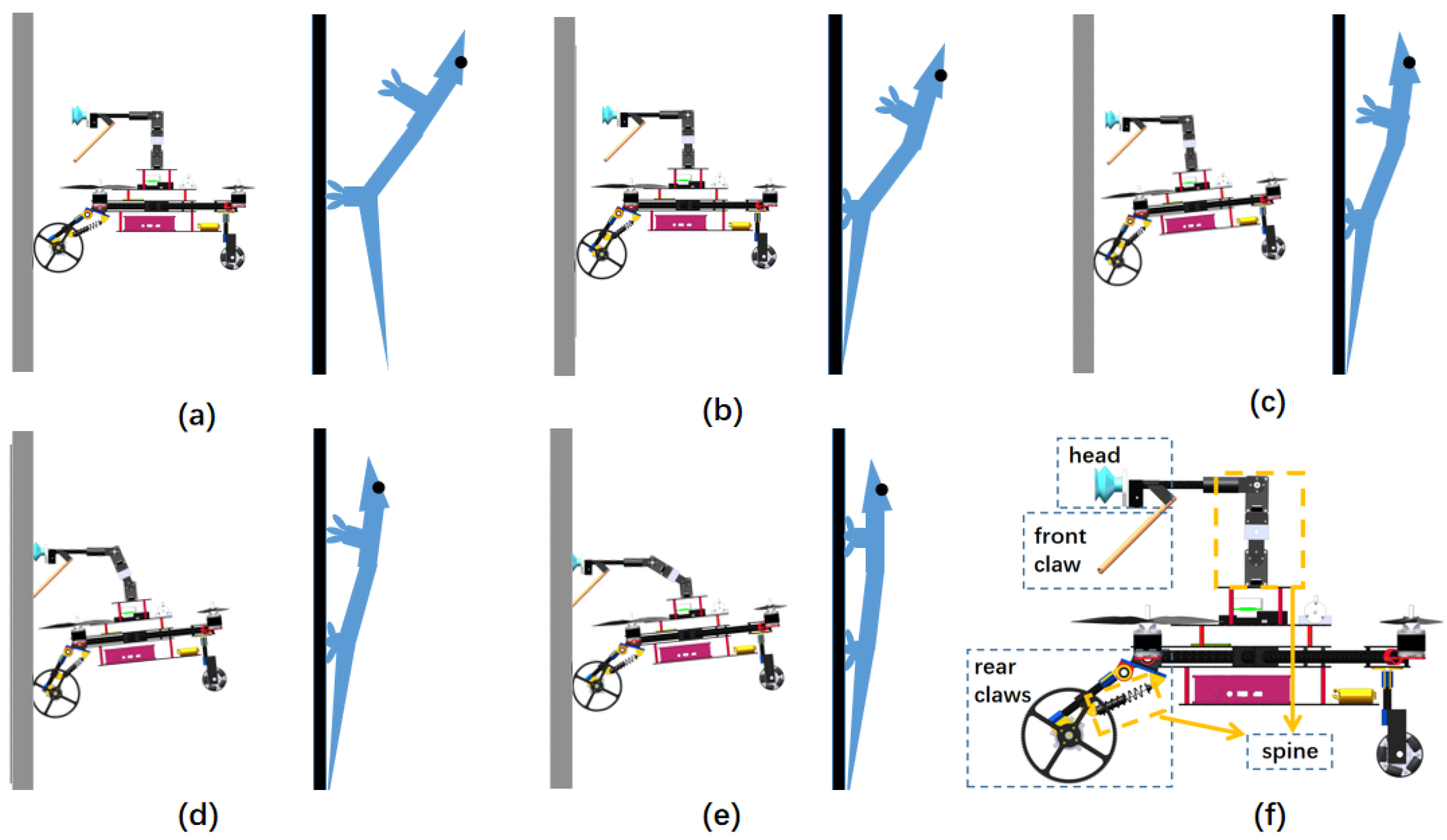
• By imitating the behavior of the gecko touching the wall, the robot can control the two joint movements for adsorption when the front wheels contact the wall. This mimics the gecko controlling the spine and tendons to achieve the process of adsorption. Compared with previous flying adsorption amphibious robots, our bionic adsorption method reduces the requirement for the position feedback so that it is more suitable for practical scenarios. This is achieved by giving a certain pitch angle to first make contact between the wheel and the wall, and then controlling the servos to perform the adsorption. Position or force feedback are not necessary for the perching process.
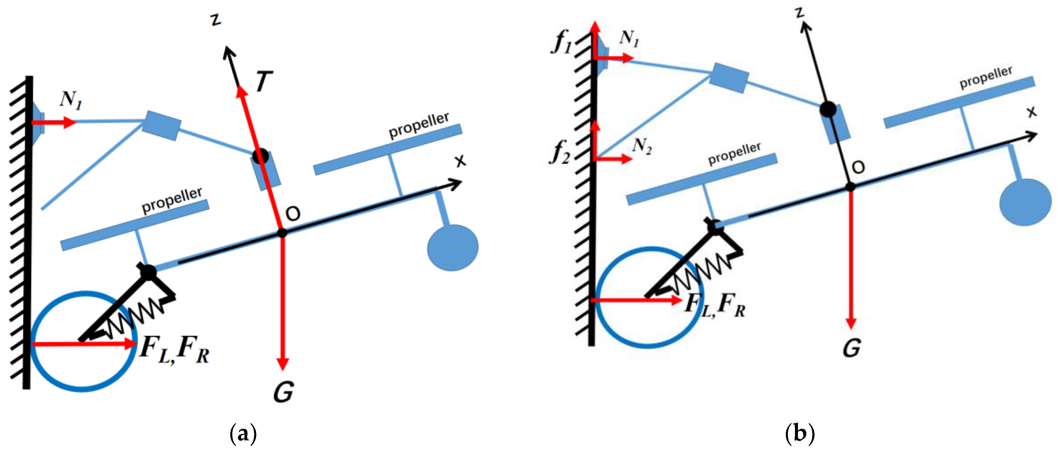
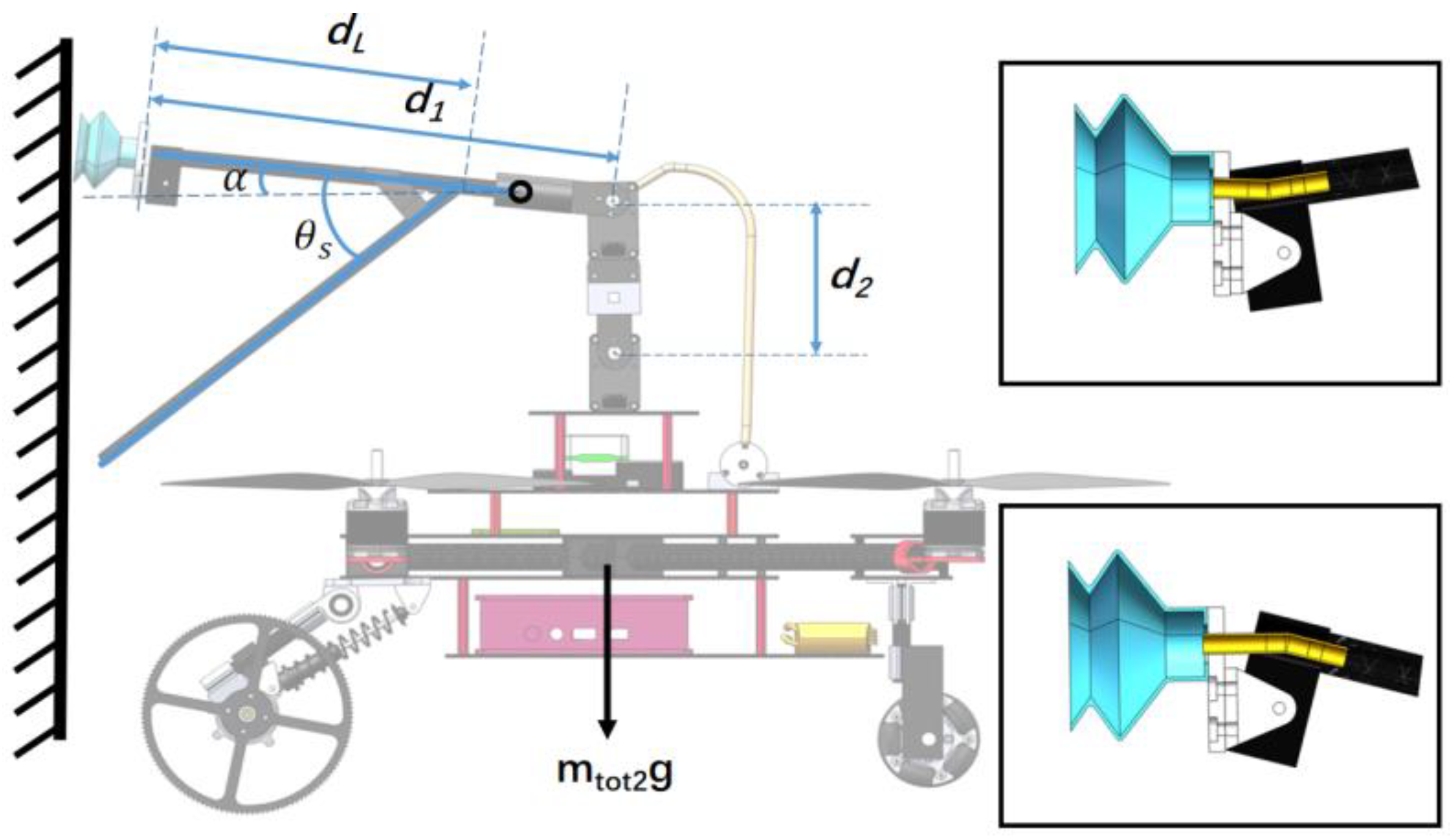
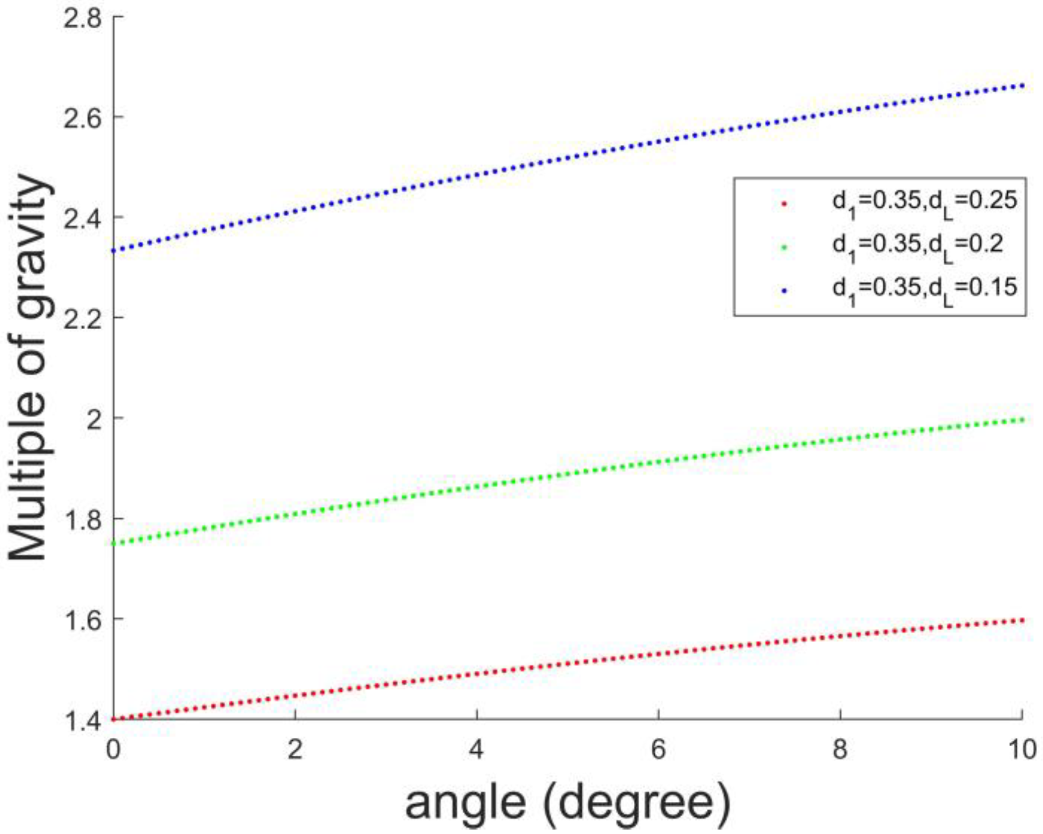
• We design the mechanical structure to protect the rotor from contact with the wall and crashing. The optimized design of the adsorption device is carried out through the force analysis of the robot during the adsorption process.
• We mimic the behavior of the gecko in regulating its attitude during landing. The initial center of gravity offset of the robot is observed by the extended state observer. Based on the lift/power curve, we balance the load of the four propellers by adjusting the joint angle to reduce the hovering power and improve the endurance.

1.4. Outline

This paper is organized as follows. In Section 2, we introduce the overall structural design and optimization of the land–air–wall cross-domain robot (LAWCDR). In Section 3, we present the dynamics modeling and control of the robot during different motions. Simulation and experimental results are given in Section 4 to verify the effectiveness of the robot (LAWCDR). The paper ends with conclusions in Section 5.

2. System Design and Optimization

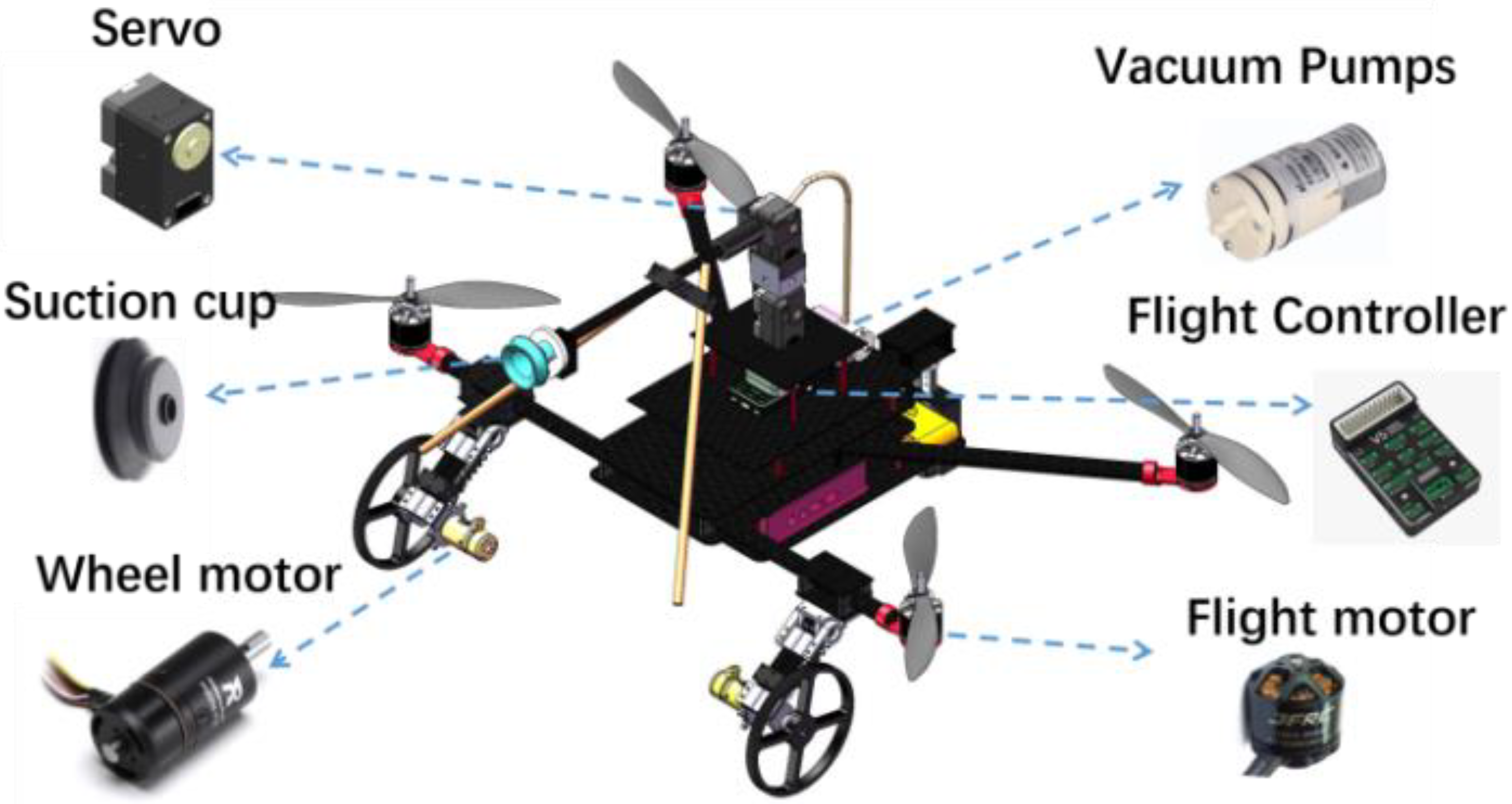
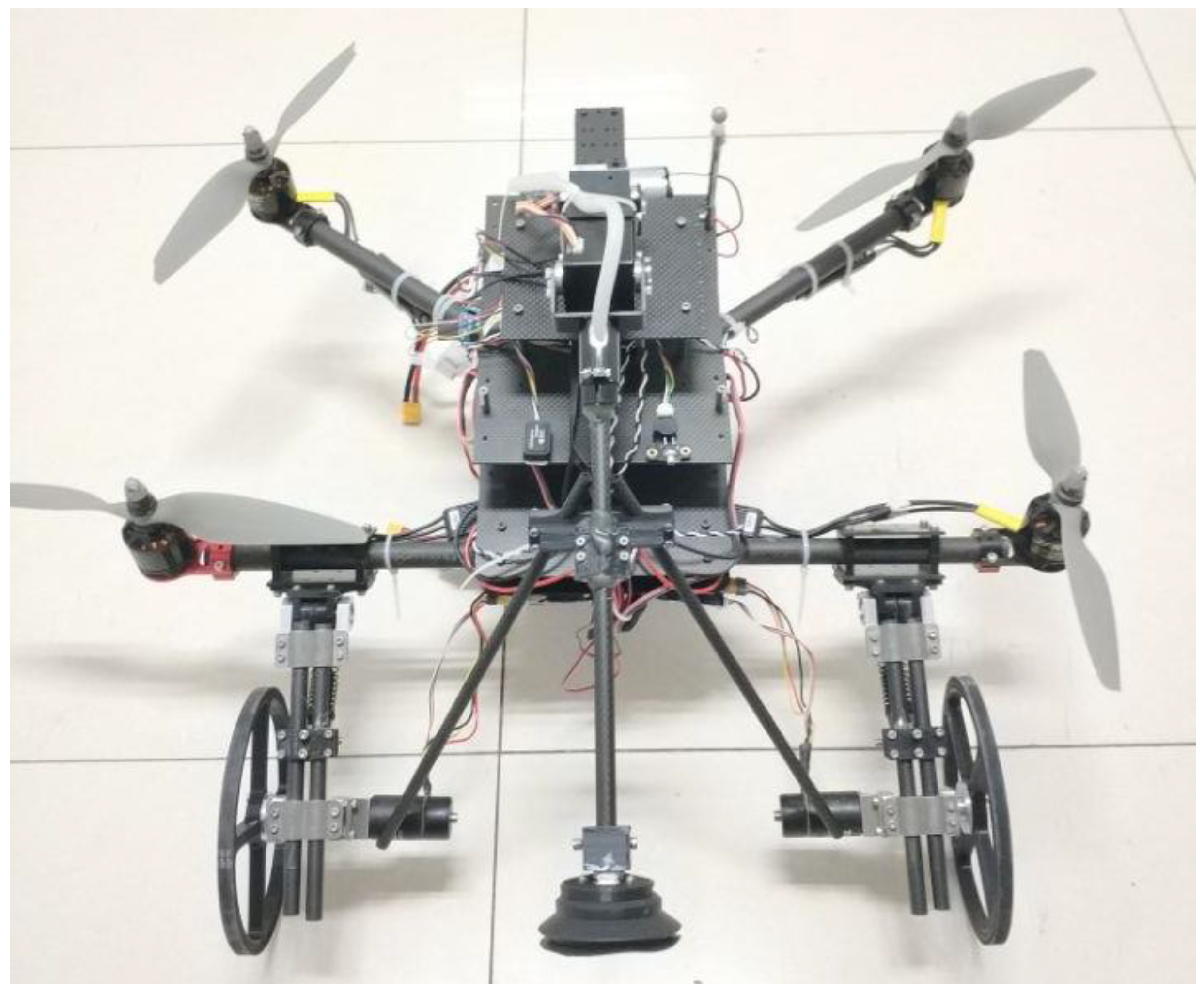
2.1. Overall Structural Design of Robot (LAWCDR)

The overall design of the land–air–wall cross-domain is shown in Figure 1, which mainly includes the ground module, the flight module, and the adsorption module. The ground module consists of the front wheels with shock absorbers and an omni-directional rear wheel. The robot turns by the differential speed of the two front wheels. The shock absorber is mainly responsible for providing a certain cushioning force and correcting heading when the robot contacts the wall during the adsorption process. The shock absorber does not work when it is on the ground, and the spring stretches to its maximum stroke under gravity.

The flight module mainly includes four rotor motors and the corresponding propellers, which are responsible for flying in three-dimensional space. The adsorption module consists of a suction cup, a vacuum pump, support bars, carbon tubes and silicone tubes connecting the various parts, and two RS485 servos responsible for the movement of the suction cup. While perching on the wall, the support bars prevent the suction cup from peeling off the wall due to the rotational torque generated by gravity. In addition, the wheel and the support bars work together to prevent the propellers from contacting the wall.

The structure and coordinates of the robot are shown in Figure 2, and the inertial coordinate system is represented by $O_w$, $O_b$, $O_h$, and $O_c$ respectively, where $O_w$ denotes the world coordinate system and $O_b$ denotes the body coordinate system. $T_i$ denotes the lift generated by the ith rotor. The angular bisector of the second and third motors is taken as the y-axis, and the angular bisector of the third and fourth motors is taken as the x-axis. $O_h$ and $O_c$ denote the coordinate systems represented by the first and second joints, and $O_c$ coincides with the suction cup end coordinate system. The x-axis distance from the rotor to the geometric center of the body is $l$, the distance from the first joint to the second joint is $d_2$, and the first joint is fixedly connected to the robot. The distance between the second joint and the suction cup is $d_1$. $h$ denotes the z-axis distance of $O_h$ of the body coordinate system.

As shown in Figure 3, the robot can generally be divided into four working states. (a) Flight state: when the servo is adjusted to the best position, the power consumption is reduced according to the mass distribution. (b) Preparation state: as a preparatory state for adsorption, the suction cup is adjusted to appropriate position to reduce the robot’s reaction time when the wheels are in contact with the wall. (c) Adsorption state: a single-line LIDAR is used to detect the relative position and attitude between the robot and the wall. The head and front claws of the robot are controlled to face the wall. After the robot detects its contact with the wall, the robot controls the servo to reach forward to achieve adsorption. (d) Roost state: at this time, the propellers and servos are stopped to save power and reduce heat. The robot adsorbs on the wall under the action of the vacuum pump and support bars. Because the body is in a free state, the front wheels are compressed, but they still prevent propellers from contacting the wall.

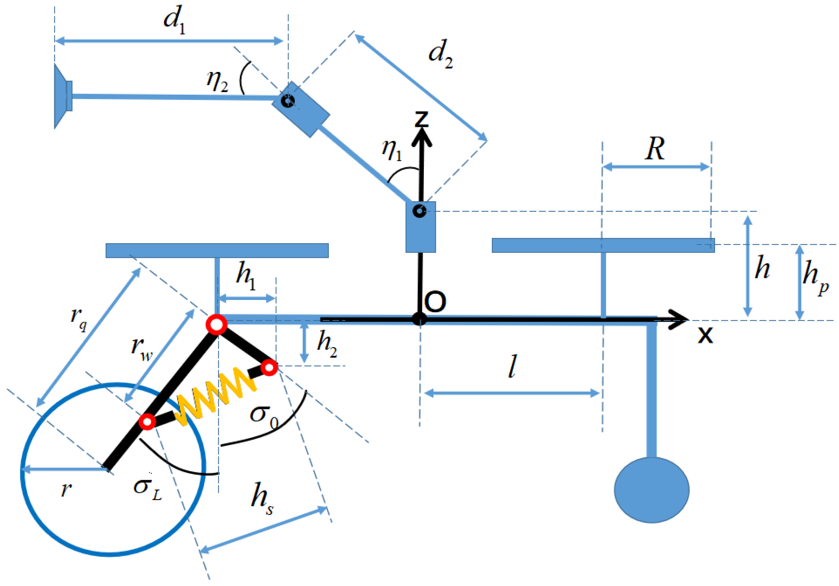
2.2. Design and Analysis of the Adsorption of Bionic Structures

The robot (LAWCDR) mainly mimics the process of a gecko perching on a vertical surface even after the collision, rather than being bounced off. In [23], Jusufi analyzed the slow motion of an Asian flat-tailed gecko (Hemidactylus platyurus) jumping from trunk to trunk, which allows the gecko to grasp the trunk through the sticky toe pads of its hind paws when it is bounced back from a vertical surface, with the tail providing leverage for the gecko to counteract the moment of flipping backward and again allowing the front paws to contact with the wall. The researchers designed a simulated gecko equipped with four Velcro feet and a tail to control the body flexion of the gecko through internal tendons. Experiments have shown that the simulated gecko with the tail was able to increase the adsorption success rate from 15% to 55%. In nature, the tail helps the gecko increase its landing success rate from nearly 0% to 87%.

We mimic the spine of a gecko by shock absorbers and a two servos mechanism. When the wheels come into contact with the wall, the moment causes the body to rotate and affects the forward reaching of the suction cup. The front claws keep stretching out in order to improve the success rate of the adsorption. The wheels (rear claws) stay on the wall and provide guidance of the heading before the front claw stretches out and makes contact with the wall. As shown in Figure 4, (a) the wheels (rear claws) start to contact the wall. (b) The wheels (rear claws) are compressed to produce a tilting moment. (c) The robot uses the lift force generated by the propeller to attach the wheels to the wall. (d) The suction cup (head) and support bars (front claws) are driven towards the wall by adjusting the posture with the servos (spine). (e) The suction cup is attached to the wall, establishes a negative pressure environment, and makes the robot adsorb to the wall. The rotor stops working. Panel (f) indicates the bionic function of each component.

The structural dimensions of the robot (LAWCDR) are shown in Figure 5. The model of the wheel–wall contact can be represented as

$$\{\begin{array}{l}{M}_{\theta }=F_L{d}_{wl}+F_R{d}_{wr}-l{k}_f{\omega }_1^2-l{k}_f{\omega }_2^2+l{k}_f{\omega }_3^2+l{k}_f{\omega }_4^2+M_G\\ M_{\psi }=F_L{l}_3-F_R{l}_3+k_m{\omega }_1^2-k_m{\omega }_2^2+k_m{\omega }_3^2-k_m{\omega }_4^2\end{array}$$

(1)

where $M_{\theta }$ and $M_{\psi }$ are the y-axis and z-axis moment. $M_G$ is the gravitational moment. $F_L$ and $F_R$ are the equivalent contact forces of the left and right wheel on the wall. $d_{wl}$ and $d_{wr}$ are the z-axis distances of the left and right wheel contact points with the wall in the body coordinate system, and $l_3$ is the y-axis distance from the two front wheels to the center of the body. ${\omega }_i$ is the rotational speed of the ith rotor. Take the left wheel as an example.

$$d_{wl}=r_q\cos ({\sigma }_L-\theta )+l\sin \theta$$

(2)

$$F_L{d}_{wl}-k_s•r_w\sin ({\sigma }_0+{\sigma }_L)\sqrt{h_1^2+h_2^2}=I_w{\ddot{\sigma }}_L$$

(3)

where $I_w$ is the rotational inertia of the wheel assembly. $k_s$ is the coefficient of elasticity of the spring. $r_w$ is the rotation radius of the spring assembly. $r_q$ is the rotation radius of the wheel assembly. $h_1$ and $h_2$ are the x-axis distance and z-axis distance of the spring mount point in the body coordinate system, respectively. ${\sigma }_L$ is the angle between the carbon tube of the wheel assembly and the z-axis in the body coordinate system. $h_p$ is the height of the propeller in the body coordinate system. $R$ is the radius of the propeller. $r$ is the radius of the wheel. The length of the spring, $h_s$, is represented in the following equation.

$$h_s=\sqrt{(r_w^2+h_1^2+h_2^2-2\cdot r_w\cdot \sqrt{(h_1^2+h_2^2)}cos({\sigma }_0+{\sigma }_L))}$$

(4)

$$tan({\sigma }_0)=\frac{h_1^{}}{h_2^{}}$$

(5)

It must be ensured that the propeller cannot exceed the plane formed by the two front wheels and the suction cup when the robot is in contact with the wall. The coordinate of the suction cup in the world coordinate system is expressed as follows:

$$p_{sc}=\left[\begin{array}{c}{x}_{sc}\\ y_{sc}\\ z_{sc}\end{array}\right]=\left[\begin{array}{c}{x}_b\\ y_b\\ z_b\end{array}\right]+R_b^w\left[\begin{array}{c}-d_{2}sin{\mathsf{\eta }}_1-d_{1}sin({\mathsf{\eta }}_1+{\mathsf{\eta }}_2)\\ 0\\ h+d_{2}cos{\mathsf{\eta }}_1+d_{1}cos({\mathsf{\eta }}_1+{\mathsf{\eta }}_2)\end{array}\right]$$

(6)

The coordinate of the contact point between the wheels and the wall is expressed as follows:

$$p_{wheel}=\left[\begin{array}{c}{x}_{wheel}\\ y_{wheel}\\ z_{wheel}\end{array}\right]=\left[\begin{array}{c}{x}_b\\ y_b\\ z_b\end{array}\right]+R_b^w\left[\begin{array}{c}-l-r_{q}sin{\sigma }_L\\ -l_3\\ -r_{q}cos{\sigma }_L\end{array}\right]+\left[\begin{array}{c}-rcos\psi \\ rsin\psi \\ 0\end{array}\right]$$

(7)

The coordinate of the point on the propeller closest to the wall is expressed as follows:

$$p_{prop}=\left[\begin{array}{c}{x}_{prop}\\ y_{prop}^{}\\ z_{prop}\end{array}\right]=\left[\begin{array}{c}{x}_b\\ y_b\\ z_b\end{array}\right]+R_b^w\left[\begin{array}{c}-(l+\mathrm{R})\\ \pm l\\ h_p\end{array}\right]$$

(8)

In order to protect the propeller, when the suction cup and the wheels are in contact with the wall, the propellers are prevented from obtaining contact with the wall. In order to simplify the model, when the wheel is at the maximum compression, $p_{prop}$ and $p_b$ are simultaneously on the same side of the line formed by the suction cup and the wheel.

In the x-z plane, the equation of the line passing through $p_{wheel}$ and $p_{prop}$ is shown in the following equation:

$$f(x,z)=[(z-z_{wheel})(x_{sc}-x_{wheel})-(x-x_{wheel})(z_{sc}-z_{wheel})]$$

(9)

Therefore,

$$f(x_{prop},z_{prop})•f(x_b,z_b)>0$$

(10)

The constraint of ${\mathsf{\eta }}_1$ and ${\mathsf{\eta }}_2$ can be calculated by Equations (6)–(8) and (10).

The force of the robot is shown in Figure 6a. If the wheel is in a free state, the friction between the wall and the front wheels belongs to rolling friction, which is much smaller than the sliding friction (ignoring the rolling friction). $f_1$ denotes the friction between the suction cup and the wall, and $f_2$ denotes the friction between the support bars and the wall. $N_1$ and $N_2$ are the support forces of the wall for the suction cup and the support bars, respectively. $T$ and $G$ denote the total lift and gravity force, respectively.

As shown in Figure 6b, after adsorption succeeds, the robot loses the lift force $T$ generated by the propeller. Therefore, we need the frictional forces $f_1$ and $f_2$ provided by the wall to balance with the gravity force $G$. At this time, the two servos can be in a free state to avoid the heat generated by the long working time.

In order to increase the weight capacity of the adsorption module, the structure of the suction cup and the support bars is shown in Figure 7. The angle between the carbon fiber tube which is connected to the suction cup and the support bars is ${\theta }_s$. The angle between the carbon fiber tube attached to the suction cup and the horizontal plane is $\alpha$. Ignoring the mass of the support bars and the carbon fiber tube, the forces in the horizontal and vertical directions are balanced.

$$\{\begin{array}{l}{N}_1+N_2=F_{suction}\\ f_1+f_2=mg\end{array}$$

(11)

Additionally,

$$\{\begin{array}{l}{f}_1\le {\mu }_1{N}_1\\ f_2\le {\mu }_2{N}_2\end{array}$$

(12)

$$(F-N_1)d_L[sin\alpha +\tan ({\theta }_s-\alpha )\cos \alpha ]=mg{d}_1\cos \alpha$$

(13)

where ${\mu }_1$ is the coefficient of friction between the suction cup and the wall, and ${\mu }_2$ is the coefficient of friction between the support bars and the wall. $d_L$ is the distance from the connection point of the support bars to the suction cup. $m$ is the mass of the robot and $g$ denotes the acceleration of gravity

$$N_2=\frac{mg{d}_1\cos \alpha }{d_L\sin \alpha +d_L\cos \alpha \tan ({\theta }_s-\alpha )}$$

(14)

Because suction cup and support bars are not the same material, ${\mu }_1$ and ${\mu }_2$ are not consistent. In general, ${\mu }_1<{\mu }_2$, therefore it is necessary to raise $N_2$ to increase the weight that the robot can hold.

The influence of $N_2$ on $\alpha$ is shown in Figure 8. $N_2$ becomes larger as $\alpha$ increases. As $\alpha$ becomes larger, the robot assigns more $F_{suction}$ to $N_2$. Assuming $d_1=0.35$ m,$d_L=0.2$ m, $N_2$ is approximately equal to $1.996\times mg$ when $\alpha =10°$ which is 1.14 times as large as $N_2=1.75\times mg$ when $\alpha =0°$. The increase of $\alpha$ may cause the suction cup to be unable to fit against the wall and form a negative pressure environment. Therefore, we increased the contact angle of the suction cup by adding a pivot and a limit block, as shown in Figure 7. The suction cup is connected to the robot by a pivot and is limited by a limit block. The suction cup and the carbon fiber tube are connected by a flexible silicone tube. Therefore, the suction cup can rotate $[-5°,5°]$ on the limit block, and because the double-layer suction cup itself has $[-6.75°,6.75°]$ angle range, the robot’s suction cup has $[-11.75°,11.75°]$ angle range.

As shown in Figure 9, we tested the variation of $N_2$ for different clamping angles of the support bars ${\theta }_s$. As the clamping angle ${\theta }_s$ becomes larger, $N_2$ gradually becomes smaller. However, $N_1$ cannot be lower than a certain threshold, otherwise it will lead to an increase in the leakage rate of the suction cup and further lead to the disengagement of the suction cup. Therefore, we take ${\theta }_s$ as 45 degrees. When the suction cup works on the surface of the painted wall, the pressure difference is 40 kpa, and the diameter suction cup is 0.03 m. $F_{suction}$ is about 110 N. The total mass of the robot is 3 kg. Then, the maximum friction force that the robot can provide is about 69.37 N, which is two times greater than the gravity.

3. Dynamic Model and Control

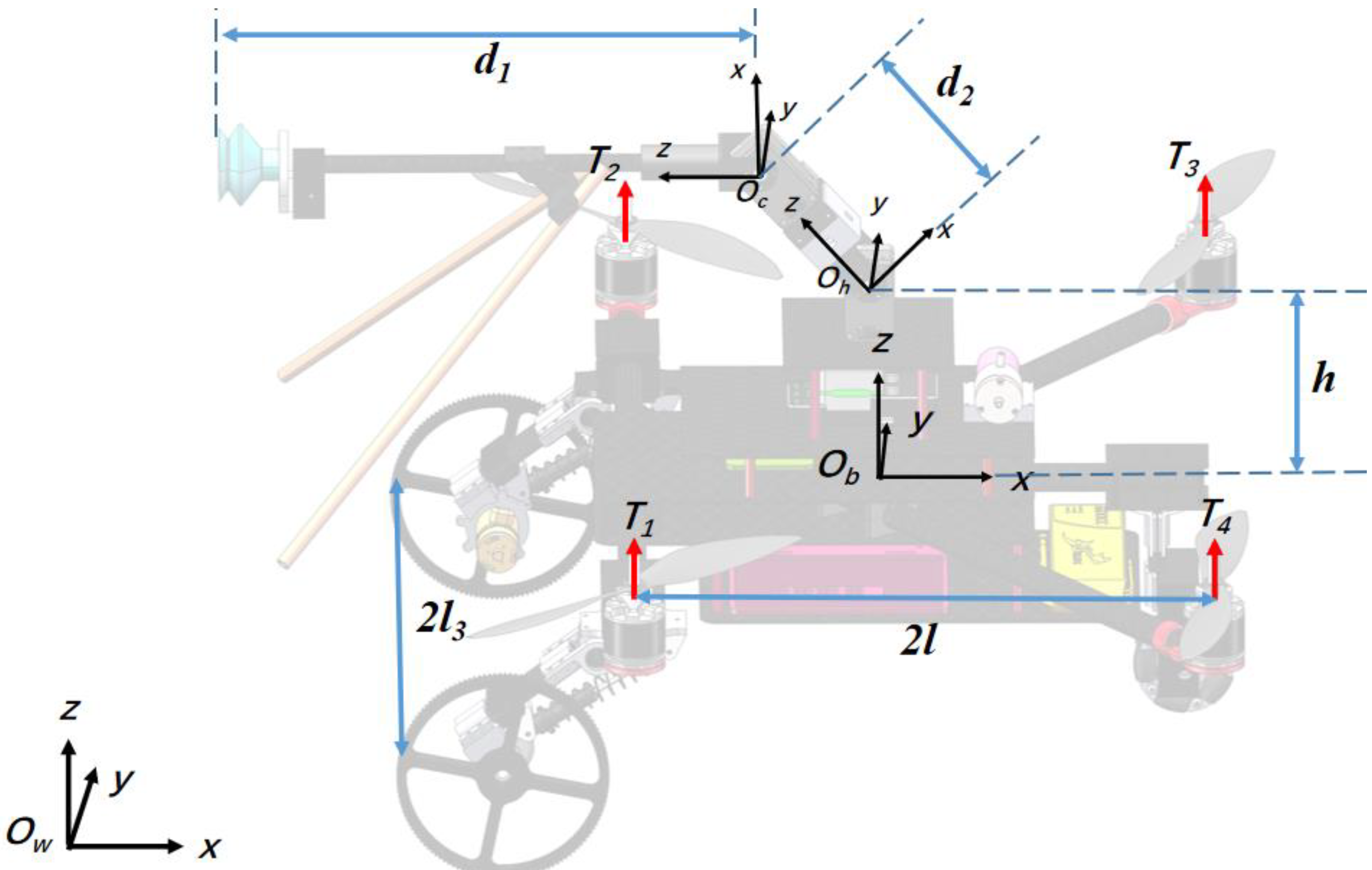
3.1. Air Dynamics Modeling and Ground Dynamics Modeling

The position of the robot in the world coordinate system is $p_w={(x,y,z)}^T$ and the attitude angle is $\Omega ={(\phi ,\theta ,\psi )}^T$. The joint angle of the two servos is $\eta ={({\mathsf{\eta }}_1,{\mathsf{\eta }}_2)}^T$. The rotation matrix $R_b^w$ between $O_w$ and $O_b$ is denoted as:

$$R_b^w=\left[\begin{array}{ccc}c\psi c\theta & c\psi s\theta s\phi -s\psi c\phi & c\psi s\theta c\phi +s\psi s\phi \\ s\psi c\theta & s\psi s\theta s\phi +c\psi c\phi & s\psi s\theta c\phi -c\psi s\phi \\ -s\theta & c\theta s\phi & c\theta c\phi \end{array}\right]$$

(15)

where $c\theta$ denotes $cos\left(\theta \right)$ and $s\theta$ denotes $sin\left(\theta \right)$. $c\phi$ denotes $cos\left(\phi \right)$ and $s\phi$ denotes $sin\left(\phi \right)$. $c\psi$ denotes $cos\left(\psi \right)$ and $s\psi$ denotes $sin\left(\psi \right)$.

$$\begin{array}{l}\varphi ,\theta \in (-\pi /4,\pi /4)\\ \psi \in (-\pi ,\pi ]\\ {\mathsf{\eta }}_1,{\mathsf{\eta }}_2\in [-\pi /2,\pi /2]\end{array}$$

The dynamics model of the robot can be represented using the Euler–Lagrange equations.

$$\mathrm{M}(q)\ddot{q}+C(q,\dot{q})\dot{q}+G(q)=B\tau$$

(16)

where $q={[p_w{}^T,{\Omega }^T,{\mathsf{\eta }}^T]}^T$ is the vector containing all the generalized coordinate variables. $M(q)$ is the inertia matrix, $C(q,\dot{q})$ is the Coriolis matrix, $G(q)$ is the gravity vector, $\tau$ is the generalized moment input, and $B$ is the input transformation matrix. The inertia matrix $M(q)$ is shown as follows [24]:

$$\mathrm{M}(q)=M_{t,b}^T{m}_b{M}_{t,b}^{}+M_{r,b}^{T}R{I}_b{R}^T{M}_{r,b}^{}+{\displaystyle \sum _{i=1}^2{M}_{t,i}^T{m}_i{M}_{t,i}^{}+M_{r,i}^T(R{R}_i)I_i{(R{R}_i)}^T{M}_{r,i}^{}}$$

(17)

where $M_{t,b}^{}=\frac{\dot{p}}{\dot{q}},M_{r,b}^{}=\frac{\omega }{\dot{q}},M_{t,i}^{}=\frac{{\dot{p}}_i}{\dot{q}},M_{r,i}^{}=\frac{{\omega }_i}{\dot{q}}$ are the matrices that form a velocity relationship. $\dot{p}$ and $\omega$ are the translational and angular velocity of body in the inertial frame. ${\dot{p}}_i$ and ${\omega }_i$ are the translational and angular velocity of ith joint in the inertial frame. $m_b$ and $m_i$ are the mass of the body and the ith joint. $I_b$ and $I_i$ are the rotational inertia of the body and the ith joint. $R=R_b^w$. $R_i$ denotes the rotation matrix from the body frame to the ith joint.

The Corillis matrix $C(q,\dot{q})$ is shown as follows [24,25]:

$$c_{kj}={\displaystyle \sum _{i=1}^8\frac{1}{2}}\{\frac{\partial m_{kj}}{\partial q_i}+\frac{\partial m_{ki}}{\partial q_j}-\frac{\partial m_{ij}}{\partial q_k}\}{\dot{q}}_i$$

(18)

where $c_{kj}$ indicates the element of $C(q,\dot{q})$ at the kth row and jth column. $m_{ab}$ indicates the element of $M(q)$ at the ath row and bth column.

The gravity vector $G(q)$ is shown as follows:

$$\{\begin{array}{l}G(q)=\frac{\partial U}{\partial q}\\ U=m_{b}g{e}_g^T{p}_w+{\displaystyle \sum _{i=1}^2{m}_{i}g{e}_g^T(p_w+R_i{p}_i^b)}\end{array}$$

(19)

where $e_g$ is the unit vector ${[\begin{array}{ccc}0& 0& 1\end{array}]}^T$. $p_i^b$ denotes the position of the ith joint in the body coordinate system. $U$ is the potential energy of the robot.

Although the Euler–Lagrange Equation (16) can describe the motion of the robot, the accumulated dynamic model is too complicated to design an efficient controller. Because the range of motion of the joints during adsorption is limited, the joint firstly needs to be adjusted to the preparation state and the mass of the joints is small compared to the rest of the robot. Thus, we decouple the joint and the robot body, use the motion at the end of the suction cup as a perturbation to the robot body, and improve the efficiency of the control.

The rotor lift is expressed by the following equation.

$$T_i=k_f{\omega }_i^2$$

(20)

$$T_{tot}={\displaystyle \sum _{i=1}^4{k}_f{\omega }_i^2}$$

(21)

where $T_i$ is the ith rotor lift, $k_f$ is the lift coefficient, ${\omega }_i$ is the rotational speed of the ith rotor. $T_{tot}$ is the total lift of the robot.

The dynamics model of robot is shown in the following equation, ignoring air resistance.

$$\{\begin{array}{l}(m+m_s+m_v){\ddot{p}}_w=R_b^w{T}_{tot}-(m+m_s+m_v)g+F_{\mathrm{ext}}\\ I\stackrel{•}{\omega }=-\omega \times I\omega +M\\ \mathsf{\eta }=A\end{array}$$

(22)

where $A=\left[\begin{array}{c}{\mathsf{\eta }}_{\theta }\\ -{\mathsf{\eta }}_{\theta }-\theta \end{array}\right]$ and $d_2\sin {\mathsf{\eta }}_{\theta }$ is the relative forward extension of the suction cup. $m$ is the mass of the body, $m_s$ is the mass of the first joint, and $m_v$ is the mass of second joint.

In the actual robot adsorption process, the roll angle is always close to 0 degrees in order to maintain the robot balance. Therefore, M can be expressed as follows.

$$M=\left[\begin{array}{ccccccc}-l{k}_f& l{k}_f& l{k}_f& -l{k}_f& 0& 0& 0\\ -l{k}_f& -l{k}_f& l{k}_f& l{k}_f& L_1& d_2\sin {\mathsf{\eta }}_1& d_2\sin {\mathsf{\eta }}_1+d_1\sin ({\mathsf{\eta }}_1+{\mathsf{\eta }}_2)\\ k_m& -k_m& k_m& -k_m& 0& 0& 0\end{array}\right]\left[\begin{array}{l}{\omega }_1^2\\ {\omega }_2^2\\ {\omega }_3^2\\ {\omega }_4^2\\ mg\\ m_{s}g\\ m_{v}g\end{array}\right]+\left[\begin{array}{l}0\\ {\tau }_{ext}\\ 0\end{array}\right]$$

(23)

where $k_m$ is the drag coefficient. ${\tau }_{ext}$ is the moment due to the external force $F_{ext}$. $L_1$ is the y-axis moment of the body mass in the body coordinate system.

When the suction cup is not in stable contact with the wall, the suction cup makes contact with the wall at small speeds modeled by a spring damping model.

$$F_{ext}=\left[\begin{array}{c}0\\ F_L+F_R+F_{sc}\\ 0\end{array}\right]$$

(24)

$$\{\begin{array}{l}{F}_{sc}=\{\begin{array}{l}K\left|\delta \right|+C\stackrel{•}{\delta },\delta <0\\ 0,\delta \ge 0\end{array}\\ \delta =x_p-d_2\sin {\mathsf{\eta }}_1-d_1\sin ({\mathsf{\eta }}_1+{\mathsf{\eta }}_2)\end{array}$$

(25)

where $x_p$ is the distance between $O_b$ and the wall, $K$ is the contact stiffness, and $C$ is the damping coefficient.

The velocity $v_0$ and angular velocity $w_0$ of the ground motion of the robot are shown in the following equation.

$$\{\begin{array}{l}{v}_0=\frac{v_L+v_R}{2}\\ w_0=\frac{v_R-v_L}{2l_3}\end{array}$$

(26)

where $v_L$ and $v_R$ are the left and right wheel speeds, respectively. According to Equation (26), we can obtain the position and heading angle in the world coordinate system.

$$\left[\begin{array}{l}{\dot{x}}_0\\ {\dot{y}}_0\\ {\dot{\psi }}_0\end{array}\right]=\left[\begin{array}{cc}\cos {\psi }_0& 0\\ \sin {\psi }_0& 0\\ 0& 1\end{array}\right]\left[\begin{array}{c}{v}_0\\ w_0\end{array}\right]$$

(27)

where $(x_0,y_0)$ is the position of the robot on the ground and ${\psi }_0$ is the heading angle for the ground motion. Similarly, the dynamics modeling of the ground part can be represented by the Euler–Lagrange equation.

3.2. Flight Bionic Control

According to [26], scientists discovered that geckos are able to adjust their airborne posture through their tails in the air, so that they can land on their bellies, just like a flying wingsuit athlete adjusts its center of gravity and drag to land successfully. In the same motor and propeller configuration, the faster the speed is, the higher the lift is, but the less efficient it is. Inspired by this, when robots fly in the air without adsorption, we also need to adjust the servos angle to balance the load of the four rotors, improve control performance, reduce power consumption, and extend the working time. Assume that $W_{}$ is the power that a single rotor requires to generate lift $F$.

$$\begin{array}{l}W=g(F)\\ W^{\prime }>0,W^{″}\ge 0,F>0\end{array}$$

(28)

Therefore, if the robot center of gravity and geometric center do not coincide, the front two rotors need to be increased by $0.5\times \Delta F$ for each rotor. The lift generated by the front two rotors is $F_1$, and the lift generated by the rear two rotors $F_2$.

$$\{\begin{array}{l}{F}_1=\frac{G}{4}-\frac{\Delta F}{2}\\ F_2=\frac{G}{4}+\frac{\Delta F}{2}\end{array}$$

(29)

The total power $W_{tot}$ is greater than the total power in the case of uniform mass distribution.

$$W_{tot}=2\times (g(F_1)+g(F_2))\ge 4\times g(\frac{G}{4})$$

(30)

As shown in Figure 10a, we use the flight controller to rotate the propeller at different speeds. The relationship between the lift and power of different types of propellers is calculated by the push-pull sensor and the voltage-current sensor, and the curves are fitted. The curves of different types of propellers show a quadratic curve relationship as shown in Figure 10b, which satisfies the condition of Equation (28).

As shown in Figure 11, the mass of the robot (LAWCDR) can be divided into three parts, the body mass, the first joint mass, and the second joint mass (suction cup and support bars). $L_s$ denotes the y-axis moment of the first joint in the body coordinate system. $L_v$ denotes the y-axis moment of the second joint in the body coordinate system. During the flight phase, we optimize the servo angle by calculating the horizontal and vertical moments that the center of gravity offset causes.

$$\{\begin{array}{l}\underset{{\mathsf{\eta }}_1,{\mathsf{\eta }}_2}{argmin}({\alpha }_{\mathsf{\eta }}\ast S_1+{\beta }_{\mathsf{\eta }}\ast S_2)\\ S_1=mg{L}_1+m_{s}g{L}_s+m_{v}g{L}_v=mg{L}_1+m_{s}g{d}_{2}sin{\mathsf{\eta }}_1+m_{v}g(d_{2}sin{\mathsf{\eta }}_1+d_{1}sin({\mathsf{\eta }}_1+{\mathsf{\eta }}_2))\\ S_2=m_{s}g{d}_{2}cos{\mathsf{\eta }}_1+m_{v}g(d_{2}cos{\mathsf{\eta }}_1+d_{1}cos({\mathsf{\eta }}_1+{\mathsf{\eta }}_2))\\ S_2>=0\\ {\mathsf{\eta }}_1,{\mathsf{\eta }}_2\in [-\pi /2,\pi /2]\end{array}$$

(31)

where $S_1$ is the horizontal offset moment. $S_2$ is the vertical offset moment.

Since the robot (LAWCDR) is not completely centrosymmetric, the mass and position of optional components such as the battery, on-board computer, camera, and image transmission are not completely fixed. Therefore, there is an unknown initial moment. It is necessary to observe this moment by an extended state observer (ESO) [27]. The robot adjusts the servo angle according to the performance function Equation (31). The design of the extended state observer is shown in the following equation.

$$\{\begin{array}{l}e=\widehat{\theta }-\theta \\ \dot{\widehat{\theta }}=(\widehat{\dot{\theta }}-{\beta }_{1}e)\\ \dot{\widehat{\dot{\theta }}}=(v-{\beta }_{2}fal(e,a_1,\delta )+bu)\\ \dot{v}=-{\beta }_{3}fal(e,a_2,\delta )\end{array}$$

(32)

where $fal(e,a_i,\delta )=\{\begin{array}{l}\frac{e}{{\delta }^{1-a_i}},\left|e\right|\le \delta \\ {\left|e\right|}^{a_i}sign(e),\left|e\right|>\delta \end{array}$, $\delta$ is an adjustable threshold. $a_1$ and $a_2$ are positive adjustable parameters. $\widehat{\theta }$ is the observation of the pitch angle. ${\beta }_1$, ${\beta }_2$, and ${\beta }_3$ are the gain of the extended state observer, respectively. $b$ is the scaling factor. $fal(e,a_i,\delta )$ is the nonlinear function of the extended state observer. The final pitch angular velocity control quantity $u$ is shown in the following equation.

$$u=u_{\theta }+\frac{v}{b}$$

(33)

where $u_{\theta }$ is the original output of the controller. $v=d(t)+\delta (t)+j(\dot{\phi },\dot{\psi })$, $d(t)$ is the disturbance moment. $\delta (t)$ is the moment due to the deformation of the servo, according to Equation (23). $j(\dot{\phi },\dot{\psi })$ is the pitch channel coupling term.

The convergence of the observer is proved as follows.

We make the following assumptions [27,28,29,30,31] in building the observer error model based on the robot dynamics model.

Assumption 1: There exist positive constants ${\lambda }_i(i=1,2,3,4)$ and positive definite continuous differentiable functions $W$, $V$,

$${\lambda }_1{\Vert y\Vert }^2\le V(y)\le {\lambda }_2{\Vert y\Vert }^2,{\lambda }_3{\Vert y\Vert }^2\le W(y)\le {\lambda }_4{\Vert y\Vert }^2$$

Assumption 2: There exist positive definite continuous differentiable functions, $W$, $V$ such that

$${\displaystyle \sum _{i=1}^n\frac{\partial V}{\partial y_i}(y_{i+1}-g_i(y_1))-\frac{\partial V}{\partial y_{n+1}}}{g}_{n+1}(y_1)\le -W(y)$$

Assumption 3: $\left|\frac{\partial V}{\partial y_{n+1}}\right|\le \beta \Vert y\Vert$, where $\beta$ is a positive parameter.

In the above assumptions, $y=(y_1,y_2,\dots ,y_{n+1})$, $\Vert ·\Vert$ denotes the Euclid norm.

For the robot pitch channel, define $\theta =x_1$, $\dot{\theta }=x_2$, $\widehat{\theta }={\widehat{x}}_1$, $\dot{\widehat{\theta }}={\widehat{x}}_2$, where ${\widehat{x}}_1$ and ${\widehat{x}}_2$ are the observations for $\theta$ and $\dot{\theta }$. The pitch channel model can be rewritten as:

$$\{\begin{array}{l}{\dot{x}}_1=x_2\\ {\dot{x}}_2=\frac{l_2}{I_y}{u}_{\theta }+v\end{array}$$

(34)

where $v$ is the lump disturbance. Defining $x_3=\frac{(I_z-I_x)}{I_y}\dot{\varphi }\dot{\psi }+d(t)+\delta (t)$, the system can be rewritten as:

$$\{\begin{array}{l}{\dot{x}}_1=x_2\\ {\dot{x}}_2=\frac{l_2}{I_y}{u}_{\theta }+x_3\\ y=x_1\end{array}$$

(35)

The observer can be designed as

$$\{\begin{array}{l}{\widehat{\dot{x}}}_1={\widehat{x}}_2-{\beta }_1{e}_1\\ {\widehat{\dot{x}}}_2={\widehat{x}}_3-{\beta }_{2}fa{l}_1(e_1)+\frac{l_2}{I_y}{u}_3\\ {\widehat{\dot{x}}}_3=-{\beta }_{3}fa{l}_2(e_1)\end{array}$$

(36)

where ${\beta }_1,{\beta }_2,{\beta }_3$ are positive adjustable parameters. Define $g_1(e_1)={\beta }_1{e}_1$, $g_2(e_1)={\beta }_{2}fa{l}_2(e_1)$, $g_3(e_1)={\beta }_{3}fa{l}_3(e_1)$.

According to Equations (35) and (36), the error model of the observation can be expressed as

$$\{\begin{array}{l}{\dot{e}}_1=e_2-g_1(e_1)\\ {\dot{e}}_2=e_3-g_2(e_1)\\ {\dot{e}}_3=-g_3(e_1)-\xi \end{array}$$

(37)

where $\xi$ is the observer residual. The value is very small.

Define the Lyapunov function $V(e_1(t),e_2(t),e_3(t))$, and take the time derivation of $V(t)$ shown as Equation (38):

$$\begin{array}{l}\dot{V}(e_1(t),e_2(t),e_3(t))=\frac{\partial V}{\partial e_1}{\dot{e}}_1+\frac{\partial V}{\partial e_2}{\dot{e}}_2+\frac{\partial V}{\partial e_3}{\dot{e}}_3\\ =\frac{\partial V}{\partial e_1}(e_2-g_1(e_1))+\frac{\partial V}{\partial e_2}(e_3-g_2(e_1))-\frac{\partial V}{\partial e_3}{g}_3(e_1)-\frac{\partial V}{\partial e_3}\xi \end{array}$$

(38)

By Assumption 2,

$$\frac{\partial V}{\partial e_1}(e_2-g_1(e_1))+\frac{\partial V}{\partial e_2}(e_3-g_2(e_1))-\frac{\partial V}{\partial e_3}{g}_3(e_1)\le -W(e_1,e_2,e_3)$$

(39)

By Assumption 3, $\frac{\partial V}{\partial e_3}\le \left|\frac{\partial V}{\partial e_3}\right|\le \beta \Vert y\Vert \le \beta {\lambda }_2\sqrt{V(e_1,e_2,e_3)}$

Therefore,

$$\dot{V}(e_1,e_2,e_3)\le -\lambda W(e_1,e_2,e_3)-\left|\xi \right|\beta {\lambda }_2\sqrt{V(e_1,e_2,e_3)}$$

(40)

By Assumption 1, $V(e_1,e_2,e_3)>0$, $W(e_1,e_2,e_3)>0$. Because $\dot{V}\le 0$ and $\dot{V}$ is bounded. When $t\to \infty$, $e_1\to 0,e_2\to 0,e_3\to 0$. The observer error converges.

4. Simulation and Experiment

4.1. Simulation of the Initial Moment Observed by the ESO

To verify the effectiveness of the proposed extended state observer, we conducted simulations in Matlab/Simulink. The simulation uses fixed-step (t = 0.001) and ODE3 solver. In the simulation, we adopted the classic cascade PID control in the position control loop and attitude control loop. It is assumed that the robot has an initial moment of 1.5 Nm due to the non-uniform mass of the ground module.

As shown in Figure 12, the robot adjusted the servo angle from the preparation state to the flight state at 6 s. We calculated the average value of the output, marked by the red line. The pitch channel output was reduced from 1.50 Nm to 0.56 Nm.

The output of the extended state observer is shown in Figure 13. The initial moment observed by the ESO is −1.5 Nm. After servos angle change at 6 s, it changes to 0.55 Nm, which is roughly the same amount as the change in U3. The ESO observer is able to converge within 1 s.

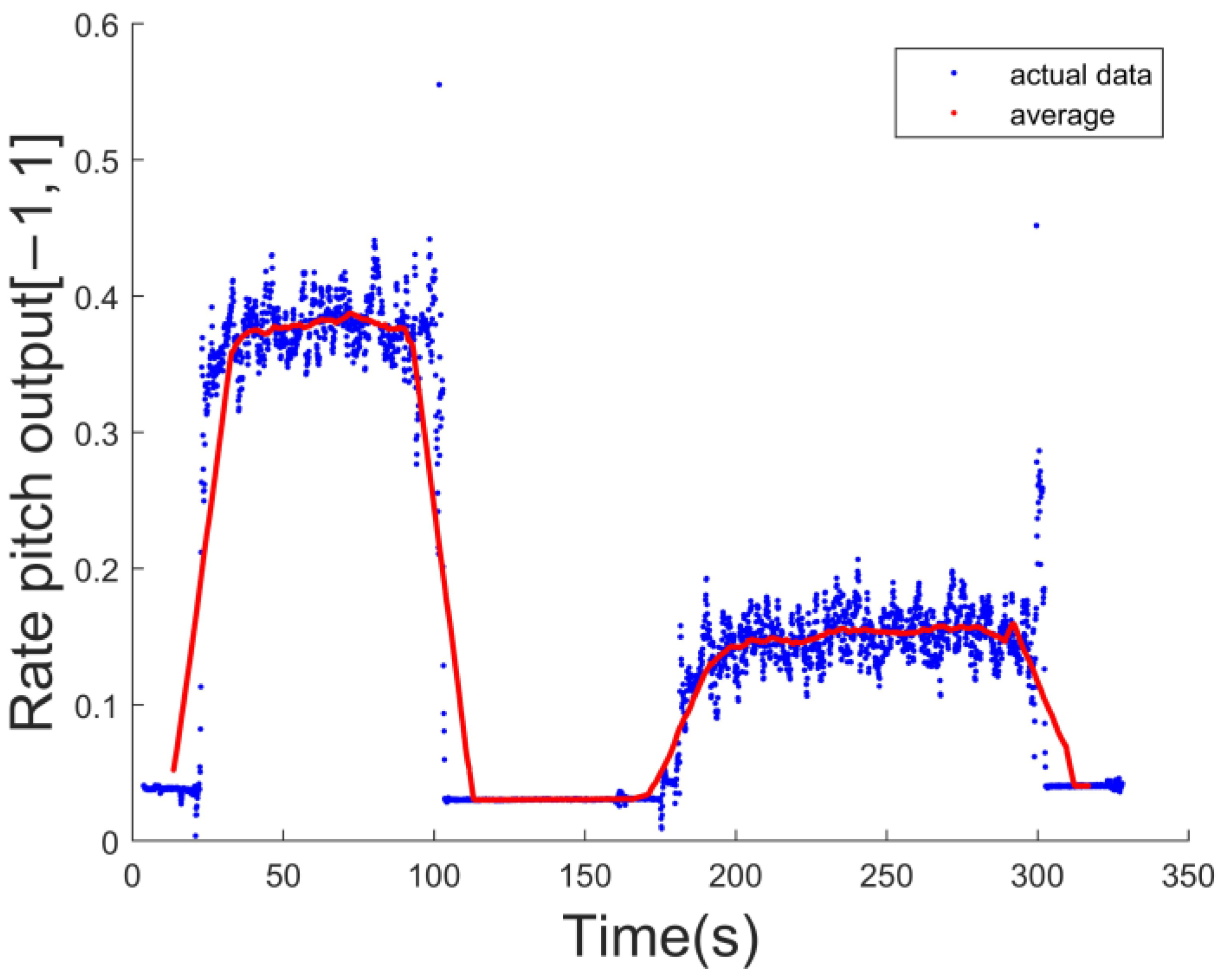
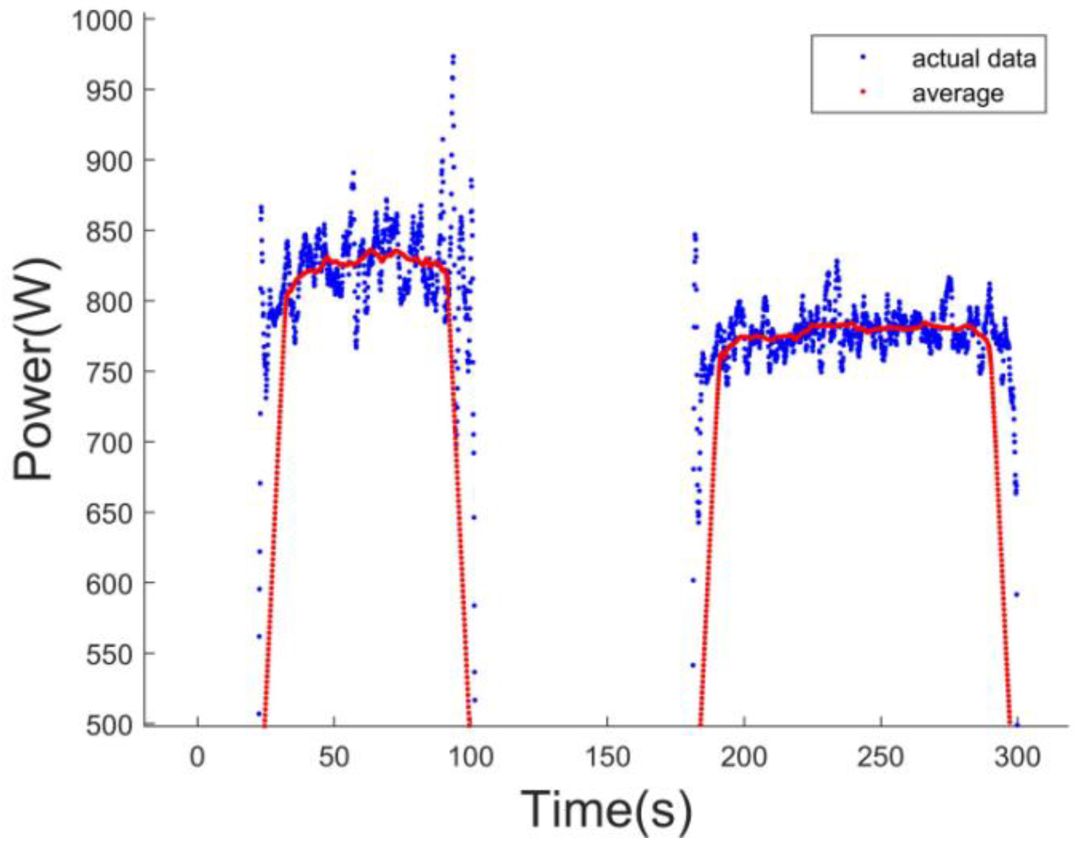
4.2. Bionic Power Optimization Experiments

As shown in Figure 14, the robot (LAWCDR) includes a Robomaster M2006 front wheel motor, four JuFeng 2814 kv700 motors, four 40A ESCs, four APC1055 propellers, a 60 mm double-layer nitrile rubber suction cup, and two Feetech SM45BL RS485 servos. The flight controller is CUAV fmuv5 nano flight controller. The wheel diameter is 14 cm. The onboard computer is Nvidia Jetson Xavier NX, through the mavlink protocol and ROS for planning trajectory.

As shown in Figure 15, the robot position feedback indoors is output through the Optitrack motion capture system and sent to the robot through the Xbee communication module. The outdoor position feedback is output via differential GPS and the RTCM differential data from the base station is sent to the robot via Xbee as well. The robot performs position decomposition to obtain outdoor position feedback.

To verify the power optimization effect of the robot, we tested the power and control amount of the robot in different operating states when the robot was hovering in the air. The angular velocity control output of the pitch channel in the preparation state and flight state is shown in Figure 16. To better illustrate the variation, mean filtering of n = 200 was performed (shown as the red line). The control of the pitch axis is normalized to [–1,1]. In order to balance the non-coincidence of the center of gravity and geometric center, the robot needs to reduce the control margin of the pitch axis. From the preparation state to the flight state, the amount of control is reduced from 0.38 to 0.15, and the control margin is increased from 0.62 to 0.85. This causes an increase of 37.1% in the control margin. Compared to the preparation state, the flight state increases the control margin and improves the control performance of the robot.

The total robot power is shown in Figure 17. We also performed the mean filtering with n = 200 (as shown in the red line). The total robot hovering power is about 830 W when the robot is in the preparation state and about 780 W when the robot is in the flight state. The power difference is about 6%. If the robot works in the flight state, the working time of the robot can be extended. Taking a 6 s 5000 mah battery as an example, the robot working time can be extended from 481 s to 512 s.

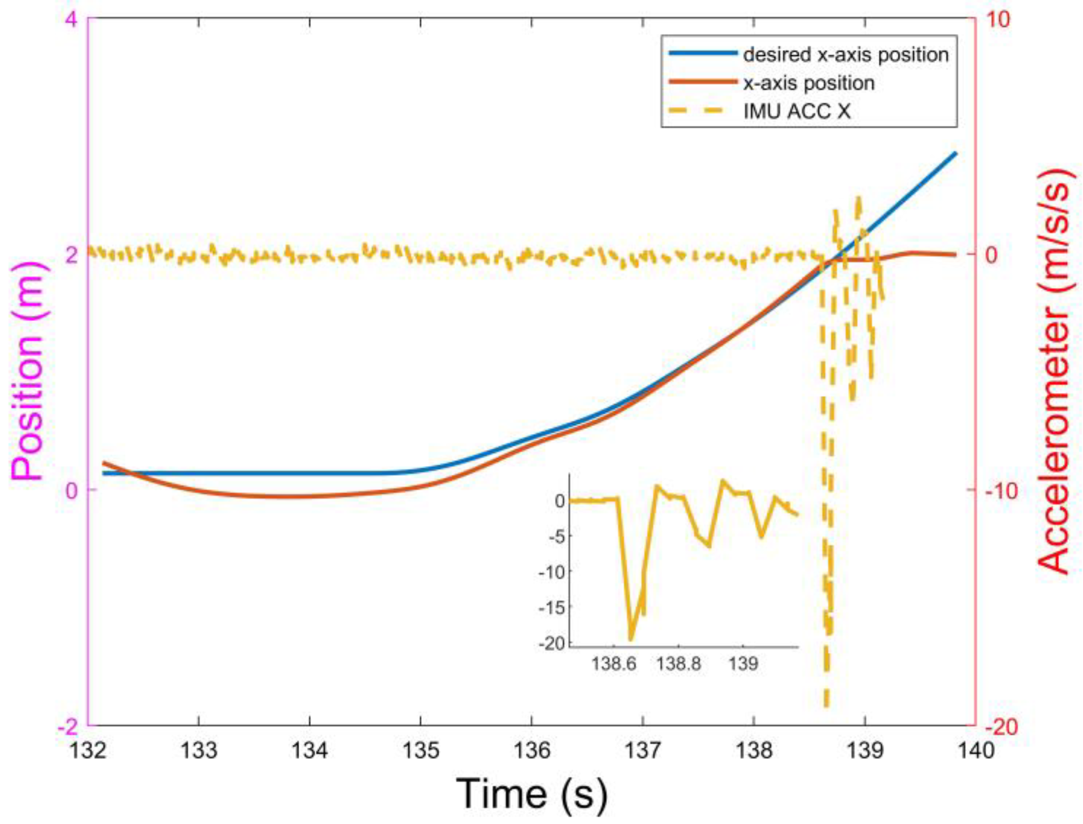
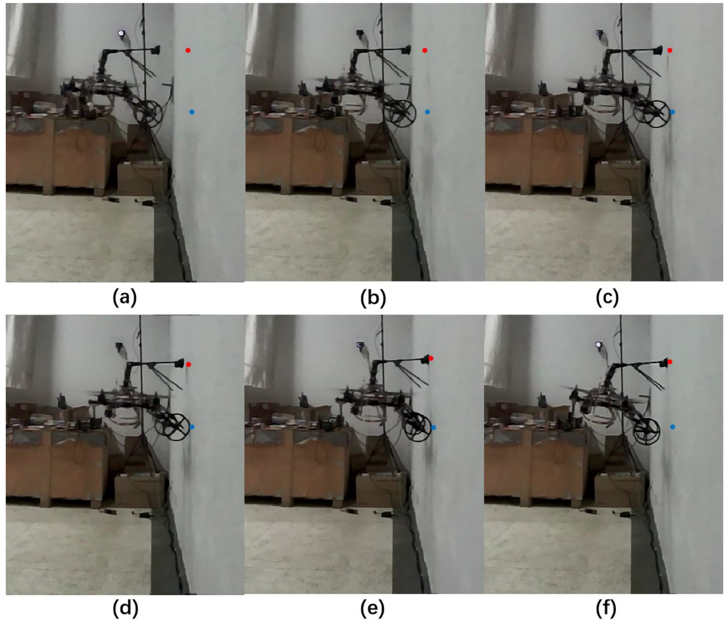
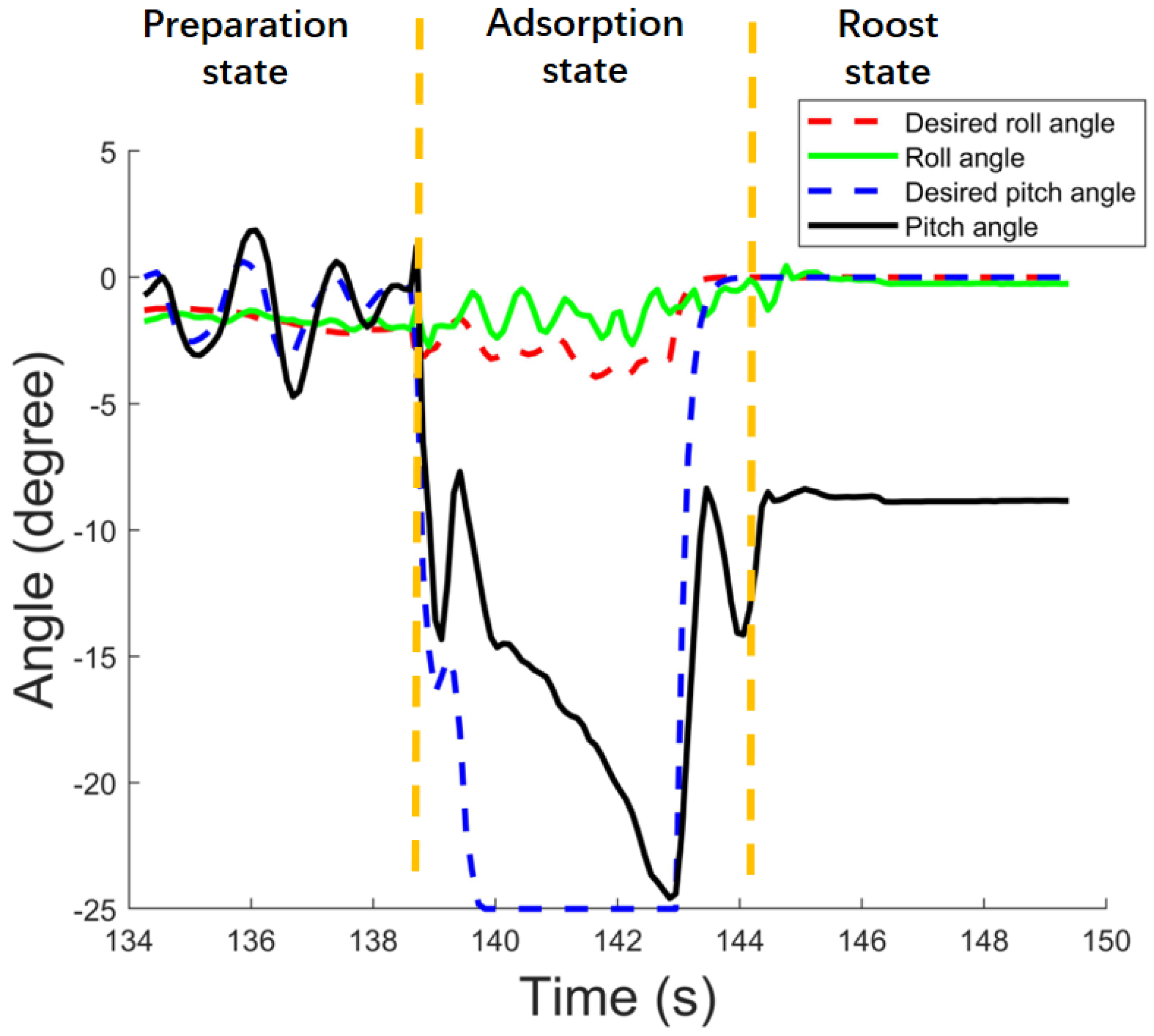
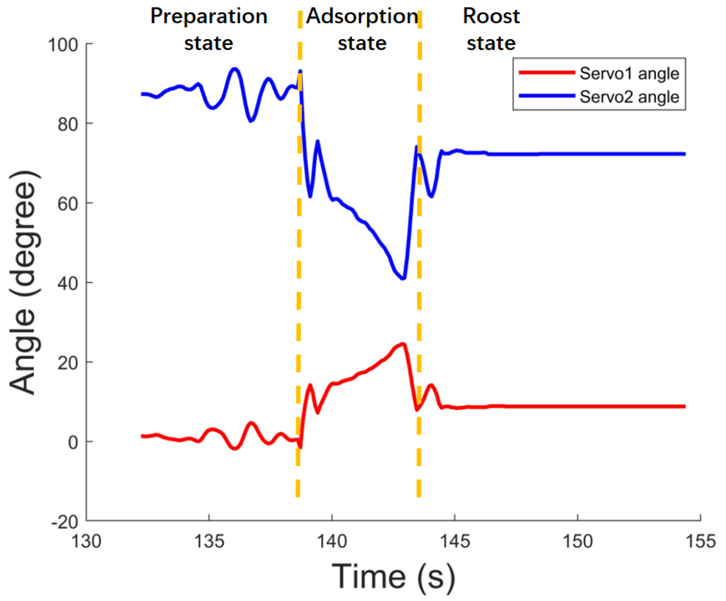
4.3. Actual Motion Process Experiments (Including Bionic Adsorption)

The main working state transitions of the robot (LAWCDR) are air–wall transformation and land–air transformation. The air–wall transformation process includes the flight adsorption process and the inverse process. The robot takes off from the ground, hovers at a height of 1 m, flies to the front of the wall, and performs flight adsorption. Firstly, the robot adjusts the servos to the preparation state to reduce the reaction time of performing the adsorption action. Secondly, the robot adjusts its heading to face the wall. Thirdly, the robot flies toward the wall at a slow, desired speed. When the wheels contact the wall, the shock absorbers are compressed to further adjust the robot’s heading. Fourthly, the flight control detects the contact. The servos horizontally stretch out the suction cup to contact the wall and the robot finally completes the flight adsorption process.

The robot performs a fast contact detection through the IMU. Once the acceleration of the x-axis that exceeds a threshold momentarily is detected, the robot controls the servos to start moving from the preparation position and stretches out the suction cup to contact the wall. As shown in Figure 18, after 138 s, the robot contacts the wall, and the actual position of the robot reaches 2 m without further change (as shown in the red line). The x-axis acceleration (as shown in the yellow line) steps from 0 to 20 m/s/s, exceeding the threshold value (8 m/s/s).

The robot imitates a gecko for adsorption as shown in Figure 19, where (a) the robot is hovering in the air and the suction cup moves to the preparation state for adsorption. (b) The robot starts to fly toward the wall. (c) The front wheels start to contact the wall (the contact point between the right wheel and the wall is the blue point). The shock absorbers start to work, adjusting the robot’s heading. (d) The suction cup driven by the servos moves towards the painted wall. As shown in Figure 19e,f, the suction cup contacts the wall (the contact point between the suction cup and the wall is the red point) and a negative pressure environment is established.

As shown in Figure 20, the robot adjusts the desired attitude angle from 0 degrees to −25 degrees after contact is detected at 138 s. The desired and actual roll angles remain at about 0 degrees. The actual pitch angle changes from 0 to −25 degrees, and a horizontal component force is applied to the wall. This assures that the wheels are attached to the wall before the suction cup contacts the wall. During the roost state, the desired pitch angle is 0 and the rotors stop working. The actual pitch angle of the robot is kept at −10 degrees due to gravity.

The angle curves of servo 1 and servo 2 during the adsorption process are shown in Figure 21. When the contact is detected, the angle of servo 1 changes from 0 degrees to 24.5 degrees. The angle of servo 2 changed from 93 degrees to 41 degrees. Therefore, the servos keep horizontally stretching out the suction cup to contact the wall.

The trajectory of the land and air transformation process of the robot is shown in Figure 22. The experiment to verify the land–air motion movement capability of the robot was carried out. The robot follows a planned trajectory of ground motion, air flight, takeoff, and landing. The robot moves from point A to point B, takes off at point B and moves to air point C, then flies through points D and E to point F, lands at point G, and then moves to points H and I on the ground. The entire movement process is completely autonomous.

5. Conclusions

This paper develops a land–air–wall cross-domain robot that combines the advantages of the land–air amphibious robot and the flying adsorption amphibious robot and imitates the process of geckos using their spines to complete adsorption again after collision with the wall. The robot imitates the bionic adsorption process and uses servos and shock absorbers to simulate the spine. In addition, inspired by the phenomenon of geckos adjusting their attitude in the air for a smooth landing, we adjust the position of the suction cup and servos in the air and coincide the center of gravity of the robot with the geometric center as much as possible, which reduces the power consumption and improves the efficiency during flight. The experiment and simulation results demonstrate that the robot can work properly in three environments and complete air–wall transformation and land–air transformation. By adjusting the robot’s center of gravity, it is possible to save up to 6% of power consumption and improve the control margin.

References

1. Liu, Y.; Sun, G.; Chen, H. Impedance control of a bio-inspired flying and adhesion robot. In Proceedings of the 2014 IEEE International Conference on Robotics and Automation (ICRA), Hong Kong, China, 31 May–7 June 2014; pp. 3564–3569. [Google Scholar] [CrossRef]
2. Kossett, A.; Purvey, J.; Papanikolopoulos, N. More than meets the eye: A hybrid-locomotion robot with rotary flight and wheel modes. In Proceedings of the 2009 IEEE/RSJ International Conference on Intelligent Robots and Systems, St. Louis, MO, USA, 10–15 October 2009; pp. 5653–5658. [Google Scholar] [CrossRef]
3. Kossett, A.; D’Sa, R.; Purvey, J.; Papanikolopoulos, N. Design of an improved land/air miniature robot. In Proceedings of the 2010 IEEE International Conference on Robotics and Automation, Anchorage, AK, USA, 3–7 May 2010; pp. 632–637. [Google Scholar] [CrossRef]
4. Kossett, A.; Papanikolopoulos, N. A robust miniature robot design for land/air hybrid locomotion. In Proceedings of the 2011 IEEE International Conference on Robotics and Automation, Shanghai, China, 9–13 May 2011; pp. 4595–4600. [Google Scholar] [CrossRef]
5. Kalantari, A.; Spenko, M. Design and experimental validation of HyTAQ, a Hybrid Terrestrial and Aerial Quadrotor. In Proceedings of the 2013 IEEE International Conference on Robotics and Automation, Karlsruhe, Germany, 6–10 May 2013; pp. 4445–4450. [Google Scholar] [CrossRef]
6. Meiri, N.; Zarrouk, D. Flying STAR, a Hybrid Crawling and Flying Sprawl Tuned Robot. In Proceedings of the 2019 International Conference on Robotics and Automation (ICRA), Montreal, QC, Canada, 20–24 December 2019; pp. 5302–5308. [Google Scholar] [CrossRef]
7. Huang, C.; Liu, Y.; Ye, X. Design, simulation and experimental study of a force observer for a flying&ndash;perching quadrotor. Robot. Auton. Syst. 2019, 120, 103237. [Google Scholar] [CrossRef]
8. Wopereis, H.W.; Molen, T.D.v.d.; Post, T.H.; Stramigioli, S.; Fumagalli, M. Mechanism for perching on smooth surfaces using aerial impacts. In Proceedings of the 2016 IEEE International Symposium on Safety, Security, and Rescue Robotics (SSRR), Lausanne, Switzerland, 23–27 October 2016; pp. 154–159. [Google Scholar] [CrossRef]
9. Thomas, J.; Pope, M.; Loianno, G.; Hawkes, E.W.; Estrada, M.A.; Jiang, H.; Cutkosky, M.R.; Kumar, V. Aggressive flight with quadrotors for perching on inclined surfaces. J. Mech. Robot. 2016, 8, 051007. [Google Scholar] [CrossRef]
10. Kalantari, A.; Mahajan, K.; Ruffatto, D.; Spenko, M. Autonomous perching and take-off on vertical walls for a quadrotor micro air vehicle. In Proceedings of the 2015 IEEE International Conference on Robotics and Automation (ICRA), Seattle, WA, USA, 25–30 May 2015; pp. 4669–4674. [Google Scholar] [CrossRef]
11. Liu, Z.; Karydis, K. Toward impact-resilient quadrotor design, collision characterization and recovery control to sustain flight after collisions. In Proceedings of the 2021 IEEE International Conference on Robotics and Automation (ICRA), Xi’an, China, 30 May–5 June 2021; pp. 183–189. [Google Scholar] [CrossRef]
12. Chui, F.; Dicker, G.; Sharf, I. Dynamics of a quadrotor undergoing impact with a wall. In Proceedings of the 2016 International Conference on Unmanned Aircraft Systems (ICUAS), Arlington, VA, USA, 7–10 June 2016; pp. 717–726. [Google Scholar] [CrossRef]
13. Dicker, G.; Chui, F.; Sharf, I. Quadrotor collision characterization and recovery control. In Proceedings of the 2017 IEEE International Conference on Robotics and Automation (ICRA), Singapore, 29 May–3 June 2017; pp. 5830–5836. [Google Scholar] [CrossRef]
14. Battiston, A.; Sharf, I.; Nahon, M. Attitude estimation for normal flight and collision recovery of a quadrotor UAV. In Proceedings of the 2017 International Conference on Unmanned Aircraft Systems (ICUAS), Miami, FL, USA, 13–16 June 2017; pp. 840–849. [Google Scholar] [CrossRef]
15. Dicker, G.; Sharf, I.; Rustagi, P. Recovery control for quadrotor UAV colliding with a pole. In Proceedings of the 2018 IEEE/RSJ International Conference on Intelligent Robots and Systems (IROS), Madrid, Spain, 1–5 October 2018; pp. 6247–6254. [Google Scholar] [CrossRef]
16. Liu, Y.; Chen, H.; Tang, Z.; Sun, G. A bat-like switched flying and adhesive robot. In Proceedings of the 2012 IEEE International Conference on Cyber Technology in Automation, Control, and Intelligent Systems (CYBER), Bangkok, Thailand, 27–31 May 2012; pp. 92–97. [Google Scholar] [CrossRef]
17. Tanaka, K.; Spenko, M. A gecko-like/electrostatic gripper for free-flying perching robots. In Proceedings of the 2020 IEEE Aerospace Conference, Big Sky, MT, USA, 7–14 March 2020; pp. 1–7. [Google Scholar] [CrossRef]
18. Daler, L.; Klaptocz, A.; Briod, A.; Sitti, M.; Floreano, D. A perching mechanism for flying robots using a fibre-based adhesive. In Proceedings of the 2013 IEEE International Conference on Robotics and Automation, Karlsruhe, Germany, 6–10 May 2013; pp. 4433–4438. [Google Scholar] [CrossRef]
19. Roderick, W.R.T.; Cutkosky, M.R.; Lentink, D. Bird-inspired dynamic grasping and perching in arboreal environments. Sci. Robot. 2021, 6, 7562. [Google Scholar] [CrossRef] [PubMed]
20. Mehanovic, D.; Bass, J.; Courteau, T.; Rancourt, D.; Desbiens, A.L. Autonomous Thrust-Assisted Perching of a Fixed-Wing UAV on Vertical Surfaces; Springer: Cham, Switzerland, 2017; pp. 302–314. [Google Scholar] [CrossRef]
21. Thomas, J.; Polin, J.; Sreenath, K.; Kumar, V. Avian-Inspired Grasping for Quadrotor Micro UAVs. In Proceedings of the ASME 2013 International Design Engineering Technical Conferences and Computers and Information in Engineering Conference, Portland, OR, USA, 4–7 August 2013; Volume 6A, p. 55935. [Google Scholar] [CrossRef] [Green Version]
22. Mehanovic, D.; Rancourt, D.; Desbiens, A.L. Fast and efficient aerial climbing of vertical surfaces using fixed-wing UAVs. IEEE Robot. Autom. Lett. 2018, 4, 97–104. [Google Scholar] [CrossRef]
23. Siddall, R.; Byrnes, G.; Full, R.J.; Jusufi, A. Tails stabilize landing of gliding geckos crashing head-first into tree trunks. Commun. Biol. 2021, 4, 1–12. [Google Scholar] [CrossRef] [PubMed]
24. Kim, S.; Choi, S.; Kim, H.J. Aerial manipulation using a quadrotor with a two DOF robotic arm. In Proceedings of the 2013 IEEE/RSJ International Conference on Intelligent Robots and Systems, Tokyo, Japan, 3–7 November 2013; pp. 4990–4995. [Google Scholar] [CrossRef]
25. Liu, Y.C.; Huang, C.Y. DDPG-based adaptive robust tracking control for aerial manipulators with decoupling approach. IEEE Trans. Cybern. 2021, 99, 1–14. [Google Scholar] [CrossRef] [PubMed]
26. Jusufi, A.; Goldman, D.I.; Revzen, S.; Full, R.J. Active tails enhance arboreal acrobatics in geckos. Proc. Natl. Acad. Sci. USA 2008, 105, 4215–4219. [Google Scholar] [CrossRef] [PubMed] [Green Version]
27. Guo, B.Z.; Zhao, Z.L. On the convergence of an extended state observer for nonlinear systems with uncertainty. Syst. Control Lett. 2011, 60, 420–430. [Google Scholar] [CrossRef]
28. Zhao, Z.L.; Guo, B.-Z. Extended state observer for uncertain lower triangular nonlinear systems. Syst. Control Lett. 2015, 85, 100–108. [Google Scholar] [CrossRef]
29. Yue, M.; Liu, B.; An, C.; Sun, X. Extended state observer-based adaptive hierarchical sliding mode control for longitudinal movement of a spherical robot. Nonlinear Dyn. 2014, 78, 1233–1244. [Google Scholar] [CrossRef]
30. Pan, H.; Sun, W.; Gao, H.; Hayat, T.; Alsaadi, F. Nonlinear tracking control based on extended state observer for vehicle active suspensions with performance constraints. Mechatronics 2015, 30, 363–370. [Google Scholar] [CrossRef]
31. Abdul-Adheem, W.R.; Azar, A.T.; Ibraheem, I.K.; Humaidi, A.J. Novel active disturbance rejection control based on nested linear extended state observers. Appl. Sci. 2020, 10, 4069. [Google Scholar] [CrossRef]
Figure 1. The overall structure of the robot (LAWCDR).
Applsci 12 03988 g001
Figure 2. Structure and coordinates of the robot (LAWCDR).
Applsci 12 03988 g002
Figure 3. Four working states of the robot (LAWCDR). (a) Flight state. (b) Preparation state. (c) Adsorption state. (d) Roost state.
Applsci 12 03988 g003
Figure 4. Adsorption process of the robot (LAWCDR) compared with the gecko (rotor lift keeps the wheels fixed on the wall). (a) The wheels start to contact the wall. (b) The wheels are compressed. (c) The robot uses the lift force generated by the propeller to attach the wheels to the wall. (d) The suction cup and support bars are driven towards the wall. (e) The suction cup makes the robot adsorb to the wall. (f) The correspondence between geckos and robots.
Applsci 12 03988 g004
Figure 5. Diagram of the spring mechanism installed on the front wheels. The red circles represent rotating shaft, orange device is the shock absorber.
Applsci 12 03988 g005
Figure 6. Force analysis of the robot. (a) Force analysis of the approaching state (propellers are working). (b) Force analysis of the adsorbing state (propellers are not rotating).
Applsci 12 03988 g006
Figure 7. Structure of the suction cup and the support bars.
Applsci 12 03988 g007
Figure 8. Influence of angle α to the support force N 2 on absorbing module.
Applsci 12 03988 g008
Figure 9. Influence of the support bar angles θ s to the support force N 2 .
Applsci 12 03988 g009
Figure 10. Propeller lift and actual power test: (a) lift/power test bench (b) fitting curve between lift and power consumption.
Applsci 12 03988 g010
Figure 11. The robot balancing the center of gravity by adjusting the servo.
Applsci 12 03988 g011
Figure 12. Simulation of control quantity of robot pitch channel.
Applsci 12 03988 g012
Figure 13. Simulation on robot extended state observer.
Applsci 12 03988 g013
Figure 14. Robot platform (LAWCDR).
Applsci 12 03988 g014
Figure 15. Setup of the robot in the experiments.
Applsci 12 03988 g015
Figure 16. The output control quantity at preparation state and flight state.
Applsci 12 03988 g016
Figure 17. Total power at preparation state and flight state.
Applsci 12 03988 g017
Figure 18. Process of the IMU-detecting robot contacting the wall.
Applsci 12 03988 g018
Figure 19. Robot flight adsorption step diagram (the red point is the contact point between the suction cup and the wall, and the blue point is the contact point between the right wheel and the wall).
Applsci 12 03988 g019
Figure 20. Attitude curve of the robot. (The different working states are divided by the yellow dotted line).
Applsci 12 03988 g020
Figure 21. Servo angle curve of the robot. (The different working states are divided by the yellow dotted line).
Applsci 12 03988 g021
Figure 22. Actual land–air trajectory of the robot.
Applsci 12 03988 g022
Publisher’s Note: MDPI stays neutral with regard to jurisdictional claims in published maps and institutional affiliations.