1. Introduction
The systematic visual inspection of specimen’s morphological traits has a long history in biology, allowing divergent traits among species and populations of the same species to be defined and forming the field of morphometrics [
1,
2]. This inspection lately relies on digital images where landmarks are placed on diagnostic structures of the organism and their relative position and distance are measured [
3]. These manually placed landmarks provide some standardizations and automation of morphometrics analysis [
4]. Their application to the field of fish biology has been especially successful because, due to their bilateral symmetry, it is possible to capture biologically significant traits in a two-dimensional image [
5,
6,
7,
8]. Nevertheless, placing landmarks in pictures can be quite labor-intensive and it requires prior biological knowledge (e.g., [
4]). In this context, machine learning models can solve some of these limitations.
Since the publication of Alexnet [
9] and its successors (e.g., VGG16 [
10] or ResNet [
11]), convolutional neuronal networks (CNNs) became a standard model for computer vision tasks. In contrast to landmark-based approaches where scientists carefully place the landmarks on images, CNNs learn to extract features in order to fulfil a user-defined task. CNNs are frequently implemented to solve object recognition or object detection applications. In fish biology, these models were successfully used for fish recognition [
12,
13,
14,
15,
16,
17]. Nevertheless, convolutional neuronal networks are black boxes and are hard to interpret [
18]. Their behavior needs to be investigated after model training relying on prediction samples [
19,
20,
21,
22]. The latent explanatory factors learned by the CNN, which were previously discussed to be the key factor for reliable machine learning models [
23], still cannot be unveiled. This means that biological factors contributing to the results of a neuronal network-based model cannot be extracted and analyzed.
This is a strong shortcoming in contrast to landmark-based analysis, where the landmarks can be interpreted in a biological manner. The authors of [
24] compared landmark-based approaches to machine learning approaches for a Nile tilapia population classification task. The authors relied on supervised methods and found that the machine learning models, including CNNs, used image regions with no biological meaning that happened to be correlated with the specimen’s population. This effect is known as clever-Hans predictors [
18].
In contrast to the CNN-based approaches, the biological processing steps for visual diversity investigation differs. In geometric morphometry the landmarks are processed (e.g., generalized Procrustes analysis [
25]) and the results are interpreted statistically. From a machine learning perspective, these landmarks represent manually defined features. These landmarks were defined without a priori information such as the specimen’s location. However, the features learned by CNNs differ significantly and typically rely on a supervised training procedure. These learned features and the manually extracted landmarks cannot be discussed in the same way.
CNN features are typically learned using a priori information [
9,
10,
11]. These features must not have biological meaning and may not be representative of a population’s visual diversity [
18]. In order to obtain reliable results, unsupervised machine learning was reported as an alternative to supervised methods [
24,
26,
27]. Furthermore, to be able to compare machine learning-based visual diversity to landmark-based approaches, the feature extraction must be trained without a priori information in an unsupervised manner.
This study investigates the latent structure and visible diversity of populations in digital images unveiled by unsupervised machine learning models. We quantify the performance of the applied methods by measuring their capability to unveil known population clusters. These clusters were reported at the molecular genetic level [
28,
29,
30] or are known due to geographical separation.
Since they breed among each other and tend to be exposed to similar environmental conditions, individuals of the same population are likely to share morphological features. In this study, we propose an unsupervised machine learning-based visual diversity investigation pipeline which is compared to landmark-based approaches. From two image datasets showing Nile tilapia specimens, landmarks are manually extracted and unsupervised machine learning models are trained to obtain features for each specimen. We hypothesize that:
Hypothesis 1. The machine learning models learn biological meaningful features.
Hypothesis 2. These features have a higher relation to the actual population clusters in contrast to landmark-based approaches.
The former hypothesis is evaluated by a visual inspection of the learned features. The latter hypothesis is evaluated in two ways. Initially, hypotheses tests are performed to investigate the relation between the features as well as landmarks to the known population clusters. Furthermore, we propose a novel non-parametric test to investigate the unambiguity of the known clusters in the learned feature space as well as in the extracted landmarks.
The contribution of this study is the investigation of the expressiveness of machine learning models in a biological context and the comparison of the results to landmark-based approaches. The hypotheses of this study are evaluated based on two Nile tilapia datasets that originate from specimens from Ethiopia and Uganda. These datasets were previously analyzed. In [
24], the relation of populations from Ethiopia were investigated using supervised (deep) machine learning-based specimen classification. The authors were able to achieve a prediction accuracy above
. However, they showed that this accuracy was achieved using clever-Hans predictors, and the classifiers used biological uninformative parts of the image. Ref. [
5] investigated Nile tilapia specimens from Uganda relying on landmark-based methods. The authors discussed population differences and showed overlapping population distributions.
To evaluate the hypotheses of this study, two unsupervised machine learning models are implemented. We use the Bayesian Gaussian process latent variable model [
31] previously used for Nile tilapia images [
24] and plant recognition [
26]. Furthermore, we implement an unsupervised deep learning counterpart, namely a convolutional autoencoder [
32]. These two models were chosen due to reported success in a biological context.
The remaining part of this study is structured as follows.
Section 2 introduces the materials and methods used for the evaluation of the aforementioned hypotheses.
Section 3 describes the results obtained by applying the proposed pipeline. Afterwards, the results are discussed before
Section 5 summarizes this work.
2. Materials and Methods
To evaluate the research hypotheses of this study, two main strategies were implemented. Initially, the learned features were visualized and manually inspected. For this inspection, the existing biological knowledge represented by the proposed landmark positions was used. The biological explainability of all used models was investigated. For the purpose of this study, we defined the biological explainability as the ability of models to explain the reasoning process based on meaningful biological information. To this end, we used the explainability of generalized Procrustes analysis, relying on landmarks placed on specimens as the reference for biological explainability.
In addition to this visual inspection, the features and landmarks were investigated using hypothesis tests. Initially we used Spearman’s rank correlation tests to investigate the relation between the features as well as landmarks to the known population clusters. However, these tests do not compare the capability of the machine learning models and landmark-based approaches to identify visible information which is useful to unveil the actual population clusters. In this study, we aimed to measure the unambiguity of known population clusters relying on processed landmarks or features obtained by machine learning models. The performance of the unsupervised machine learning models in contrast to the landmark-based approaches was evaluated by comparing the unveiled cluster unambiguity. To investigate this unambiguity of the known clusters in the learned feature space as well as in the extracted landmarks, we proposed a novel and non-parametric test. For this test, we created several population cluster hypotheses and used a novel Bayesian extension of consensus clustering [
33] as well as the principle of self-similarity for the formulation of a Bayesian hypothesis test for population discriminability.
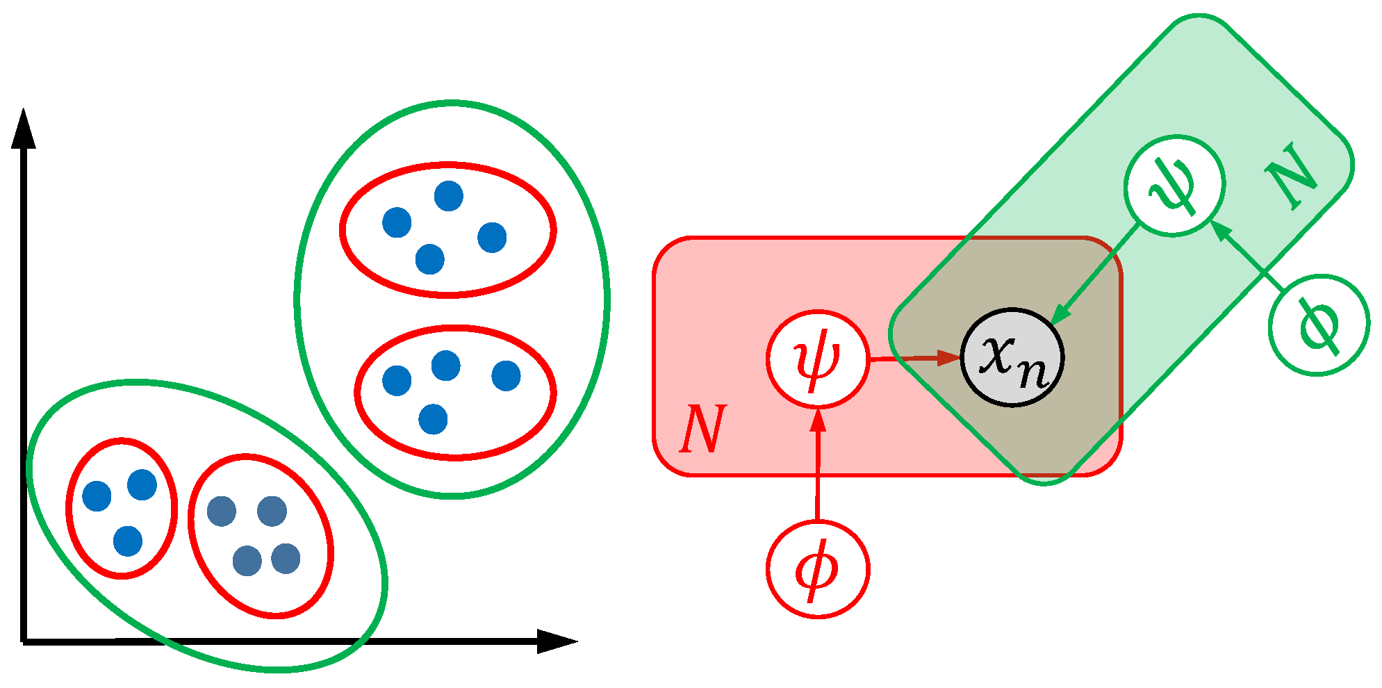
The technical core problem of this study was the quantification of a model’s capability to unveil morphological structure. However, this quantification is a complex task due to ambiguity. Different models and optimization strategies maybe result in biological meaningful morphological clusters using the same dataset [
29]. Similarly, a model may unveil subpopulations, but fail to quantify obvious differences in water bodies and vice versa. This effect is visualized in
Figure 1. On the left side, two dimensional representations of specimens (e.g., two principal coordinates of generalized Procrustes analysis features) are shown as blue points. The right side shows the visual representation of two models (red and green) with different global parameters
and local parameters
. Using different optimization strategies, two valid cluster hypotheses, namely four clusters (red model) or two clusters (green model) in the two-dimensional space, maybe occur.
Both cluster models unveil biological interpretable structures and may differ as a result of different mathematical formulations or optimization strategies. In order to be able to quantify methods, and inspired by infinite mixture models [
34] as well as the idea of cluster ensemble [
33,
35], this study combined multiple population structure hypotheses unveiled in landmark and machine learning-based visual diversity data. These visual diversity data were generated relying on generalized Procrustes analysis and unsupervised machine learning models. We aimed to fuse the information of all population structure hypotheses. The combined results, as well as known clusters, were used to compare the landmark-based approaches with the machine learning approaches.
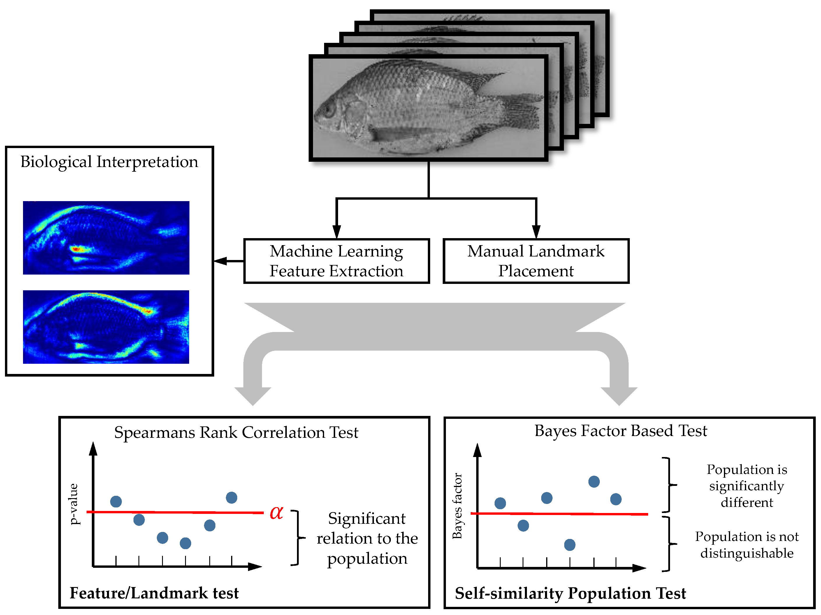
Our developed processing pipeline is shown in
Figure 2.
The remaining part of this chapter introduces the used data, landmark processing methods, machine learning models and morphological diversity investigation. The
Supplementary Materials (software as well as the used data including landmarks) is available under
https://github.com/TW-Robotics/MorphoML (accessed on 17 February 2022).
2.1. Data Sources
This study relied on two image datasets, namely from Ethiopia (209 images, six populations) and Uganda [
5] (462 images, 19 populations). All images were carefully gathered, prepared for digital processing and converted to grayscale images. The specimens in the images were cut out and resized to
pixels. A summary of the used image datasets is available in
Table 1.
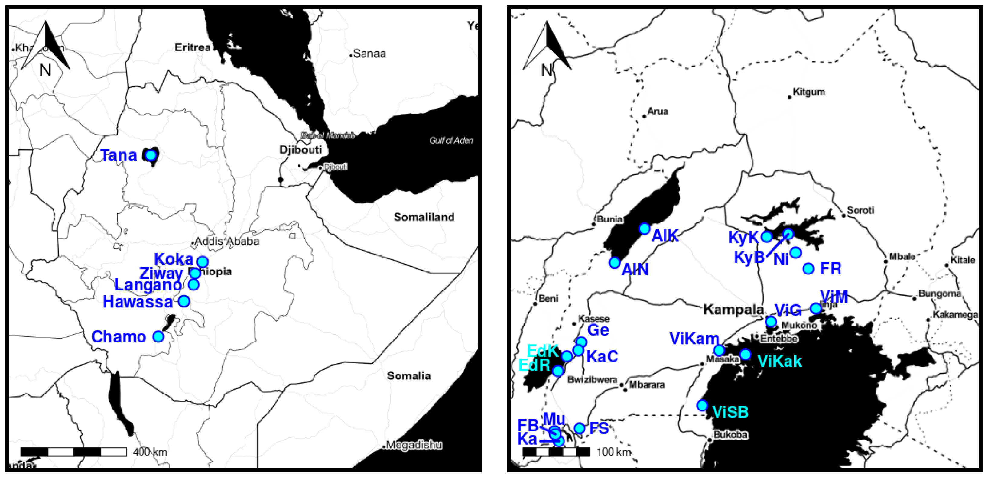
The population locations are visualized in
Figure 3.
For the purpose of this study, the locations of the specimens were used to quantify the capability of the models to unveil meaningful structure. This approach was motivated by the previous work of [
5,
24], where the authors showed morphological differences for populations of Uganda and Ethiopia. However, if visible differences did not exist our approach would fail and no meaningful structure could be extracted.
2.2. Visible Information Extraction
The image datasets from Uganda and Ethiopia were processed individually. We initially placed landmarks on the digital images and applied generalized Procrustes analysis (GPA) [
25]. To obtain features from the machine learning models, we used the Bayesian Gaussian process latent variable model (B-GP-LVM) [
31] previously used for Nile tilapia population classification [
24]. Motivated by the success of deep learning, we used a convolutional autoencoder (cAE) [
32] as a deep learning counterpart to the B-GP-LVM.
However, both machine learning models were based on image datasets of n gray-scaled images. Each image consists of R rows and C columns. The B-GP-LVM as well as the cAE tackles the problem of estimating a latent representation for the image . This latent representation is referred as feature. The models estimate the features for the specimens using different strategies and architectures. The features contain major information of the images and thus may represent visible characters representative of the populations.
2.2.1. Landmark Placement and Processing
The GPA relies on landmarks previously used for the Nile tilapia populations from Ethiopia [
24] as well as Uganda [
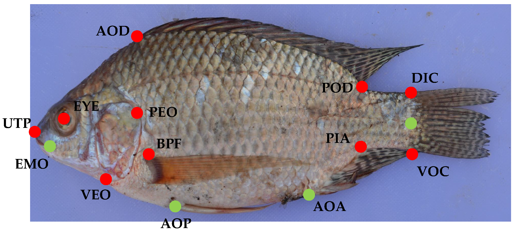
5]. 14 landmarks were used for Ethiopia and ten landmarks were used for Uganda. In order to investigate the impact of the number of landmarks, we used this different number of landmark positions for the images. The used landmark positions are shown in
Figure 4 as well as
Table 2.
OpenCV [
38] was used to place the landmarks on the specimens. The landmarks were processed using the GPA implementation in the cran R [
36] package
shapes [
39]. We used an F-test to investigate the relation between the Procrustes distances and the known specimen locations [
40,
41,
42,
43].
2.2.2. Bayesian Gaussian Process Latent Variable Model
A Gaussian process latent variable model (GP-LVM) [
44,
45] introduces a randomly initialized latent representation for each image sample and a set of approximated Gaussian processes [
46] to recreate the images. In an optimization procedure, the parameters of the Gaussian processes as well as the latent image representations are adapted to the data. Using GP-LVM for images [
47], each image
is interpreted as a vector
and the latent counterpart is a low-dimensional vector
. The GP-LVM defines
, which maps the features
to
. This mapping is performed using a set of sparse Gaussian processes [
46].
Since this mapping is intractable, the authors of [
31] proposed the Bayesian Gaussian process latent variable model. The authors used variational inference [
48], where the prior
was used to optimize
After optimization of Equation (
1), we interpreted
as features for the image
.
was obtained from the optimized Gaussian distribution in the latent space.
The number of features D as well as the number of auxiliary points used by the sparse Gaussian process are estimated using the log marginal likelihood and the step-wise procedure:
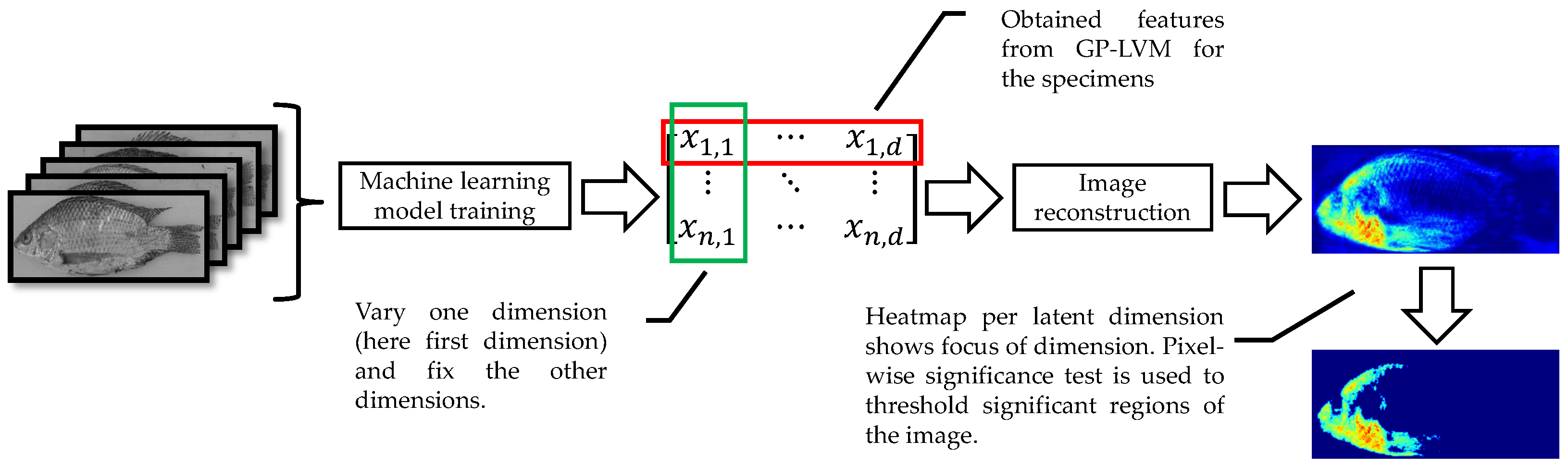
To visualize the visible characters learned by the B-GP-LVM, we applied the method of [
24,
47]. For this visualization of the
D features, we generated
n vectors
for each features. In this vector, we fixed all dimensions to the expectation except for the
d-th dimension, which was set to the true specimen value. Following this procedure,
n vectors for each feature could be generated. These vectors were projected to the image space. We calculated the pixel-wise variance and interpreted the resulting image as a visualization of the latent features space. For the interpretation of the images, we applied the pixel-wise hypothesis test for saliency maps (heatmaps) previously introduced in [
24]. The visualization procedure is visualized in
Figure 5.
We used the
GPy [
50] implementation of the B-GP-LVM relying on the radial base function (RBF) kernel including automatic relevance determination (ARD) [
51]. The models were initialized using the principal component analysis. The optimization was based on
sklearns L-BFGS-B optimizer [
52]. We used the default parameters and analyzed the log marginal likelihood at each 10th step. If the log marginal likelihood had not increased at a minimum of
, we aborted the optimization.
2.2.3. Convolutional Autoencoder
The GP-LVM learns features by optimizing the probabilistic mapping
, where
represents flattened images. This methodology can be interpreted as the generalization of the principal component analysis [
44]. An autoencoder (AE) [
53] is a (deep) neuronal network-based counterpart to the GP-LVM. For visual problems, the AE is typically extended using convolution layers in order to obtain spatial relations. This model is referred as a convolutional autoencoder (cAE).
A cAE estimates features relying on an architecture of artificial neurons. This architecture is based on an encoder part which extracts features using and an decoder part estimating and image reconstruction . During model training, a loss function is optimized. If this optimization converges, and the encoder extracts useful features for image reconstruction. These features are not guaranteed to be independent.
Our implementation is based on Keras [
54]. To this end, our encoder relies on the VGG-16 model [
10] and the decoder is based on the inverted structure of the encoders architecture. We used an ImageNet [
55] initialization of the encoder. The cAE was trained using the binary cross-entropy [
53] loss. The loss was optimized using ADAM [
56] implemented in Keras [
57]. The default parameters were used. We trained models with
features relying on five iterations. The training was stopped after 1000 epochs.
The model selection was implemented by investigating the last 50 epochs of the training and tackled the identification of an appropriate number of features. We applied a kernel density estimation relying on a Gaussian kernel. For each model, we extracted the maximum of the resulting density. We chose the model with the lowest maximum loss value obtained by the aforementioned procedure. Our model selection was implemented using the default kernel density estimation implementation in cran R [
36] using the default parameters.
For visualization, we proposed an adaption of the same principle described in
Section 2.2.2 for B-GP-LVM features. We fixed all elements in the feature vector to the mean value and varied the values for each dimension according to the obtained values. The vector was used to predict images using the decoder. We analyzed the pixel-wise variability of the obtained images.
2.2.4. Visual Interpretation of the Features
We obtained visual characters using the optimized B-GP-LVM as well as cAE. Nevertheless, both models reconstruct the image content using different strategies. This reconstruction includes background information (e.g., mounting frame) or location specific information (e.g., the mounting pin). As previously discussed by [
18,
24], machine learning algorithms may use biological uninformative image regions to obtain technical reasonable results. However, these image regions are not useful in the context of this study, where visible characters should be used to investigate the population’s structure.
We followed the procedure proposed in [
24] and carefully selected biological informative features manually. After model optimization and model selection, we visualized the learned features using the aforementioned methodology. All features containing non-biological information were rejected and not used for further investigation. The remaining features were analyzed using Spearman’s rank correlation test [
58], where for each feature we used
j and population
k :
There is no relation between feature j and the population k. For our visualization in the remaining part of this study, we showed
instead of the
p-value for the machine learning-based models.
2.3. Multivariate Data Analysis
The data investigation methods and models discussed above mainly focus on the GPA coordinate and feature visualization as well as statistical tests. Nevertheless the aim of this study is the investigation of the latent structure of the used methodologies. The data complexity and population correlation relying on multivariate analysis of extracted GPA coordinates as well as machine learning features was investigated and visualized. For this analysis, the GPA coordinates as well as the cAE features were reduced to three dimensions relying on the principal component analysis (PCA) ([
49], Chapter 12) as well as the fast independent component analysis (ICA) [
59,
60]. For the GP-LVM results, the first three independent dimension ranked relying on the relevance value of the kernel were used.
The visualization as well as correlation analysis was based on the
GGally R package [
61].
2.4. Investigation of Morphological Diversity
The application of the same models for structure investigation using the processed landmarks as well as the machine learning-based features may result in different population clusters. In genetics, this problem is tackled by seeking the optimal model using metrics such as cumulative ancestry contribution [
62] or the log marginal likelihood [
63,
64]. However, these numerical values must not be useful for the biological question, and several models may contain useful information about the visible diversity of the data. Furthermore, the numerical optimization may differ using different data pre-processing methods such as GPA or machine learning.
To be able to compare the results obtained by the landmark-based methods and machine learning-based methods, we created several structure hypotheses and sought consensus in these models. We argue that this consensus contains the morphological structure unveiled by multiple hypotheses. The comparison was performed using the fused hypotheses. In this study, we used Gaussian mixture model clustering [
49] relying on different numbers of possible clusters to generate data structure hypothesis. The cluster models were fused by extending consensus clustering [
33]. We empathize that any cluster model resulting in probability matrices may be used instead of Gaussian mixture models.
In the remaining subsections, the GPA scaled coordinates and machine learning features are referred to as “features”.
2.4.1. Visible Features Clustering and Population Structure Investigation
The proposed clustering method is based on the Gaussian mixture model (GMM) [
49]. The GMM is based on a set of
k multivariate Gaussian distributions. Each specimen
j represented by its features
is assigned to one of the
k clusters. The model is based on
The affiliation of a specimen feature
to the cluster
i is calculated by the variable
, which is a 1-of-K coded vector, and the conditional probability
During optimization, the parameters , , and are optimized. After optimization, we use the class probability as an estimate for specimen j belongs to the cluster .
We use the
mclust [
65] package relying on expectation maximization [
49] for optimization. For the investigation of the morphological structure,
k must be defined by the user. However, several strategies for
k optimization exist, e.g., the Bayesian information criterion [
66].
The optimization of the
k parameter is a fundamental problem in genetics as well. In genetics the marginal log-likelihood [
63], evidence lower bound [
48] or biological motivated criterion [
62] are used. Nevertheless, these optimization criteria are mainly focusing on technical parameters. Motivated by the facts,
That the used models may not be a good approximation for the unknown probability density functions,
The data are typically restricted as well as incomplete, and
Different
k’s may capture biological significant information on different scales [
67].
We hypothesize that by finding consensus in a set of reasonable cluster models relevant pattern representative for the overall population can be obtained.
2.4.2. Consensus Clustering
Finding consensus in several cluster models or clustering ensembles [
35] may be used to combine evidence unveiled by different models. The principle of co-association [
33] is a model-free methodology, where the consensus of several cluster models is found by analyzing the pairwise occurrence of samples in the same cluster in several partitions. The cluster model
i results in a partition
, where
is the m-th cluster in the n-th partition. All models results in the set
. The co-association (CA) of samples
j and
k relying on
m cluster models is measured by
The function returns 1 if both samples happens to be in the same cluster in partition . This methodology results in the co-association matrix, where the entries at is . After the investigation of all m clustering models, the co-association matrix contains a consensus about all models.
We propose a probabilistic extension of this method referred to as probabilistic co-association (pCA), where the cluster uncertainty is included. On one hand, this extension includes the probabilistic perspective of the structural investigation and allows on the other hand hypothesis testing. To investigate the pCA, the probabilistic formulation of Equation (
4) is the probability of two samples
m and
n happens to be in the same cluster
j of partition
p. This probability is calculated using
The variable
indicates the affiliation of sample
m to cluster
j in partition
p. Assuming that the
p cluster models are independent given the features, we can estimate the co-association
between sample
m and
n by
In this analysis, we assume that specimens belonging to the same population cluster happen to be in the same model cluster with a higher frequency as well as higher probability than specimens from different clusters. We visualize the conditional probability of in a matrix referred as the pCA matrix. Specimens that happen to be frequently in the same cluster appear bright in the entries of the pCA matrix.
Finally, the performance of the probabilistic consensus clustering for morphological data is evaluated. This evaluation is performed by analyzing the population intra co-association to the inter co-association. In a biological context, this analysis investigates the visual similarity of the specimens to the true population location and foreign population locations. We formulate a hypothesis test relying on the Bayes factor [
68], where we evaluate the probabilistic consensus of inter-population specimens. The intra co-association is measured by analyzing the similarity of a specimen
to all members of the location
using the pCA. The inter location co-association is measured by analyzing the similarity
to all specimens belonging to another location. If the method used for visual information extraction results in useful information, the intra co-association will exceed the inter co-association. Note, that we use a priori knowledge in this test, namely the known specimen population location. The test is implemented using
The index describes all members of the populations location without the actual specimen i of the population. Hence, we do not compare the visual similarity of the specimen to itself.
The evaluation of our hypothesis
:
The locations morphological structure significantly differs from the other locations for the location
and given model (GPA, B-GP-LVM or cAE) relies on the Bayes factor. We found significant morphological differences (e.g., accept the hypothesis) between a location
and the remaining specimens if
[
68].
Our method was implemented in cran R [
36]. For numerical stability, we analyzed the log of
as well as
instead of raw probabilities. We analyzed
cluster partitions for Ethiopia and Uganda. To avoid numerical instabilities, we added a uniform distributed jitter using
, which is the probability of
to
that the specimens are in the same population.
3. Experimental Results
This section initially provides insight into information extracted relying on the landmark-based approach and machine learning models. Afterwards, the structure investigation as well as the result of the hypothesis test are presented.
3.1. Visible Diversity Relying on Landmarks
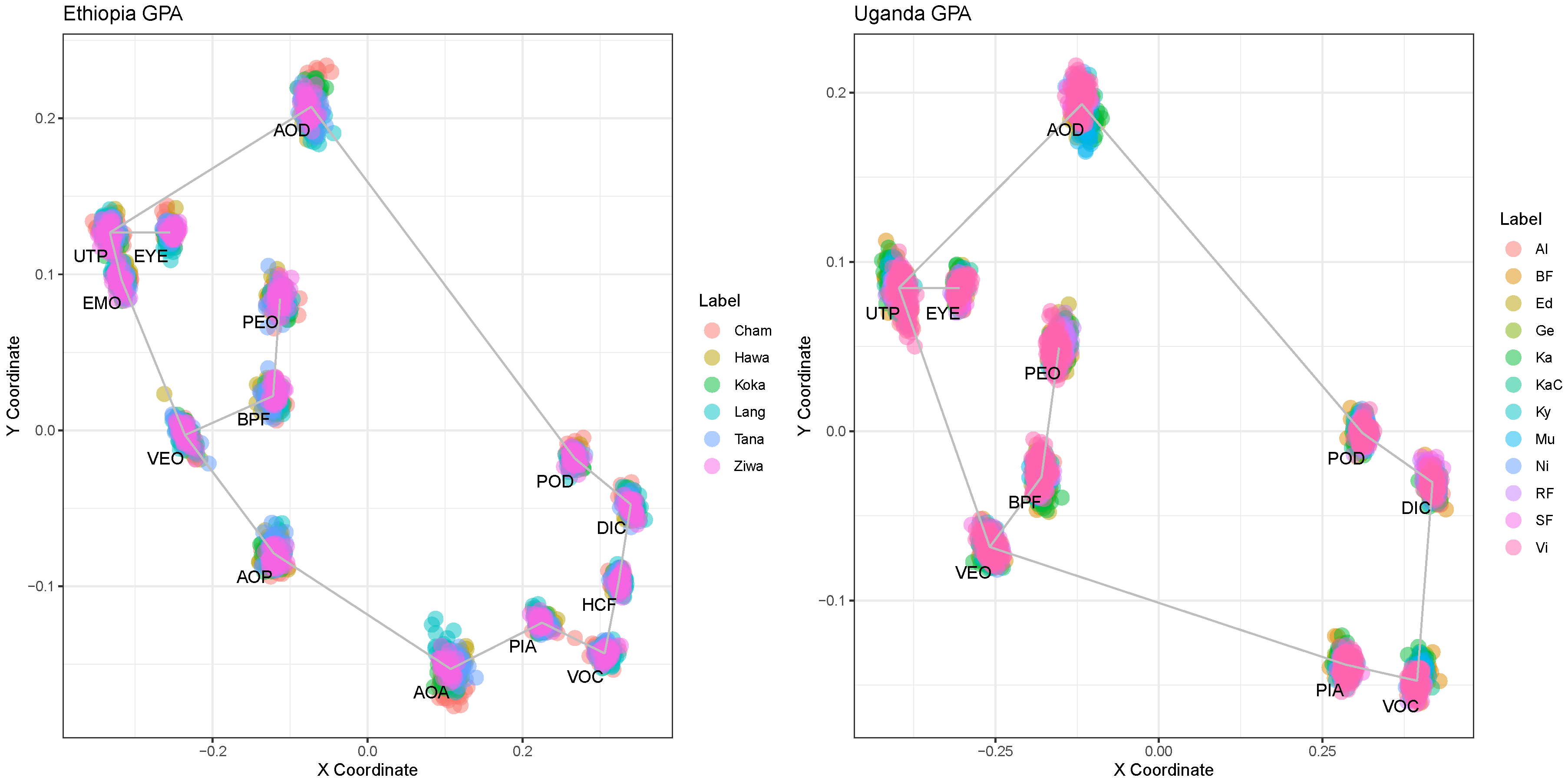
The landmarks were manually placed on the digital images. Analysis for specimens from Ethiopia was based on 14 landmarks, while for specimens from Uganda it was performed with ten landmarks. The result of the GPA feature scaling is illustrated in
Figure 6. For the purpose of visibility and readability, the water bodies of Victoria, Albert, Edward and Kyoga were visualized together.
An F-test for the investigation of the relation of the population to the coordinates relying on the Procrustes distance [
40,
41,
42,
43] showed significant relations between the locations and the Procrustes distance with a
p-value below
for both datasets.
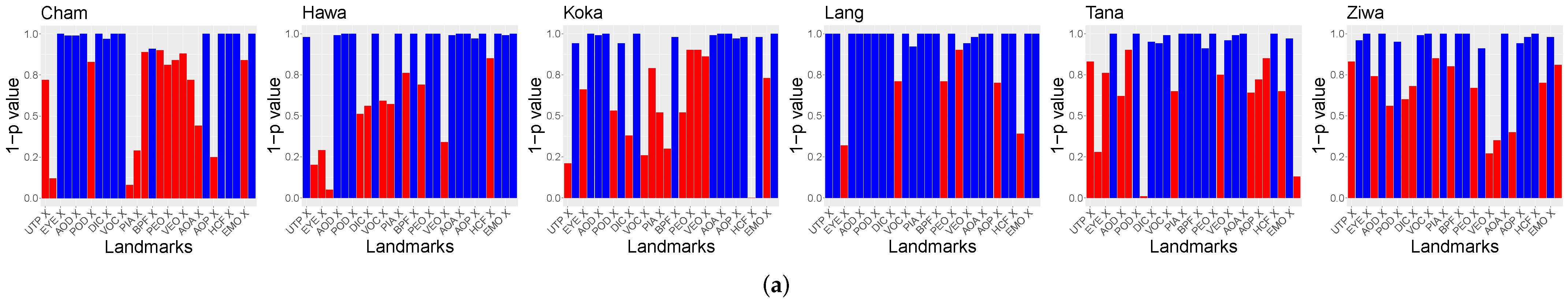
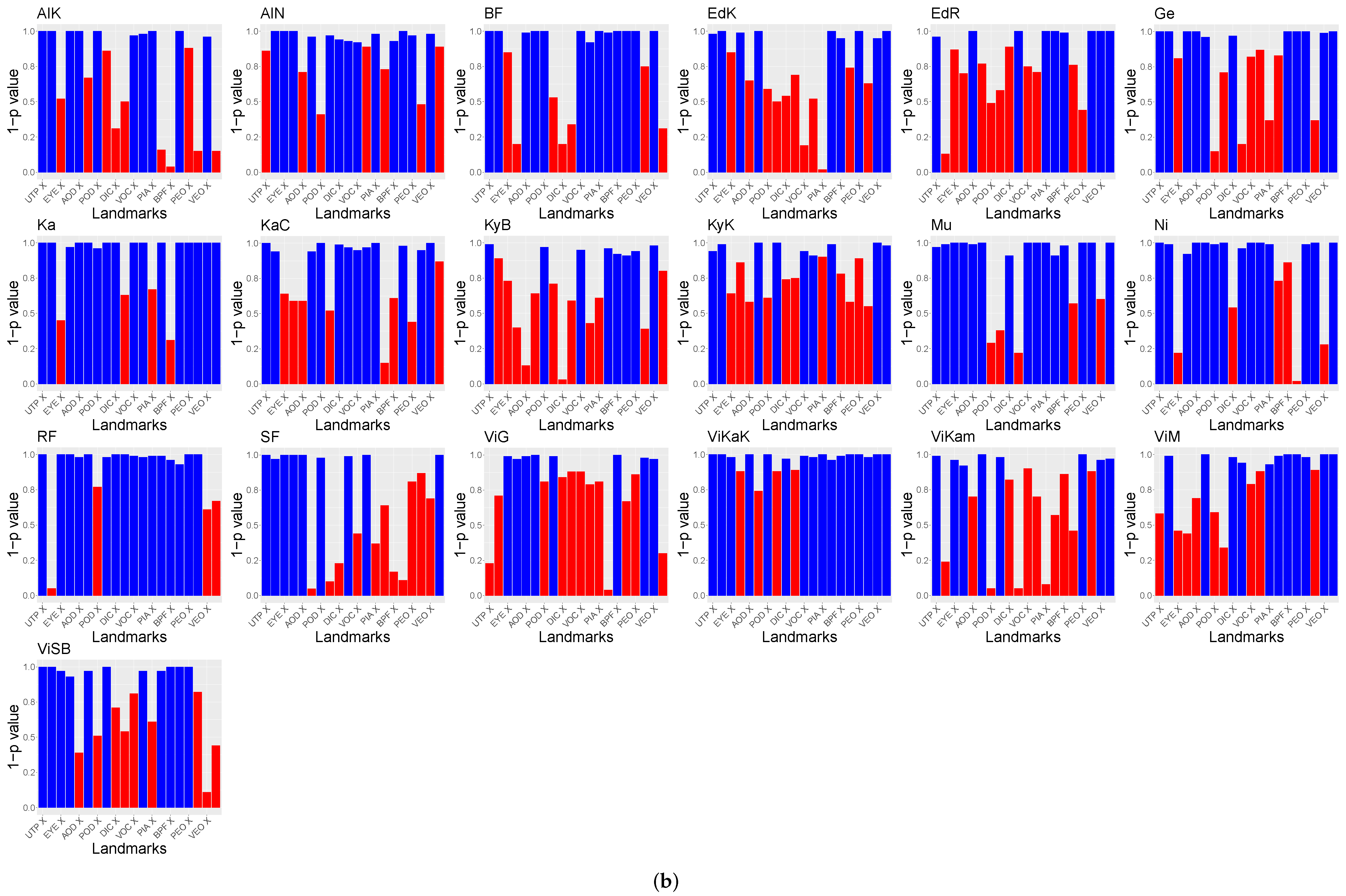
Furthermore, the relation of the X and Y coordinates of the landmarks to the population locations was tested. The
p-values of Spearman’s rank correlation test are visible in
Figure 7. For the purpose of visibility,
is shown. Landmarks above
are visualized in red.
The hypothesis test results indicate that there are significant relations between the X and Y GPA coordinates and the locations of the populations. No differences between the usage of ten or 14 landmarks were found. However, these tests did not unveil the differences between the populations relying on the GPA data.
3.2. Visible Diversity Relying on Machine Learning Models
This section presents the results of the learning procedures as well as the visualization and biological interpretation of the feature vectors.
3.2.1. Gaussian Process Latent Variable Model
The GP-LVM was optimized using the aforementioned procedure. This optimization approach resulted in 125 features as well as 200 auxiliary points for Ethiopia and 50 features as well as 125 auxiliary points for Uganda. Afterwards, noisy features and all features focusing on background information such as mounting pins or specimen fixtures were removed using a visual inspection of the features. After this manual procedure, 26 features for Ethiopia and 22 for Uganda remained in the feature set.
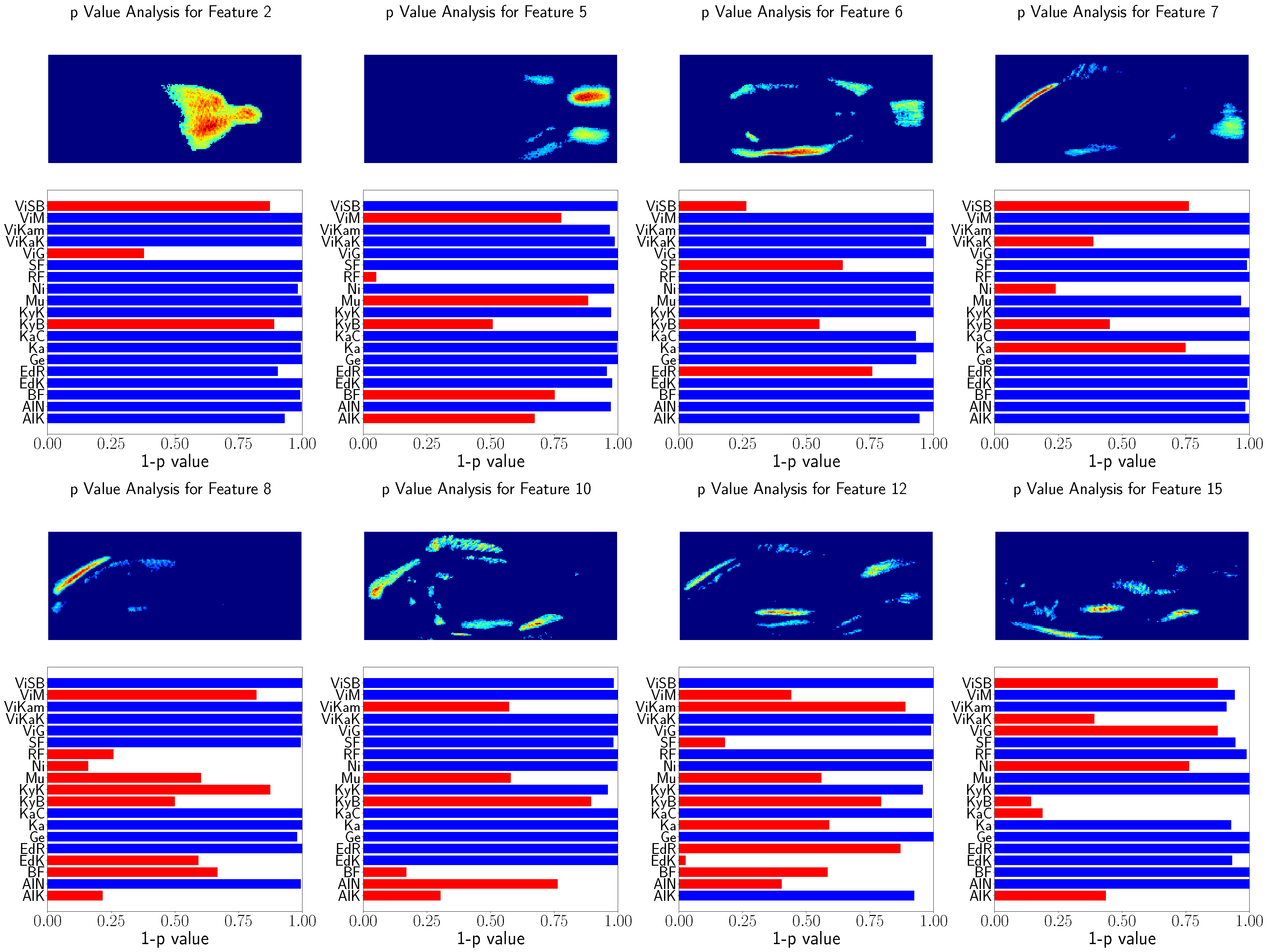
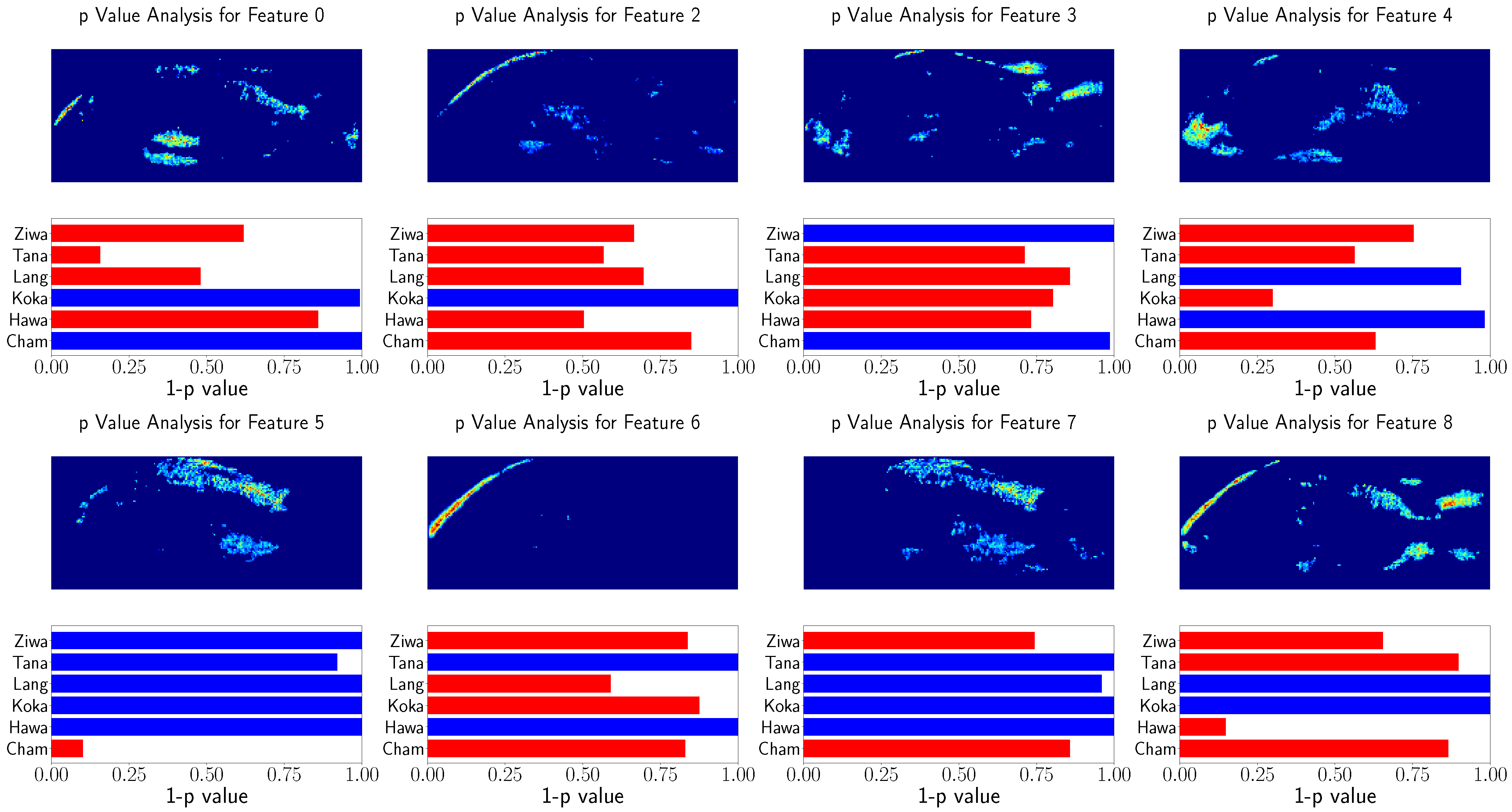
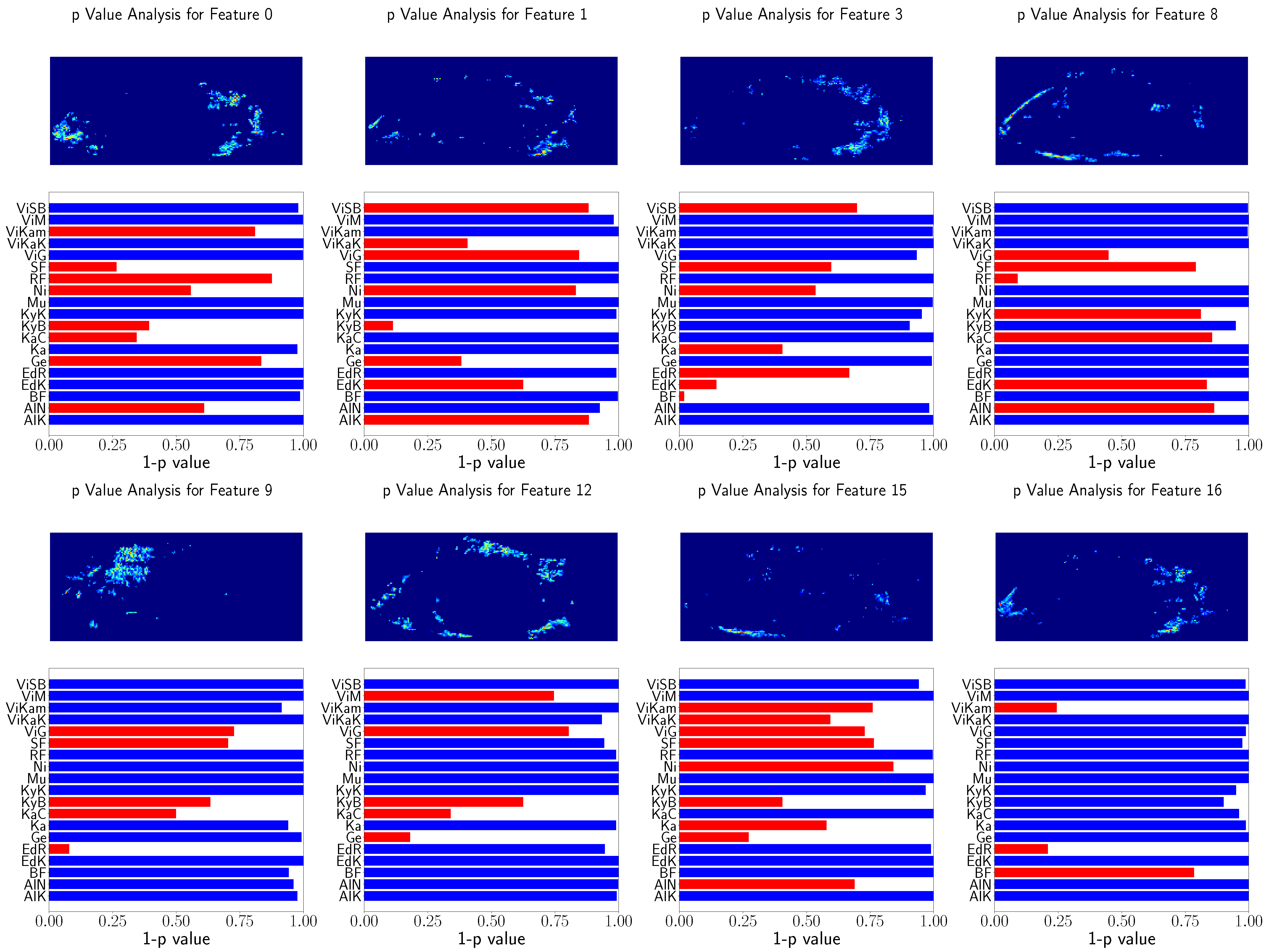
The relation of the remaining features to the population’s locations were tested using Spearman’s rank correlation test. The results of these tests as well as the visualization of the used features are shown in
Figure 8 and
Figure 9. This visualization shows the eight GP-LVM features with the highest ARD value of the optimized kernel. For better visualization
is visualized instead of the
p-value. The features above
are indicated with red bars.
The analysis of both datasets results in similar image regions. These image regions are in a similar position as the landmarks used for GPA. However, in contrast to the GPA coordinates, the heatmaps show the variability of image regions. While the GPA relies on the variability of discrete points, the GP-LVM analysis results in image regions in which the variability was tested to have a high relation to the population locations. The head and caudal fin region can clearly be seen in the visualization with a significant relation to the population’s location.
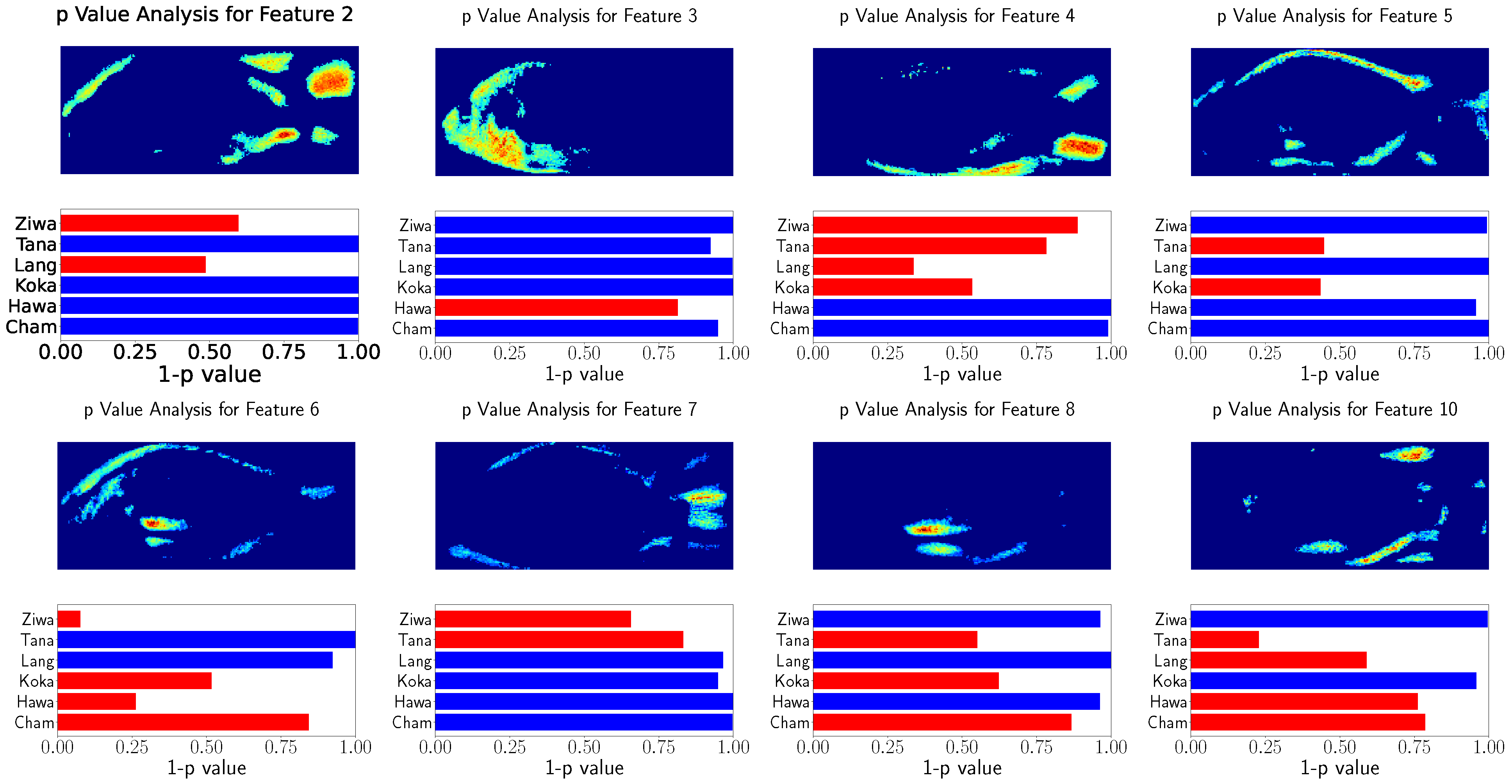
3.2.2. Convolutional Autoencoder
The optimization of the number of features used in the cAE was performed using the investigation of the loss after optimization discussed above. This optimization results in 25 features for Ethiopia and 100 features for Uganda. All extracted features were visualized relying on the GP-LVM feature visualization technique adapted for cAE [
26]. These features were manually investigated in a similar manner to the GP-LVM features. The selection procedure resulted in 23 features for Ethiopia and 46 features for Uganda. The number of features for Ethiopia was similar to the GP-LVM results. However, the number of features for Uganda exceeded the GP-LVM model selection.
Furthermore, the feature relation to the population location was tested using Spearman’s rank correlation test. This procedure is visualized in
Figure 10 and
Figure 11 for randomly selected features. Similarly, for better visualization
was is visualized instead of the
p value of Spearman’s rank correlation test, and the features above
are indicated with red bars.
Again, the heatmaps result in similar image regions used for GPA. However, the heatmaps are noisy and not as clear as the GP-LVM heatmaps. Nevertheless, the features show significant relation to the population locations.
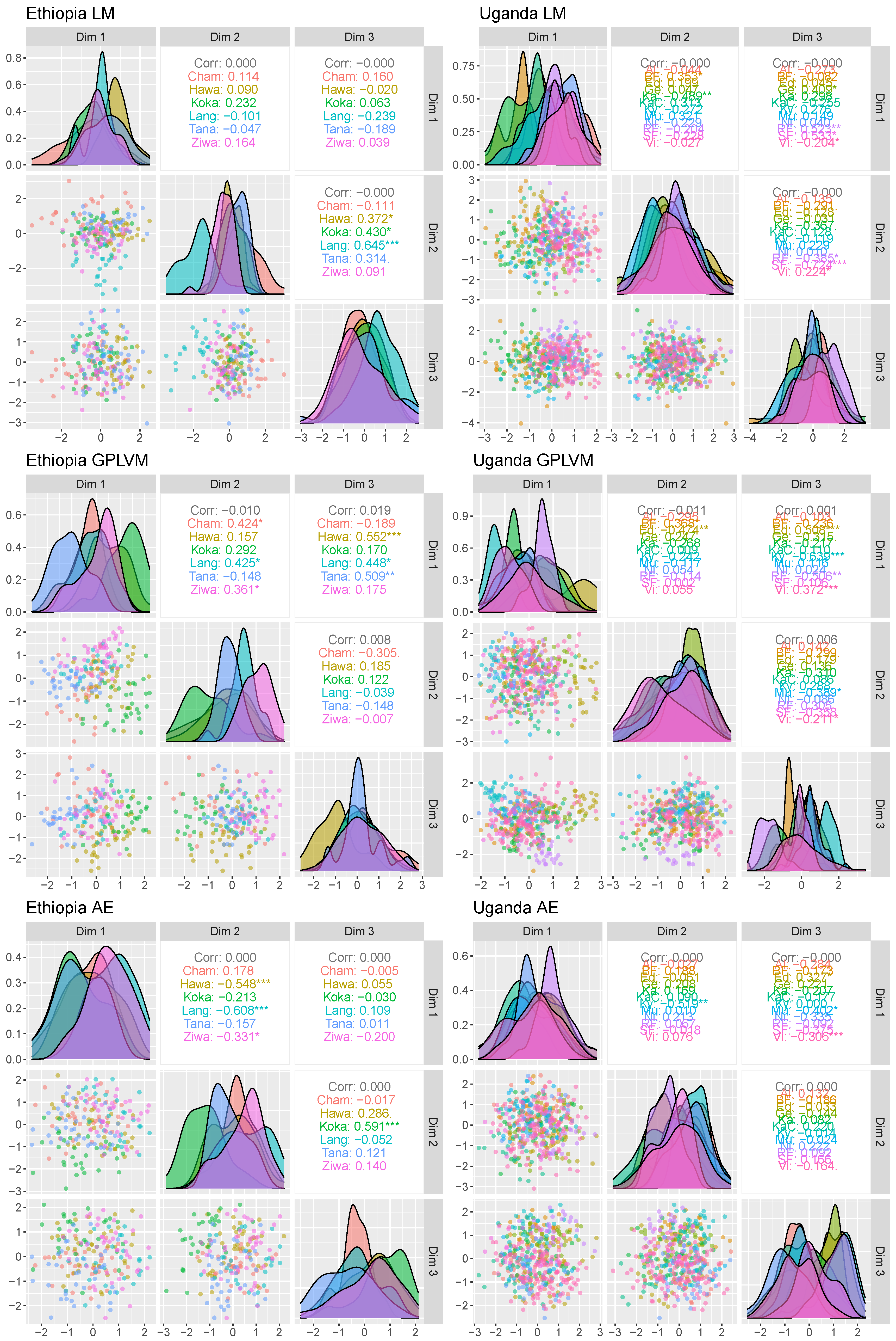
3.3. Multivariate Data Analysis
The multivariate analysis is shown in
Figure 12. All applied methodologies suffer from overlapping population locations. Nevertheless, several populations such as Tana, Langano or Chamo in Ethiopia do show different densities. However, relying on the presented low-dimensional data, no population location is separable.
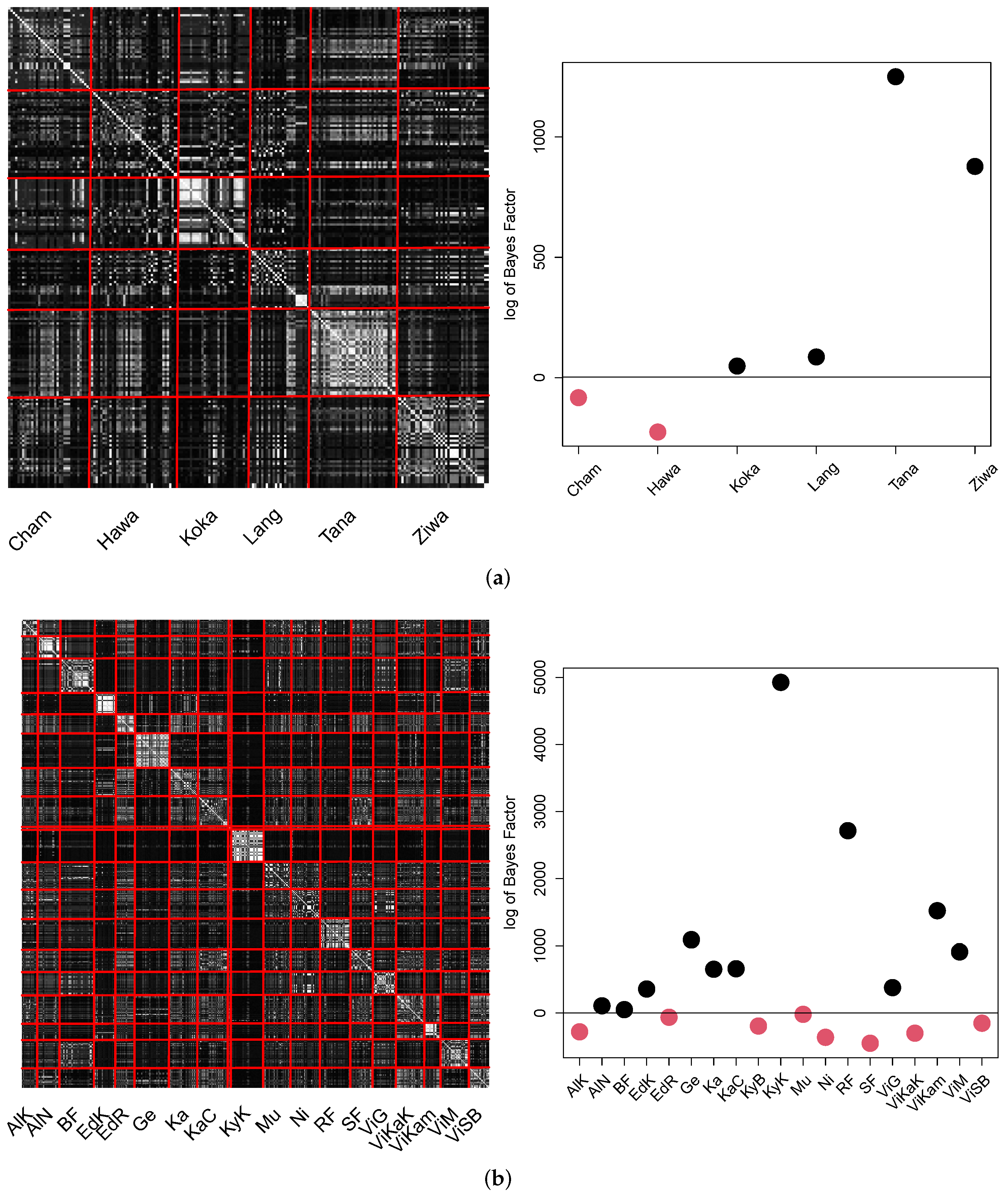
3.4. Latent Structure Investigation Relying on pCA
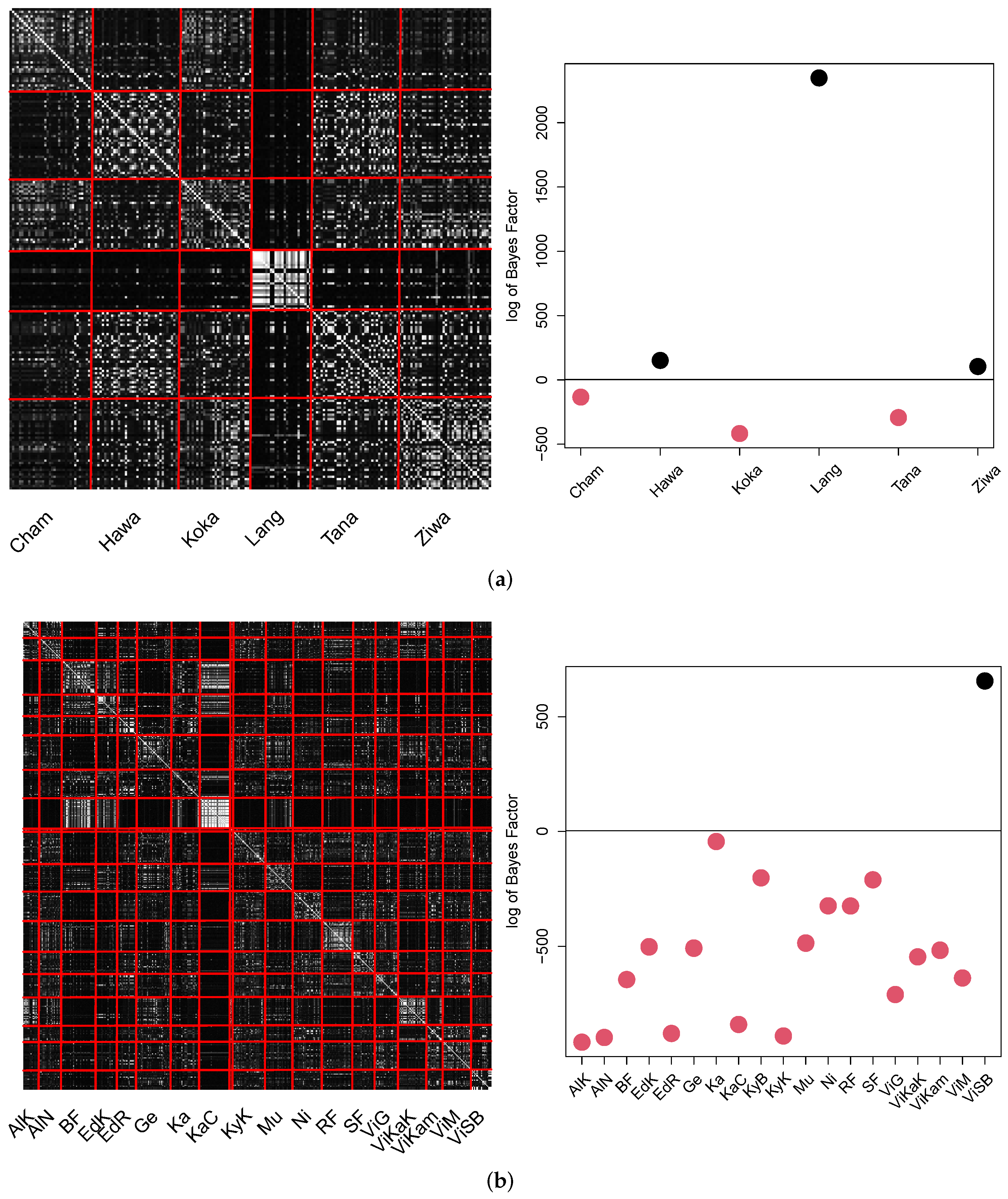
The pCA result for GPA for both datasets is summarized in in the pCA matrix as well as the Bayes factor plot in
Figure 13.
The results show that minor individual population location structure was identified to be different. Three out of six locations in Ethiopia (Hawassa, Langano and Ziway) and one out of nineteen locations in Uganda (Victoria Sango Bay) were identified to be significantly different. We emphasize that the pCA matrix visualization may lead to incomprehensible results in the Bayes factor analysis due to the brightness. The Bayes factor investigation is based on the comparison of the intra-location similarity. Thus this value decreases, even if minor obvious relations were measured in the remaining locations.
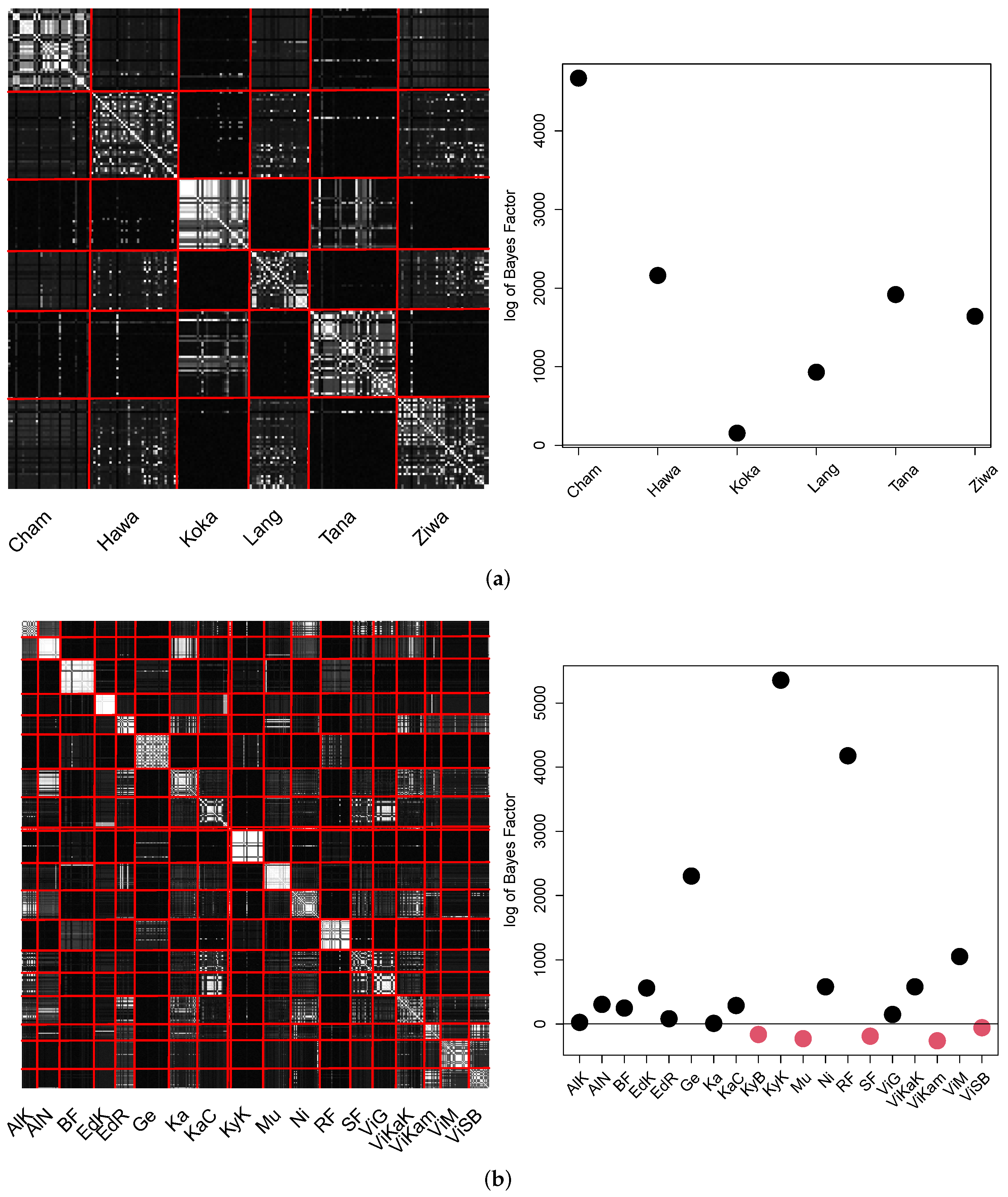
The results obtained by the B-GP-LVM are visualized in
Figure 14.
The pCA matrix for Ethiopia appears to be noisy. However, the individual probability values of the intra population locations exceed the probability values of inter population locations. This led to four out of six populations in Ethiopia which were significantly different to the other populations. Different to the GPA, lake Tana appears to be significantly different to the remaining locations. This significant difference and distinctiveness of the Lake Tana population has also been reported at molecular genetic level [
28,
29]. The pCA matrix for Uganda shows visible structure for the individual locations. The different locations in the same water bodies (e.g., the lake Victoria locations) are visible. However, similarities of these water bodies (e.g., Albert or Victoria) are visible as well. Eleven out of nineteen of Uganda’s population locations significantly differed from the remaining locations.
Finally, the results for cAE are summarized in the visualizations in the
Figure 15.
In both pCA matrices, the majority of locations can be clearly distinguished. All locations of Ethiopia were found to be significantly different to the remaining locations. Fourteen of nineteen locations in Uganda differed significantly. However, again the locations of Lake Viktoria did show similarities.
We summarize our findings of the proposed approach in
Table 3, where the population’s locations (which were observed to be significantly different) are marked with a cross (×).
We observed that for all applied methods the locations Langano and Ziway significantly differed from the remaining populations in Ethiopia. Furthermore, the location Victoria Sango Bay in Uganda was observed to be significantly different, only relying on GPA scaled landmarks. The locations Kyoga Bukungu, Mulehe Musezero as well as the Sindi Farm in Uganda were never observed to be significantly different to the remaining locations.
4. Discussion
This study investigated the quality of extracted GPA scaled coordinates in contrast to machine learning-based features. The quality was measured by the differentiability of the known population locations. To obtain comparable latent structures, the consensus clustering method was extended by a probabilistic interpretation as well as a hypothesis test.
Manually placed landmarks were extracted from image datasets obtained in Ethiopia and Uganda. These landmarks were processed using GPA. The results were statistically investigated. We observed significant relation of the GPA scaled coordinates to the population locations. Furthermore, a significant relation of the locations to the Procrustes distance was obtained. Relying on the visualization of the GPA coordinates (see
Figure 6), as well as the Spearman’s rank correlation tests, we concluded that the landmark-based approach results in a interpretable reduction of the image data with significant correlation to the populations location. Nevertheless, the GPA-scaled coordinate visualizations and hypotheses tests do not quantify the discriminability of the populations unveiled by the GPA approach. Furthermorer, the multivariate analysis showed overlapping population distribution in the PCA and ICA reduced GPA coordinates.
The proposed pCA was able to unveil significant differences for three out of six locations in Ethiopia. One of nineteen locations was found to be significantly different from the other locations in Uganda. Ref. [
24] obtained similar results for supervised Nile tilapia location classification using biologically interpretable GP-LVM features as well as GPA-scaled coordinates. Their results, enhanced by the latent structure investigation of this study show, that classic landmark based-approaches are limited in terms of information discovery. Regardless, the landmark-based approaches outperform the autonomous deep learning counterparts in terms of biological explainability. The machine learning-based approaches were investigated with visualization methods and major focus on biological uninformative image regions was removed.
In contrast to the manually placed landmarks of the GPA, the GP-LVM learns a latent representation of the specimen images. After training, the model reproduces the image content including background information such as specimen mounting material. We manually removed uninformative biological features using the variance-based feature visualization technique. The automation of this procedure is still an open problem in machine learning [
69].
The features which were visualized and shown to focus on biological meaningful information were in similar specimen locations to the GPA results. These features were tested using Spearman’s rank correlation test. This test indicates a significant relation of the chosen features to the population’s locations. Similar to the GPA-scaled landmarks, the multivariate analysis showed overlapping population location distributions. However, the pCA method was able to obtain population structures significantly different to other locations. Four of six locations of Ethiopia were shown to be significantly different. Eleven out of nineteen locations in Uganda were shown to be significantly different. This already shows an improvement compared with previous analyses based on classical morphometrics, where just a few populations were clearly separated [
5]. However, the GP-LVM still has limitations. The GP-LVM learns the latent representation of the image datasets using a set of Gaussian processes. On the one hand, the learning procedure is limited in terms of statistical black-box modeling [
31]. Furthermore the optimization procedure does not include biological knowledge. The learning procedure could be enhanced using prior biological knowledge in the variational approximation of the model [
46].
Similar to the GP-LVM, the cAE learns a latent representation using a learning procedure. Instead of a set of Gaussian processes, the cAE relies on an architecture of artificial neurons including convolutional layers. The latent features were processed in the same manner as GP-LVM features, including manual feature selection focusing on biologically meaningful image regions. All locations in Ethiopia and fourteen of the nineteen locations in Uganda were obtained to be significantly different relying on the pCA. However, the visualization of the selected features show noisy image regions. The reasons for this noisy visualization may be related to the dependent feature space learned by the cAE. The independent variation procedure for visualization may not be applicable for the learned feature space. Furthermore, the limitations of the GP-LVM are the same for the cAE.
We conclude this section by emphasizing the biological explainability of the manually placed landmarks. However, minor population location differences were obtained relying on GPA-scaled coordinates. The machine learning-based methods resulted in major population location differences relying on the pCA. We emphasize that the machine learning models were trained without knowledge of the known population clusters.
Thus, we fail to reject both hypotheses of this study and conclude that the machine learning models can learn biological meaningful features and that these features have a higher relation to the true population clusters than landmark-based features. We conclude that these features do contain information useful for population location discriminability and that the machine learning features exceed the explanation power of the used landmark-based method. Furthermore, our results indicates that larger parts of the specimens (e.g., the head in its entirety or the caudal fin region) are related to population locations. The visualizations of the learned features show that the machine learning models focus on areas with no landmarks. We recommend the investigation of these areas using GPA with additional landmarks. Furthermore, we recommend the GP-LVM for further investigation, including the integration of biological knowledge in the model as well as additional explanation investigation of the deep convolutional autoencoder due to the results of the pCA.
5. Summary
This study unveiled the explanatory power of image processing methodologies for visible diversity investigation. Generalized Procrustes analysis was compared to Gaussian process latent variable models as well as a convolutional autoencoder. Relying on two image databases, GPA-scaled coordinates as well as GP-LVM- and cAE-based features were extracted. The biological explanatory power of all applied methods was investigated. Furthermore, Spearman’s rank correlation test was used to investigate the relation of the obtained features to the population’s locations. However, a multivariate analysis of the aforementioned features showed that the population distributions overlaps. In order to overcome this problem and unveil the latent structure available in the image representations, a probabilistic consensus analysis was proposed.
Relying on the pCA, several GMMs were combined and the overall latent structure was visualized using the pCA matrix. Based on the model consensus, a Bayesian hypothesis test was formulated. The machine learning models outperformed the landmark based method. However, restricted explainability limits the biological usage of these models. The GP-LVM resulted in explainable image regions. Regardless, the behavior of the model is not fully explained. On the other hand, the performance of the cAE relies on very noisy image regions. However, the visualization technique used was discussed to be limited for cAE applications and the explanatory factors for the cAE may be still hidden in the model.
We conclude this study by emphasizing the performance of the machine learning models in terms of unsupervised features extraction. We recommend further research to investigate the explanatory methodologies in order to fully unveil the explanatory factors of the models. Furthermore, we recommend including existing biological knowledge in order to convert the black box models to fully explainable statistical tools.


 ,
, 


