Multi-Objective Optimization of Drilling Trajectory Considering Buckling Risk

Abstract

Directional drilling involves three sections—vertical, curved, and horizontal—and is used for drilling offshore wells and mining unconventional resources. The initial design of a well trajectory is important because the total length of the well trajectory is associated with the drilling cost; furthermore, the drag force and torque may cause buckling and damage the drill pipe. The well trajectory should be optimized considering the length and load of drill pipes. In this study, a new method of optimizing directional well trajectory is used to formulate the objective function considering the length, drag, and torque. To verify the applicability of this method, we applied it to an actual oil well and a theoretical oil well. The results obtained show that the use of the proposed method in the initial design of drilling trajectory can reduce the torque by up to 15%, drag by 2.6%, and length by 8.5% for the two models used in this study. This method is safer as it reduces the risk of buckling compared to the design that relies on the previous designer’s experience, and it reduces the trajectory length; thus, it can save time and costs of drilling.

1. Introduction

Unlike vertical drilling, which is the conventional drilling method, in directional drilling, drilling is intentionally performed through a non-vertical path to reach an underground target point. This drilling method is widely used to reach a target layer in underground areas where vertical drilling cannot be performed owing to environmental factors such as densely populated areas, mountains, lakes, or environmentally sensitive areas. In the case of offshore oil fields, it is possible to create multiple boreholes on one platform, and they can be closed and drilled in another direction if problems occur during drilling. Because drilling offshore oil fields is more expensive than drilling onshore oil fields, directional drilling methods are more cost-effective than vertical drilling. Figure 1 shows various applications of directional drilling.

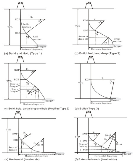
Figure 1. Several applications of directional drilling. Adapted with permission from Ref. [1]. 2014 Kim et al.

Figure 2 shows that directional drilling can be divided into five types according to the section: hold section, build-up section, drop off section, side bend section, and horizontal section. The hold section is a straight section; the build-up section, drop off section, and side bend section are curved; and the horizontal section is planar.

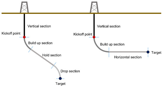
Figure 2. Trajectory section of directional drilling.

If the kickoff point (KOP), which is the point where a vertically running directional pipe exhibits directional properties for the first time, becomes closer to the target point, the drilling trajectory will produce a large angle change within a short section, resulting in excessive torque and drag [2]. Excessive torque and drag can create doglegs, which are sudden changes in a direction that appear like a dog’s hind legs, and key seating, in which grooves are formed in the wall of the borehole by drill collars or other tools in the borehole. In addition, if the drilling tools and casing are damaged, it can lead to a huge increase in drilling costs [3]. Therefore, it is critical to select appropriate KOPs to reduce the distributed load in the drilling trajectory [4]. Furthermore, directional drilling is more significantly affected by the buckling effect than vertical drilling. The buckling effect is a type of deformation of the drilling tube in which the drilling pipe is twisted or bent owing to its weight, frictional force in the borehole, and torque from the rotation of the drill bit. The deflection of the drilling pipe becomes more severe owing to the buckling effect, and this can cause the lock-up phenomenon, which prevents the drilling pipe from moving [5]. Furthermore, the buckling effect can interfere with the control of the drilling direction and effective load transfer within the drilling pipe, causing delays in the drilling time and increasing the drilling cost [6]. Therefore, in this study, we performed optimization to select the shortest path when designing the drilling trajectory considering the risk of buckling. Furthermore, as these problems have multiple objective functions, multi-objective optimization is required [7]. This approach reduces the drilling time as well as the cost.

To resolve the problems caused by buckling of the pipe, Aadnøy [8] focused on calculation of the load in the directional drilling trajectory and proposed an analytical model. Ismayilov [9] analyzed an actual oil well by comparing the results obtained from an analytical model proposed by Aadnøy [8] for calculating the friction of the well, a commercial program, and the actual drag and torque measurements. In addition, in a study on the buckling of directional drilling for oil wells, Wu and Juvkam-Wold [5] proposed a model for buckling loads.

Many researchers have attempted to use multi-objective optimization in relation to drilling pipes [10,11,12]. Shokir et al. [13] studied the length of the drilling trajectory, which is related to drilling costs. Optimization was performed for the length of the three-dimensional trajectory using a genetic algorithm.

In this paper, we present an optimization method that minimizes the risk of buckling and the total length of the drilling trajectory by minimizing the drag and torque, which are the loads on the drilling pipe. To this end, the objective function is defined in terms of the total length of the drilling trajectory and the load acting on the drilling pipe, and the design variables include the azimuth, inclination, dogleg severity, and kickoff point. In addition, the particle swarm optimization (PSO) algorithm is used for optimization. The PSO algorithm is suitable for multi-objective optimization related to buckling [14,15]. To verify the method proposed in this paper, it was compared with earlier results of the optimization of the drilling trajectory, including the total length of the drilling trajectory, load acting on the drilling pipe, and occurrence of buckling.

If the orbit is designed according to the method presented in this paper, the length of the drilling orbit can be reduced to save time and money consumed in drilling. In addition, the risk related to buckling can be reduced, improving the drilling safety.

2. Definition of Target System

A typical directional drilling trajectory, which is the main topic of this study, is shown in Figure 3, and Table 1 presents the nomenclature for the calculation of the length of the drilling trajectory.

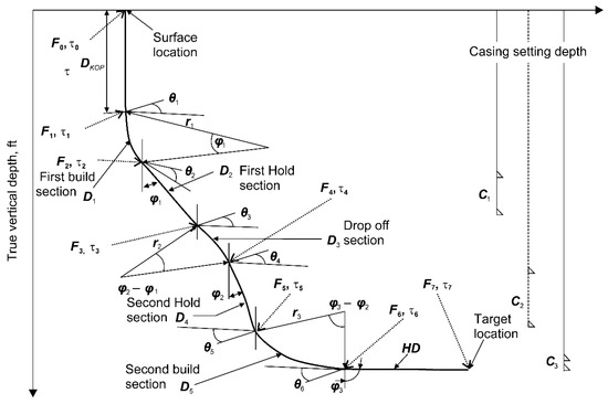
Figure 3. Vertical plan of a general 3D horizontal well trajectory. Adapted with permission from Ref. [13]. 2004 Shokir, E.E.M. et al.

Table 1. Nomenclature of variables used to calculate the length of the drilling trajectory.

Symbol	Definition
${\phi }_1$	First hold angles (°)
${\phi }_2$	Second hold angles (°)
${\phi }_3$	Third hold angles (°)
${\theta }_1$	Azimuth angle at the kickoff point (°)
${\theta }_2$	Azimuth angle at the end of the first build section (°)
${\theta }_3$	Azimuth angle at the end of the first hold section (°)
${\theta }_4$	Azimuth angle at the end of the drop section (°)
${\theta }_5$	Azimuth angle at the end of the second hold section (°)
${\theta }_6$	Azimuth angle at the end of the second build section (°)
$T_1$	Dogleg severity of the first build section (°/100 ft)
$T_2$	Dogleg severity of the first hold section (°/100 ft)
$T_3$	Dogleg severity of the drop section (°/100 ft)
$T_4$	Dogleg severity of the second hold section (°/100 ft)
$T_5$	Dogleg severity of the second build section (°/100 ft)
$TMD$	True measured depth of the well (ft)
$TVD$	True vertical depth of the well (ft)
$D_{KOP}$	True vertical depth of the kickoff point (ft)
$D_{v2}$	True vertical depth at the end of the first hold section (ft)
$D_{v3}$	True vertical depth at the end of the drop section (ft)
$r$	Radius of curvature (ft)
$D$	Length of the segment (ft)
$HD$	Horizontal section (ft)
$a$	Curvature of the curve (rad/ft)
$C$	Casing setting depth (ft)

In this study, we used information on an actual oil well A, which is located in the Gulf of Suez, Egypt, and information on a theoretical oil well B for the analysis.

Table 2 presents data on the drilling trajectories for wells A and B designed using the conventional method. The definitions of the symbols in the figure are given in Table 1.

Table 2. Well data for the applications.

	Application A (Actual Well)	Application B (Theoretical Well)
True measured depth (ft)	15,565	13,000
Casing setting depth after 1st build (ft)	Neglect	Neglect
Casing setting depth after 2nd build (ft)	Neglect	Neglect
Casing setting depth after 3rd build (ft)	Neglect	Neglect
$TVD$ (ft)	10,848	9410.7
Target North–South (ft)	6284	1984.6
Target East–West (ft)	−3.252	3975.4
$D_{KOP}$ (ft)	625	1000
Depth of 2nd build point (ft)	6600	5000
Depth of 3rd build point (ft)	11,260	10,000
${\phi }_1$ (°)	15	20
${\phi }_2$ (°)	45	40
${\phi }_3$ (°)	90	90
${\theta }_1,$${\theta }_2$$, {\theta }_3$$, {\theta }_4$$, {\theta }_5$$, {\theta }_6$ (°)	-	-
$T_1$$(°/100$ ft)	0.9	1.0
$T_2$$(°/100$ ft)	0.0	0.0
$T_3$$(°/100$ ft)	2	1.0
$T_4$$(°/100$ ft)	0.0	0.0
$T_5$$(°/100$ ft)	3.5	3.5

3. Formulation of Directional Drilling Trajectory Problem

3.1. Definition of Objective Function for Optimization

3.1.1. Length of Oil Well

Many methods have been used to calculate the length of the drilling trajectory. In the design of the horizontal well, the length of a three-dimensional drilling trajectory with an azimuth angle ($\theta$), inclination angle ($\phi$), and radius of curvature ($r$) is the length between two points in space, as shown in Figure 4, and can be calculated using Equation (1) [16].

$$\Delta MD=r\sqrt{{\left({\theta }_2-{\theta }_1\right)}^2{\sin }^4\left(\frac{{\phi }_1-{\phi }_2}{2}\right)+{\left({\phi }_2-{\phi }_1\right)}^2} .$$

(1)

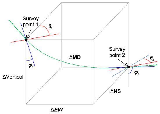
Figure 4. Surveys’ calculation variables.

In Equation (1), the radius of curvature ($r$) can be calculated as given in Equation (2), where $T$ is the dogleg severity (Table 2); this is the angle rate at which the drilling trajectory changes per 100 ft.

$$r=\frac{180}{\pi }\times \frac{100}{T}.$$

(2)

The length of the drilling trajectory can be calculated from Equations (1) and (2) by changing the azimuth angle and the radius of curvature of the drilling trajectory between two points.

In addition, the north–south distance between two points can be calculated using Equation (3), the east–west distance using Equation (4), and the vertical distance using Equation (5) [17].

$$\Delta NS=\frac{\Delta MD\left(\cos \left({\phi }_1\right)-\cos \left({\phi }_2\right)\times \left(\sin ({\theta }_2\right)-\sin \left({\theta }_1\right)\right)}{\left({\phi }_2-{\phi }_1\right)\times \left({\theta }_2-{\theta }_1\right)}$$

(3)

$$\Delta EW=\frac{\Delta MD\left(\cos \left({\phi }_1\right)-\cos \left({\phi }_2\right)\times \left(\cos ({\theta }_1\right)-\cos \left({\theta }_2\right)\right)}{\left({\phi }_2-{\phi }_1\right)\times \left({\theta }_2-{\theta }_1\right)}$$

(4)

$$\Delta Vertical=\frac{\Delta MD\left(\sin \left({\phi }_2\right)-\sin \left({\phi }_1\right)\right)}{\left({\phi }_2-{\phi }_1\right)}.$$

(5)

The directional drilling trajectory shown in Figure 3 can be divided into sections: the kickoff section ($D_{KOP}$), the build-up and drop off sections ($D_1, D_3, D_5$), the hold sections ($D_2, D_4$), and the horizontal section ($HD$). If all the sections are summed up, the total measured depth ($TMD$) can be calculated, where ${\phi }_{KOP}$ is the inclination angle at the kickoff section and is assumed to be 0°. The relevant equations are Equations (6)–(11).

$$TMD=D_{KOP}+D_1+D_2+D_3+D_4+D_5+HD$$

(6)

$$D_1=r_1\sqrt{{\left({\theta }_2-{\theta }_1\right)}^2{\sin }^4\left(\frac{{\phi }_1+{\phi }_{KOP}}{2}\right)+{\left({\phi }_1-{\phi }_{KOP}\right)}^2}$$

(7)

$$D_2=\frac{\left(D_{v2}-D_{KOP}-D_1\right)\times \left(\sin \left({\phi }_1\right)-\sin \left({\phi }_{KOP}\right)\right)}{{\phi }_1-{\phi }_{KOP}}$$

(8)

$$D_3=r_3\sqrt{{\left({\theta }_4-{\theta }_3\right)}^2{\sin }^4\left(\frac{{\phi }_2+{\phi }_1}{2}\right)+{\left({\phi }_2-{\phi }_1\right)}^2}$$

(9)

$$D_4=\frac{(D_{v3}-D_{v2}-D_3)\times (\sin \left({\phi }_3\right)-\sin \left({\phi }_2\right))}{{\phi }_2-{\phi }_1}$$

(10)

$$D_5=r_5\sqrt{{\left({\theta }_6-{\theta }_5\right)}^2{\sin }^4\left(\frac{{\phi }_3+{\phi }_2}{2}\right)+{\left({\phi }_3-{\phi }_2\right)}^2}.$$

(11)

The radius of curvature in each section is calculated as given in Equation (12).

$$r_i=\frac{18000}{\pi \times T_i}, i=1 ~ 5.$$

(12)

The casing depth in each section is calculated using Equations (13)–(15).

$$C_1=D_{KOP}+D_1\times \frac{\sin \left({\phi }_1\right)}{{\phi }_1}$$

(13)

$$C_2=D_{KOP}+D_1\times \frac{\sin \left({\phi }_1\right)}{{\phi }_1}+D_2\times \cos \left({\phi }_1\right)+D_3\times \frac{\sin \left({\phi }_2\right)-\sin \left({\phi }_1\right)}{{\phi }_2-{\phi }_1}$$

(14)

$$\begin{array}{cc}\hfill C_3=D_{KOP}+D_1& \times \frac{\sin \left({\phi }_1\right)}{{\phi }_1}+D_2\times \cos \left({\phi }_1\right)+D_3\times \frac{\sin \left({\phi }_2\right)-\sin \left({\phi }_1\right)}{{\phi }_2-{\phi }_1}+D_4\hfill \\ & \times \cos \left({\phi }_2\right)+D_5\times \frac{\sin \left({\phi }_3\right)-\sin \left({\phi }_2\right)}{{\phi }_3-{\phi }_2}. \hfill \end{array}$$

(15)

The dogleg angle is the angle of each section, and this can be calculated using Equations (16)–(20).

$$D{L}_{A1}=T_1\times \frac{D_1}{100}, \mathrm{where} D{L}_{A1}={\phi }_1$$

(16)

$$D{L}_{A2}=T_2\times \frac{D_2}{100}, \mathrm{where} D{L}_{A2}\cong 0$$

(17)

$$D{L}_{A3}=T_3\times \frac{D_3}{100}, \mathrm{where} D{L}_{A3}={\phi }_2-{\phi }_1$$

(18)

$$D{L}_{A4}=T_4\times \frac{D_4}{100}, \mathrm{where} D{L}_{A4}\cong 0$$

(19)

$$D{L}_{A5}=T_5\times \frac{D_5}{100}, \mathrm{where} D{L}_{A5}={\phi }_3-{\phi }_2.$$

(20)

3.1.2. Drag and Torque

Drag is generated by friction between the drilling pipe, borehole wall, and drilling mud during the tripping process in which the drilling pipe is raised or lowered, and torque is generated by the rotation of the bit during drilling. To calculate the load on the pipe in various drilling trajectories, Aadnøy [8] proposed the following method, in which it is assumed that the bending stiffness of the drilling pipe is negligibly small, and the trajectory is classified into a straight trajectory and a random trajectory.

First, the drag induced in the hold section, which is an inclined straight line, is proportional to the weight of the drilling pipe, as shown in Figure 5, and the force at the top can be calculated using Equation (21).

$$F_2=F_1+\beta w\Delta L\left(\cos \phi \pm \mu \sin \phi \right)$$

(21)

where $F_2$ is the force at the top of the section, $F_1$ is the force at the bottom of the section, $\beta$ is the buoyancy constant, $w$ is the weight per unit length of the drilling pipe, $\Delta L$ is the length of the section, $\phi$ is the angle of inclination of the section, $\mu$ is the friction coefficient, and the ± in the second term indicates upward and downward of the drilling pipe, respectively.

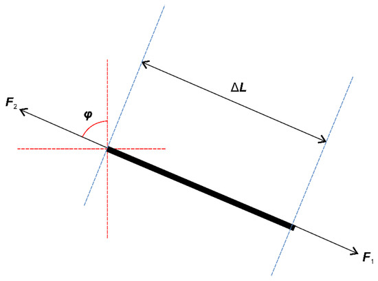
Figure 5. Load of the hold section.

The torque ($\tau$) in the hold section is calculated by multiplying the friction coefficient by the radius of the pipe joint tool as given in Equation (22), where $R$ is the radius of the pipe joint tool.

$$\tau =\mu R\beta w\Delta L\sin \phi .$$

(22)

The drag in the curved section shown in Figure 6 is the contact force between the borehole and drilling pipe and is significantly affected by the axial load. As a result, this drag is related to tension. For example, the tension acting on a short pipe can be greater than the internal bending load. In addition, the dogleg angle depends on both the inclination angle and the azimuth angle, and the axial force for the drop off section, build-up section, side bend section, or a combination of these sections is calculated using Equation (23).

$$F_2=F_1{e}^{\pm \mu \left|D{L}_{A2}-D{L}_{A1}\right|}+\beta w\Delta L\left(\frac{\sin {\phi }_2-\sin {\phi }_1}{{\phi }_2-{\phi }_1}\right).$$

(23)

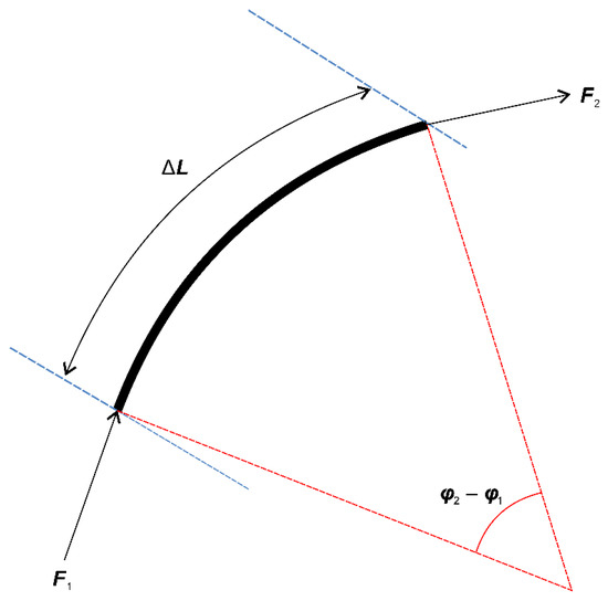
Figure 6. Load of the curve section.

The torque for the curve section is given by Equation (24).

$$\tau =\mu RN=\mu R{F}_1\left|D{L}_{A2}-D{L}_{A1}\right|.$$

(24)

Equations (21)–(24) can be solved for any drilling trajectory shape by dividing it into straight and curved elements, and the drag and torque are calculated from the end of the drilling trajectory.

Because the drag and torque act on the drilling pipe simultaneously, Equation (25) can be used to calculate the magnitude of the load in each section.

$$P_i=\sqrt{F_i^2+{\left(\frac{{\tau }_i}{r_p}\right)}^2}$$

(25)

where $P_i$ represents the ultimate load on the drilling pipe in any section and $r_p$ is the radius of the drilling pipe.

The load on the drilling pipe in a random section can be calculated using the above equation based on the shape of the section after determining the load at the lowest point.

In the method proposed by Aadnøy [8], the temperature change and the suspended particles in each section are not considered because the friction coefficients in the entire section of the drilling trajectory are calculated using the average value. It is necessary to use the cutting transport theory if the friction coefficient needs to be applied to each section for accurate calculation as it does not reflect regional characteristics [9,18].

3.1.3. Buckling of Drilling Pipe

Buckling refers to a phenomenon in which a drilling pipe is bent or twisted owing to an increase in the load applied to it. Buckling load represents the smallest amount of load in which buckling can occur. It is determined according to the weight and property of the drilling pipe and the shape of the drilling trajectory section. The buckling load can be divided into the critical buckling load ($F_{cr}$) and helical buckling load ($F_{hel}$). It can be compared with loads such as drag and torque distributed at the point of the drilling trajectory section to determine whether sinusoidal buckling and helical buckling occur.

Sinusoidal buckling and helical buckling are defined according to the degree of bending of the drilling pipe. Sinusoidal buckling is the bending of the initial borehole, as shown in Figure 7. The borehole has the shape of a sinusoidal wave. If the load continues to increase, the pipe becomes severely bent or twisted in a spiral form and comes into contact with the borehole wall, resulting in helical buckling, as shown in Figure 8. Sinusoidal buckling does not have a significant effect on drilling operations, but helical buckling makes it difficult to control the direction of the drilling pipe and impedes the effective transmission of the load to the drilling pipe. If the degree of deflection is more severe, the drilling pipe can no longer be moved regardless of the amount of load applied, or a lock-up will occur. Directional drilling, such as horizontal drilling, is a risk factor that must be avoided owing to the high level of damage, including delays in drilling work and increased costs from helical buckling.

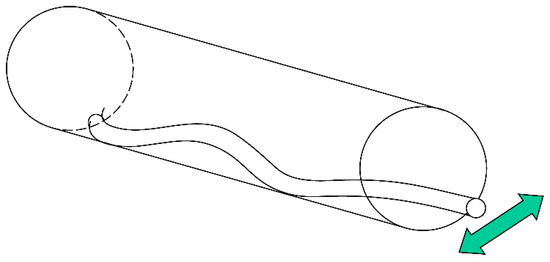
Figure 7. Sinusoidal buckling.

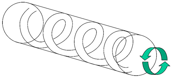
Figure 8. Helical buckling.

The buckling load model applied in this study can be divided into critical buckling load and helical buckling load based on the shape of the drilling trajectory section, as presented in Table 3 and Table 4 [5].

Table 3. Critical buckling load for various sections.

	Critical Buckling Load (lbf)
Horizontal wellbore	$F_{cr}=2\sqrt{\frac{EI{W}_e}{d}}$
Inclined wellbore	$F_{cr}=2\sqrt{\frac{EI{W}_e\sin \phi }{d}}$
Vertical wellbore	$F_{cr}=2.55\sqrt[3]{EI{W}_e^2}$
Build wellbore	$F_{cr}=\frac{4EI}{rd}\left(1+\sqrt{1+\frac{d{r}^2{W}_e\sin \phi }{4EI}}\right)$

Table 4. Helical buckling load for various sections.

	Helical Buckling Load (lbf)
Horizontal wellbore	$F_{hel}=2\left(2\sqrt{2}-1\right)\sqrt{\frac{EI{W}_e}{d}}$
Inclined wellbore	$F_{hel}=2\left(2\sqrt{2}-1\right)\sqrt{\frac{EI{W}_e\sin \phi }{d}}$
Vertical wellbore	$F_{hel}=5.55\sqrt[3]{EI{W}_e^2}$
Build wellbore	$F_{hel}=\frac{12EI}{rd}\left(1+\sqrt{1+\frac{R{r}^2{W}_e\sin \phi }{8EI}}\right)$

In Table 3 and Table 4, $E$ is the Young’s modulus, $I$ is the moment of inertia, $r$ is the radius of curvature of the drilling trajectory, $d$ is the spatial distance between the bore and the wall of the borehole, $\phi$ is the inclination angle, and $W_e$ is the effective weight of the borehole within the drilling trajectory [6].

3.1.4. Objective Function Definition

For the objective function, it is necessary to minimize the length of the drilling trajectory and the load on the drilling pipe. For this purpose, the minimum length model of the drilling trajectory can be a model that minimizes Equation (6), which can be employed to calculate the total length of the drilling trajectory as given in Equation (26).

$$\mathrm{Minimize} f_1\left(x\right)=TMD.$$

(26)

The load induced on the drilling pipe can be divided into drag and torque. This load can be defined as below. First, the drag of each section can be calculated by dividing the trajectory into a straight section and a curved section based on Equations (21) and (23), and these are expressed in Equations (27)–(33).

$$F_6=F_7+\beta wHD\left(\cos {\phi }_3+\mu \sin {\phi }_3\right)$$

(27)

$$F_5=F_6{e}^{\mu \left|D{L}_{A5}-D{L}_{A3}\right|}+\beta w{D}_5\left(\frac{\sin {\phi }_3-\sin {\phi }_2}{{\phi }_3-{\phi }_2}\right)$$

(28)

$$F_4=F_5+\beta w{D}_4\left({\cos \mathsf{\phi }}_2+\mu \sin {\phi }_2\right)$$

(29)

$$F_3=F_4{e}^{\mu \left|D{L}_{A3}-D{L}_{A1}\right|}+\beta w{D}_3\left(\frac{\sin {\phi }_2-\sin {\phi }_1}{{\phi }_2-{\phi }_1}\right)$$

(30)

$$F_2=F_3+\beta w{D}_2\left(\cos {\phi }_1+\mu \sin {\phi }_1\right)$$

(31)

$$F_1=F_2{e}^{\mu \left|D{L}_{A3}-D{L}_{A1}\right|}+\beta w{D}_1\left(\frac{\sin {\phi }_1-\sin {\phi }_{KOP}}{{\phi }_1-{\phi }_{KOP}}\right)$$

(32)

$$F_0=F_1+\beta w{D}_{KOP}\left(\cos {\phi }_{KOP}+\mu \sin {\phi }_{KOP}\right).$$

(33)

The torque in each section can be calculated by dividing it into a straight section and a curved section based on Equations (22) and (24); these are given in Equations (34)–(40).

$${\tau }_6=\mu R\beta wHD\sin {\phi }_3$$

(34)

$${\tau }_5=\mu R{F}_6\left|D{L}_{A5}-D{L}_{A3}\right|$$

(35)

$${\tau }_4=\mu R\beta w{D}_4\sin {\phi }_2$$

(36)

$${\tau }_3=\mu R{F}_4\left|D{L}_{A3}-D{L}_{A1}\right|$$

(37)

$${\tau }_2=\mu R\beta w{D}_2\sin {\phi }_1$$

(38)

$${\tau }_1=\mu R{F}_2\left|D{L}_{A1}\right|$$

(39)

$${\tau }_0=\mu R\beta w{D}_{KOP}\sin {\phi }_{KOP}.$$

(40)

In each section, the occurrence of sinusoidal buckling or helical buckling was confirmed using Table 3, Table 4 and Table 5. If the total sum of the final loads in all sections (P) is minimized, then the load on the entire drilling trajectory can be minimized. Therefore, the objective function can be defined as given in Equation (41).

$$\mathrm{Minimize} f_2\left(x\right)={{\displaystyle \sum }}^{ }{P}_{i.}$$

(41)

Table 5. Drill pipe behaviors according to load condition.

Load Condition	Drill Pipe Behaviors
$F<F_{cr}$	No buckling
$F_{cr}\le F<F_{hel}$	Sinusoidal buckling
$F_{hel}\le F$	Helical buckling

The objective function can be defined by multiplying the length minimization model and the load minimization model by the weight of the drilling trajectory, as given in Equation (42).

$$\mathrm{Minimize} f\left(x\right)=W_1\times \left(\frac{f_1\left(x\right)}{f_{1i}\left(x\right)}\right)+W_2\times \left(\frac{f_2\left(x\right)}{f_{2i}\left(x\right)}\right)$$

(42)

where $f_{1i}\left(x\right)$ and $f_{2i}\left(x\right)$ are the initial values of each term and are used for the normalization of each term. $W_1$ and $W_2$ are the weights of each term, and the sum of the weights should be one. By adjusting the weight in the objective function, the designer can design the drilling track trajectory by giving more weight to the length of the drilling trajectory or the load on the drilling pipe (see Section 4.1).

In addition to the design variables, the values required to evaluate the objective function are listed in Table 6, and these values are equally applied to wells A and B.

Table 6. Setting of the fixed value.

	Value
$\mathrm{Friction} \mathrm{factor} \left(\mu \right)$	0.15
$\mathrm{Drill} \mathrm{pipe} \mathrm{weight} \left(w\right)$ (lbf/ft)	6.65
Drill pipe ID (in)	1.815
Drill pipe OD (in)	2 3/8
$\mathrm{Buoyancy} \mathrm{factor} \left(\beta \right)$	0.8
Tool joint OD (in)	3 3/8
$\mathrm{Modulus} \mathrm{of} \mathrm{elasticity} \left(E\right)$ (psi)	3 × 107

3.2. Definitions of Constraints for Optimization

The constraints for the design variables in this study are listed in Table 7. For the constraints, a pre-survey can be conducted to establish points to be avoided in the design of the drilling trajectory owing to environmental and geological factors. In this study, the constraints used in [13] were used.

Table 7. Constraints used in this research. Adapted with permission from Ref. [13]. 2004 Shokir, E.E.M. et al.

	Application A (Actual Well)	Application B (Theoretical Well)
True vertical depth (ft)	$\mathrm{10,850}\le TVD\le \mathrm{10,900}$	$9385\le TVD\le 9435$
$\mathrm{Inclination} \mathrm{angle} (°)$	$10\le {\phi }_1\le 20$	$10\le {\phi }_1\le 30$
	$40\le {\phi }_2\le 70$	$30\le {\phi }_2\le 50$
	$90\le {\phi }_3\le 95$	$90\le {\phi }_3\le 95$
$\mathrm{Azimuth} \mathrm{angle} (°)$	$270\le {\theta }_1\le 280$	$300\le {\theta }_1\le 360$
	$270\le {\theta }_2\le 280$	$300\le {\theta }_2\le 360$
	$270\le {\theta }_3\le 280$	$300\le {\theta }_3\le 360$
	$330\le {\theta }_4\le 340$	$360\le {\theta }_4\le 460$
	$330\le {\theta }_5\le 340$	$360\le {\theta }_5\le 460$
	$355\le {\theta }_6\le 360$	$360\le {\theta }_6\le 460$
Dogleg severity $(°/100$ ft)	$T_1\le 5$	$T_1\le 5$
	$T_2\le 5$	$T_2\le 1$
	$T_3\le 5$	$T_3\le 5$
	$T_4\le 5$	$T_4\le 1$
	$T_5\le 5$	$T_5\le 10$
Depth of kickoff point (ft)	$600\le D_{KOP}\le 1000$	$500\le D_{KOP}\le 2000$
Depth of 2nd build point (ft)	$6000\le D_{v2}\le 7000$	$2000\le D_{v2}\le 7000$
Depth of 3rd build point (ft)	$\mathrm{10,000}\le D_{v3}\le \mathrm{10,200}$	$8000\le D_{v3}\le \mathrm{10,000}$
Casing setting depth after 1st build (ft)	$1800\le C_1\le 2200$	$1500\le C_1\le 4000$
Casing setting depth after 2nd build (ft)	$7200\le C_2\le 8700$	$7000\le C_2\le 9000$
Casing setting depth after 3rd build (ft)	$\mathrm{10,300}\le C_1\le \mathrm{11,000}$	$9000\le C_1\le \mathrm{10,000}$

4. Drilling Trajectory Optimization

4.1. Optimization Algorithm

Typical optimization algorithms using natural phenomena include the genetic algorithm (GA) and particle swarm optimization (PSO). Their common characteristics are that the objective function is used to solve a given problem, and that the optimal point is found simultaneously at several points based on the population. In addition, the entire solution field can be searched by examining any point [19]. However, the operator that operates the two algorithms and the part that controls convergence is different, and PSO is driven by fewer operators than GA. In addition, when the same code is repeatedly processed as in an optimization algorithm, convergence stagnation occurs. In the case of PSO, the optimal solution is effectively approached by adjusting the convergence by inertia weight. In the case of GA [20], this cannot be overcome, which is problematic. Therefore, in the case of GA, the number of operators that must be adjusted to obtain an optimal solution is large, and even a small change in the operator results in a large change, requiring the skill of the researcher. In this study, we tried to perform optimization using PSO, which is simple to implement and has a better convergence than that of GA [21]. Figure 9 shows a flowchart of the PSO algorithm.

Figure 9. Flowchart of the particle swarm optimization algorithm.

4.2. Optimization Process

Existing research results [13] were used to specify the initial values of the drilling trajectory length term of the objective function and the load term of the drilling pipe. The design variable values derived from the results obtained in existing research are summarized in Table 8 and were used in the objective function to confirm the initial length ($f_{1i}\left(x\right)$), initial load ($f_{2i}\left(x\right)$), and the occurrence of buckling for wells A and B.

Table 8. Design variables of the initial design. Adapted with permission from Ref. [13]. 2004 Shokir, E.E.M. et al.

	Application A	Application B
${\phi }_1$$(°)$	13.77	10.73
${\phi }_2$$(°)$	42.131	34.773
${\phi }_3$$(°)$	90	90
$T_1$$(°/100$ ft)	1.675	1.5195
$T_2$$(°/100$ ft)	0.047	0.00355
$T_3$$(°/100$ ft)	1.431	1.708
$T_4$$(°/100$ ft)	−0.0102	0.01258
$T_5$$(°/100$ ft)	2.413	1.9978
${\theta }_1$$(°)$	279.976	332.156
${\theta }_2$$(°)$	279.72	322.22
${\theta }_3$$(°)$	275.02	322.15
${\theta }_4$$(°)$	332.3	402.355
${\theta }_5$$(°)$	334.32	457.04
${\theta }_6$$(°)$	355	437.234
$D_{KOP}$ (ft)	987.975	934.2557
$D_{v2}$ (ft)	6801.37	6651.251
$D_{v3}$ (ft)	10,001.48	8090.88

Table 9 summarizes data for the total length and load of the drilling trajectories calculated by substituting the values in Table 8 for wells A and B. These data were used as the initial value for each term in the objective function.

Table 9. Calculation results of the initial design.

	Application A (Actual Well)	Application B (Theoretical Well)
$\mathrm{Total} \mathrm{measured} \mathrm{depth} \mathrm{of} \mathrm{the} \mathrm{initial} \mathrm{design}, f_{1i}\left(x\right)$ (ft)	15,127	12,829
$\mathrm{Total} \mathrm{load} \mathrm{of} \mathrm{the} \mathrm{initial} \mathrm{design}, f_{2i}\left(x\right)$ (lbf)	59,946	50,812

Using the values in Table 8, the occurrence of buckling in wells A and B was verified. The results are summarized in Table 10. The results indicate that helical buckling and sinusoidal buckling occurred.

Table 10. Verification of buckling of various sections.

	Application A	Application B
Horizontal section	No buckling	No buckling
Second build section	No buckling	No buckling
Second hold section	No buckling	No buckling
First drop section	Sinusoidal buckling	No buckling
First hold section	Helical buckling	Sinusoidal buckling
First build section	No buckling	No buckling

A formulation process was performed to define the objective function, design variables, and constraints based on the given drilling trajectory data, the length model, and the load model. Optimization was performed using MATLAB^® and the particle swarm optimization algorithm. The setting of the particle swarm optimization algorithm is presented in Table 11. The parametric setting values were optimized with various numerical values, and the value with the shortest calculation time and best result among those obtained was selected.

Table 11. Setting of the particle swarm optimization algorithm.

Parameter	Value
Maximum iteration	1000
Population size (swarm size)	1000
Inertia weight	0.9
C1	1.5
C2	2.0

5. Comparison of Optimization Results

Table 12 presents the values of the optimal design variables when the weights ($W_1, W_2$) that are multiplied by each term in the objective function are set to 0.5 during the optimization.

Table 12. Design variables of the optimization result.

	Application A	Application B
${\phi }_1$$(°)$	10	10
${\phi }_2$$(°)$	40	50
${\phi }_3$$(°)$	90	95
$T_1$$(°/100$ ft)	0.1657	0.1989
$T_2$$(°/100$ ft)	2.5443	0.3005
$T_3$$(°/100$ ft)	3.0187	3.3597
$T_4$$(°/100$ ft)	4.0363	0.5631
$T_5$$(°/100$ ft)	5	10
${\theta }_1$$(°)$	274.2409	318.9605
${\theta }_2$$(°)$	273.1937	307.9697
${\theta }_3$$(°)$	280	360
${\theta }_4$$(°)$	330	360
${\theta }_5$$(°)$	340	431.93
${\theta }_6$$(°)$	355	431.93
$D_{KOP}$ (ft)	1000	2000
$D_{v2}$ (ft)	7000	7000
$D_{v3}$ (ft)	10,000	8000

The optimization results, including the total length, load, and buckling of the drilling trajectories, were evaluated based on Table 12. The corresponding values are summarized in Table 13 and Table 14 by comparing them with the results in existing research (refer to Table 8). In the case of the load, it was divided into drag and torque after examining the occurrence of buckling. The drag that was applied to the entire borehole that constitutes the drilling trajectory is $F_0,$ and the torque was calculated using the following equation:

$${\tau }_{total}={\displaystyle \sum }_{i=0}^6{\tau }_i.$$

(43)

Table 13. Comparison of existing design and new design for application A.

Application A (Actual Well)
	Existing	New	New/Existing Ratio
Total measured depth (ft)	15,127	14,768	0.976
Total drag force (lbf)	62,567	61,116	0.976
Total torque (lbf.ft)	16,950	14,413	0.850
Horizontal section	No buckling	No buckling	-
Second build-up section	No buckling	No buckling	-
Second hold section	No buckling	No buckling	-
First drop off section	Sinusoidal buckling	No buckling	-
First hold up section	Helical buckling	No buckling	-
First build section	No buckling	No buckling	-

Table 14. Comparison of existing design and new design for application B.

Application B (Theoretical Well)
	Existing	New	New/Existing Ratio
Total measured depth (ft)	12,829	11,739	0.915
Drag force (lbf)	53,501	52,093	0.974
Torque (lbf.ft)	10,498	9395	0.895
Horizontal section	No buckling	No buckling	-
Second build-up section	No buckling	No buckling	-
Second hold section	No buckling	No buckling	-
First drop off section	No buckling	No buckling	-
First hold section	Sinusoidal buckling	No buckling	-
First build-up section	No buckling	No buckling	-

First, Table 13 presents the results of the optimization of well A. Compared with results from the previous design, the total length of the drilling trajectory was reduced by approximately 2.4% and the drag was reduced by approximately 2.4%. In addition, the torque applied to the drilling pipe was reduced by 15% from 16,950 lbf⋅ft to 14,413 lbf⋅ft.

There are sections where helical buckling and sinusoidal buckling occurred in the existing design; however, buckling did not occur in all sections owing to reduction in the load on the drilling pipe as a result of the optimization.

Table 14 presents the optimization results of well B and comparison of the results with those from the existing design. The total length of the drilling trajectory was reduced by approximately 8.5% or 1090 ft, from approximately 12,829 ft to 11,739 ft, and the drag induced on the pipe was reduced by approximately 2.6%. In addition, the torque applied to the drilling pipe was reduced by 11%, from 10,498 lbf⋅ft to 9395 lbf⋅ft.

In the existing design, there was a section where sinusoidal buckling occurred. However, as the load applied to the drilling pipe decreased, buckling did not occur in the section where sinusoidal buckling previously occurred.

6. Conclusions

In directional drilling, unlike vertical drilling, curved and horizontal sections exist in the drilling trajectory, and this requires further consideration when designing the drilling trajectory. Typically, buckling is caused by drag and torque induced on the drilling pipe. A lock-up phenomenon can occur as a result of such buckling, which can cause accidents that impede drilling. In this study, multi-objective optimization was performed to reduce the risk of buckling in the drilling trajectory and its length. The main conclusions of this study are as follows:

• To calculate the load on the drilling pipe, the torque generated from the drill bit and the drag generated between the borehole wall and drilling pipe were considered during tripping of the drilling pipe.
• The objective function used for optimization was defined in terms of the length and load of the drilling trajectory, and to consider the risk of buckling, optimization was performed by calculating the load of the drilling pipe.
• The risk of buckling was determined using the critical buckling load and helical buckling load values in each section.
• There was a possibility of buckling when designing with the existing method, but this was avoided when designing a drilling orbit with the method presented here.
• This method is economical because it reduces the length of drilling trajectory compared to the existing method and the time and cost of drilling.
• By adjusting the weight in the objective function, the designer can design the drilling trajectory by giving more weight to the length of the drilling trajectory or load on the drilling pipe.
• Although the drilling trajectory is often designed using the empirical method, a more effective drilling trajectory can be designed using this method.
• However, for the method presented in this paper, only the soil character was used to generate coefficient of friction. Further research is needed, as it is not free to set avoidance sections such as groundwater.

References

- Kim, H.T.; Yoon, J.P.; Park, J.K.; Kim, G.T. Directional steering technique development trend of the directional drilling in the oil and gas fields. J. Korean Soc. Miner. Energy Resour. Eng. 2014, 51, 855–865. [Google Scholar] [CrossRef]
- Choi, J.G. Marine Drilling Engineering; CIR: Seoul, Korea, 2011. [Google Scholar]
- Choi, W.K. A study on trajectory prediction of boreholes in oil field drilling. J. Korean Soc. Geosyst. Eng. 1990, 27, 193–200. [Google Scholar]
- Kim, J.H. Study of Drilling Trajectory Modeling Considering Torque and Drag. Master’s Thesis, Dong-A University, Busan, Korea, 2014. [Google Scholar]
- Wu, J.; Juvkam-Wold, H.C. Study of helical buckling of pipes in horizontal wells. In Proceedings of the SPE Production Operations Symposium, Oklahoma, OK, USA, 21–23 March 1993. [Google Scholar]
- Lee, J.C.; Jeong, J.; Wilson, P.; Lee, S.S.; Lee, T.K.; Lee, J.H.; Shin, S.C. A study on multi-objective optimal design of derrick structure: Case study. Int. J. Nav. Archit. Ocean Eng. 2008, 10, 661–669. [Google Scholar] [CrossRef]
- Lee, M.W.; Jung, H.Y.; Lim, J.T.; Shin, H.D.; Choi, J.G. Drilling trajectory optimization considering buckling in drilling using coil tubing. J. Korean Soc. Geosyst. Eng. 2008, 46, 160–170. [Google Scholar]
- Aadnøy, B.S. Modern Well Design, 2nd ed.; CRC Press: Boca Raton, FL, USA, 2010. [Google Scholar]
- Ismayilov, O. Application of 3-D Analytical Model for Wellbore Friction Calculation in Actual Wells. Master’s Thesis, Norwegian University of Science and Technology’s, Trondheim, Norway, 2012. [Google Scholar]
- Golshan, A.; Gohari, S.; Ayob, A. Multi-objective optimisation of electrical discharge machining of metal matrix composite Al/SiC using non-dominated sorting genetic algorithm. Int. J. Mech. Manuf. Syst. 2012, 5, 385–398. [Google Scholar] [CrossRef] [Green Version]
- Saravanan, M.; Ramalingam, D.; Manikandan, G.; Rinu Kaarthikeyen, R. Multi objective optimization of drilling parameters using genetic algorithm. Proc. Eng. 2012, 38, 197–207. [Google Scholar] [CrossRef] [Green Version]
- Golshan, A.; Gohari, S.; Danial, G.; Ayob, A.; Hang, B.; Baharudin, B.T. Optimization of machining parameters during drilling of 7075 aluminium alloy. Adv. Mater. Res. 2012, 248, 20–25. [Google Scholar] [CrossRef]
- Shokir, E.E.M.; Emera, M.K.; Eid, S.M.; Wally, A.W. A new optimization model for 3D well design. Oil Gas Sci. Technol. 2004, 59, 255–266. [Google Scholar] [CrossRef] [Green Version]
- Bochenek, B.; Foryś, P. Structural optimization for post-buckling behavior using particle swarms. Struct. Multidiscip. Optim. 2006, 32, 521–531. [Google Scholar] [CrossRef]
- Wilson, G.J. An improved method for computing directional surveys. J. Pet. Technol. 1968, 20, 871–876. [Google Scholar] [CrossRef]
- Adams, N.J. Drilling Engineering: A Complete Well Planning Approach; Penn Well Books: Nashville, TN, USA, 1985. [Google Scholar]
- Sreehari, V.M.; Maiti, D.K. Buckling load enhancement of damaged composite plates under hygrothermal environment using unified particle swarm optimization. Struct. Multidiscip. Optim. 2017, 55, 437–447. [Google Scholar] [CrossRef]
- Frafjord, C. Friction Factor Model and Interpretation of Real Time Data. Master’s Thesis, Norwegian University of Science and Technology’s, Trondheim, Norway, 2013. [Google Scholar]
- Kennedy, J.; Eberhart, R. Particle swarm optimization. In Proceedings of the IEEE International Conference on Neural Networks, Perth, WA, Australia, 27 November–1 December 1995; Volume 4, pp. 1942–1948. [Google Scholar]
- Park, B.J.; Oh, S.K.; Kim, Y.S.; Ahn, T.C. Comparative study on dimensionality and characteristic of PSO. J. Control Autom. Syst. Eng. 2006, 12, 328–338. [Google Scholar]
- Han, B.J. Design of Dimensional Exchange Particle Cluster Optimization Technique with Improved Convergence Performance. Ph.D. Thesis, Hanyang University, Seoul, Korea, 2016. [Google Scholar]
Publisher’s Note: MDPI stays neutral with regard to jurisdictional claims in published maps and institutional affiliations. |
© 2022 by the authors. Licensee MDPI, Basel, Switzerland. This article is an open access article distributed under the terms and conditions of the Creative Commons Attribution (CC BY) license (https://creativecommons.org/licenses/by/4.0/).