
Hybrid Deep Reinforcement Learning for Pairs Trading


Abstract
:1. Introduction
2. Background
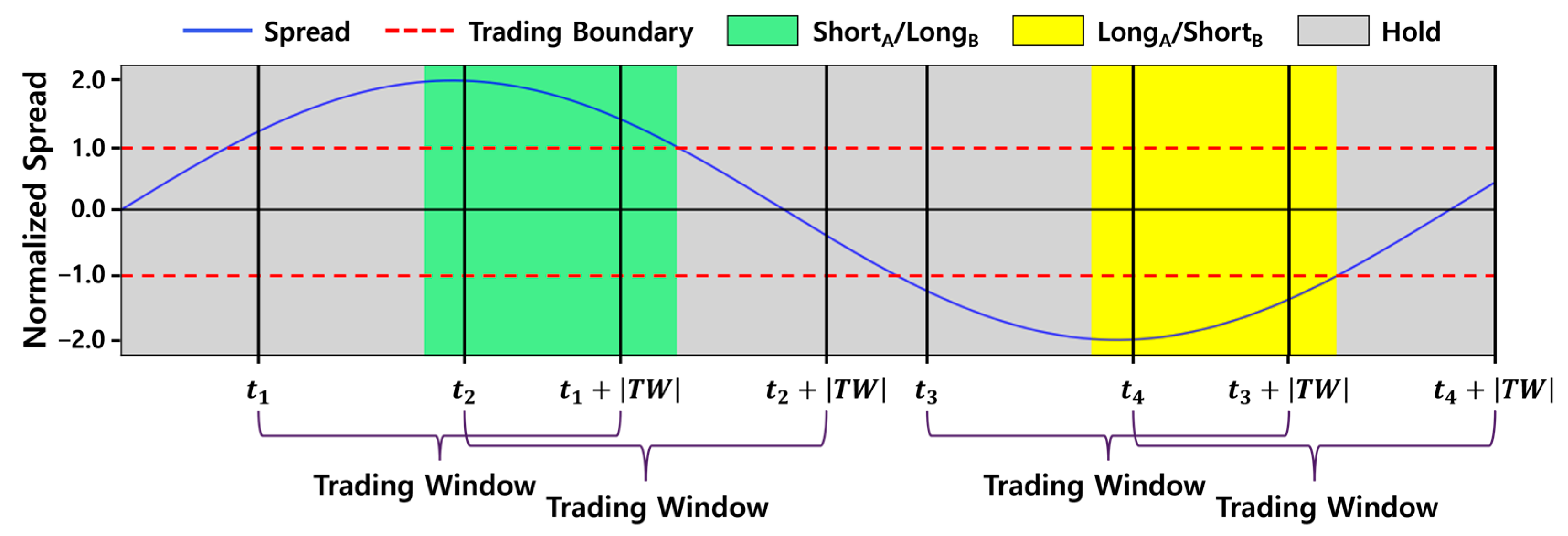
2.1. Pairs Trading
2.2. Reinforcement Learning
2.2.1. Deep Q-Network
2.2.2. Deep Deterministic Policy Gradient
2.2.3. Twin Delayed DDPG
3. Related Work
3.1. Algorithmic Trading
3.2. Pairs Trading
4. Hybrid Deep Reinforcement Learning for Pairs Trading
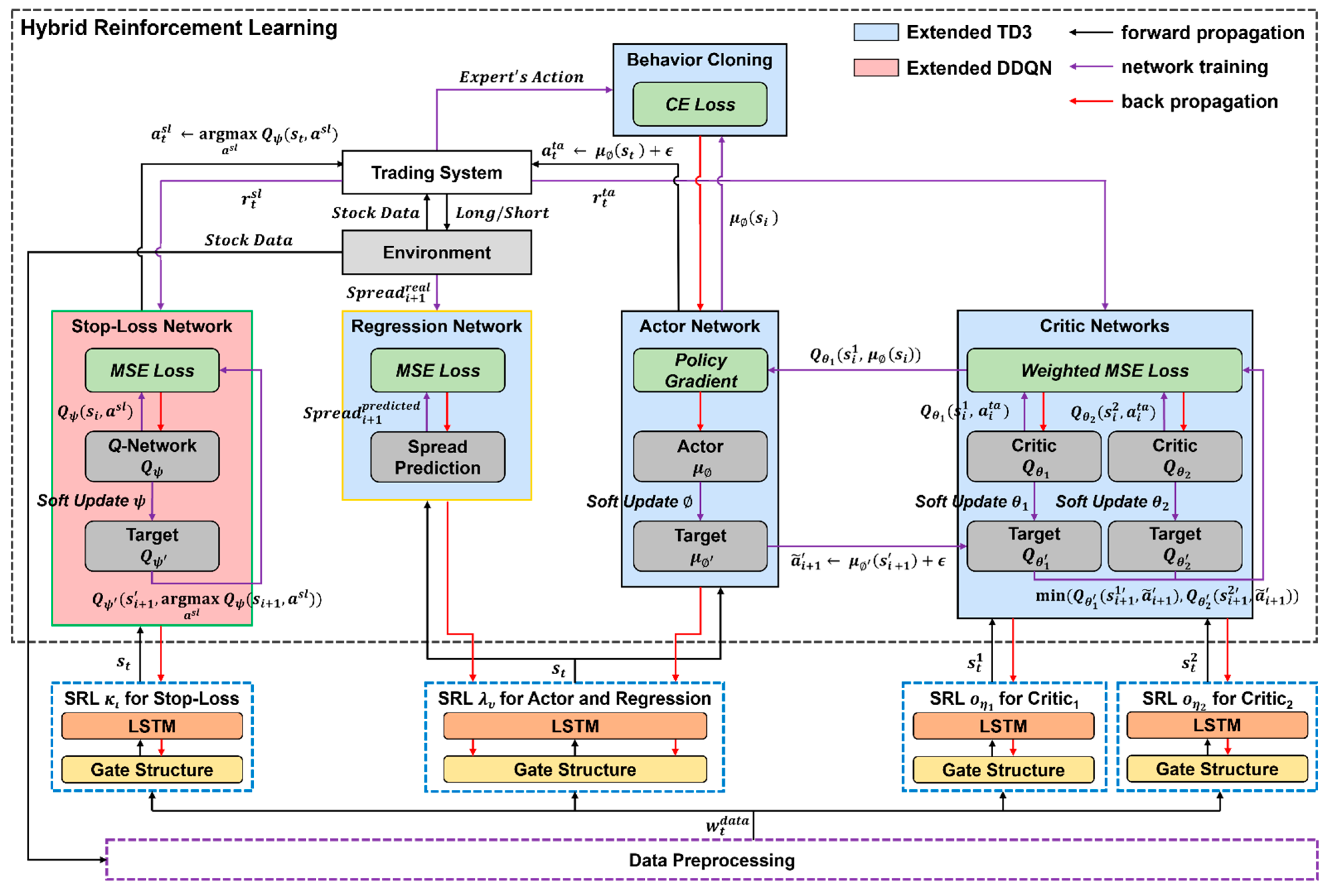
4.1. Architecture of HDRL-Trader
4.2. Data Preprocessing
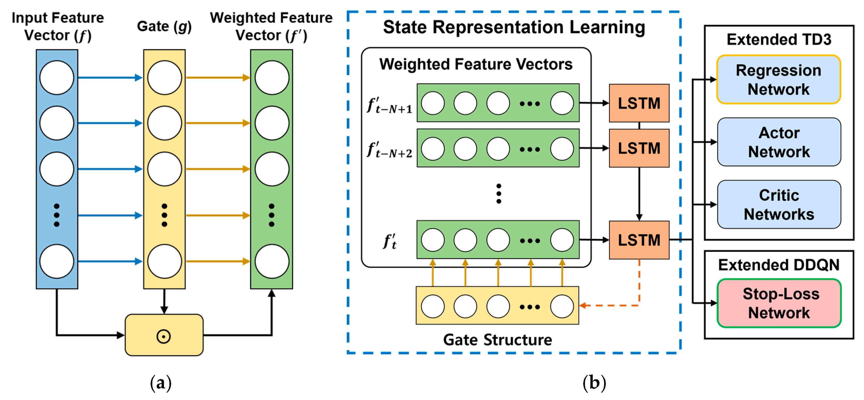
4.3. State Representation Learning
4.4. Hybrid Reinforcement Learning
4.4.1. Action Spaces for Pairs Trading
4.4.2. Reward Functions for Pairs Trading
4.4.3. Behavior Cloning
4.4.4. Hybrid Reinforcement Learning Algorithm
| Algorithm 1. The hybrid reinforcement learning algorithm of HDRL-Trader | |
| Input: Sliding-window data obtained from the data preprocessing | |
| Output: actor network , SRL network for , stop-loss network , SRL network | |
| 1. | Initialize an actor network , an SRL network for , and a regression network |
| 2. | Initialize critic networks , SRL networks for |
| 3. | Initialize a stop-loss network , an SRL network for |
| 4. | Initialize target networks: |
| 5. | Initialize a prioritized replay buffer |
| 6. | for |
| 7. | Compute the delay value for each epoch: |
| 8. | for t = 1 to T − 1 do |
| 9. | Select a trading action with exploration noise where |
| 10. | With probability , select a random stop-loss boundary |
| 11. | Otherwise, select where |
| 12. | Observe rewards and the next input |
| 13. | Store a transition where |
| 14. | Sample a minibatch of B transitions from with in Equation (8) |
| 15. | Smooth the target policy with where |
| 16. | where |
| 17. | Compute temporal difference errors: where |
| 18. | Update the critics by the MSE loss with the importance sampling weight in Equation (9) |
| 19. | Update the transition priority: |
| 20. | where |
| 21. | Update the stop-loss network by the MSE loss: where |
| 22. | if t mod d then |
| 23. | Update the actor by the deterministic policy gradient: |
| where | |
| 24. | Update the regression network by the MSE loss: |
| 25. | Update the actor by the CE loss for the behavior cloning: where |
| 26. | Soft-update the target networks: |
| 27. | end if |
| 28. | end for |
| 29. | end for |
4.5. Discussion
5. Experiments and Results
5.1. Experimental Setup
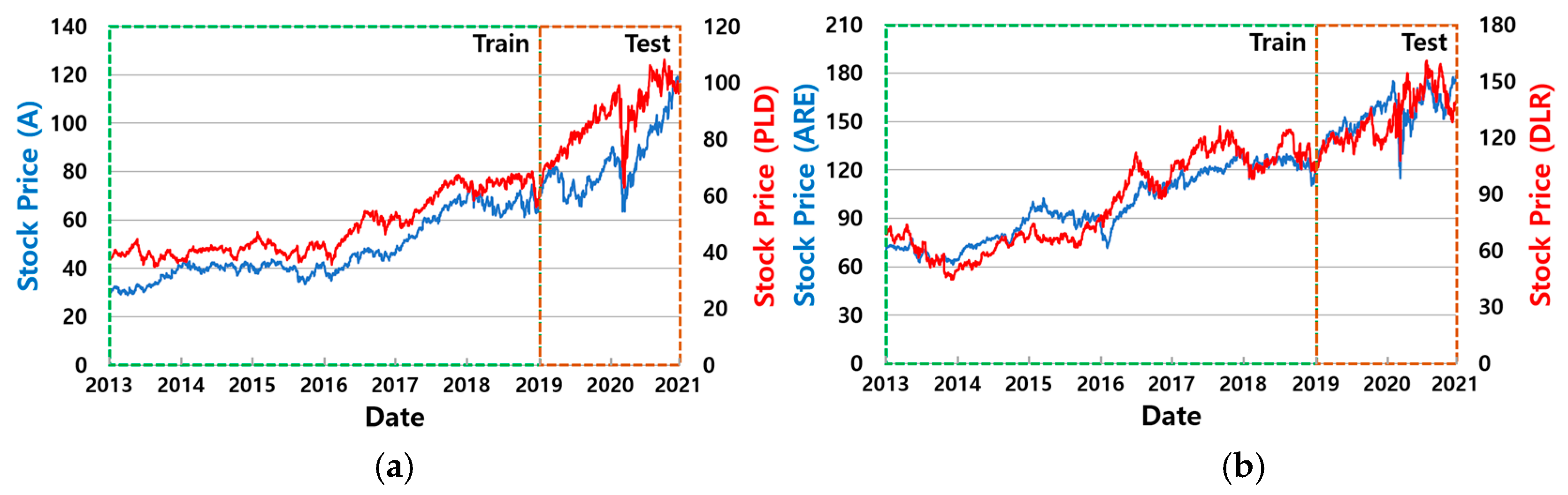
5.1.1. Datasets for Training and Testing
5.1.2. Evaluation Metrics
5.1.3. Baseline Methods
- Buy and Hold (B&H) buys two stocks in a pair on the first day of the test period, holds them, and then sells them on the last day of the test period.
- PTDQN [1] determines trading and stop-loss boundaries using a DQN. The Q-network comprises two ReLU dense layers with 15 units and a softmax output layer. We set the sliding window size to 30, mini-batch size to 32, learning rate to 0.001, and to 0.5 with a decay of 0.95.
- P-DDQN [3] determines trading actions using a DDQN with a negative reward multiplier. The Q-network comprises two ReLU dense layers with 50 units and a softmax output layer. We set the mini-batch size to 32, learning rate to 0.0001, and to 0.3.
- P-Trader [5] determines trading actions using a DDQN and employs techniques such as clustering, a gate structure, a temporal attention mechanism, and a regression network. The Q-network comprises two ReLU dense layers with 128 and 64 units and a softmax output layer. The regression network comprises a ReLU dense layer with 128 units and a linear output layer. We set the sliding window size to 15, mini-batch size to 32, learning rate to 0.0001, and to 0.5 with a decay of 0.95.
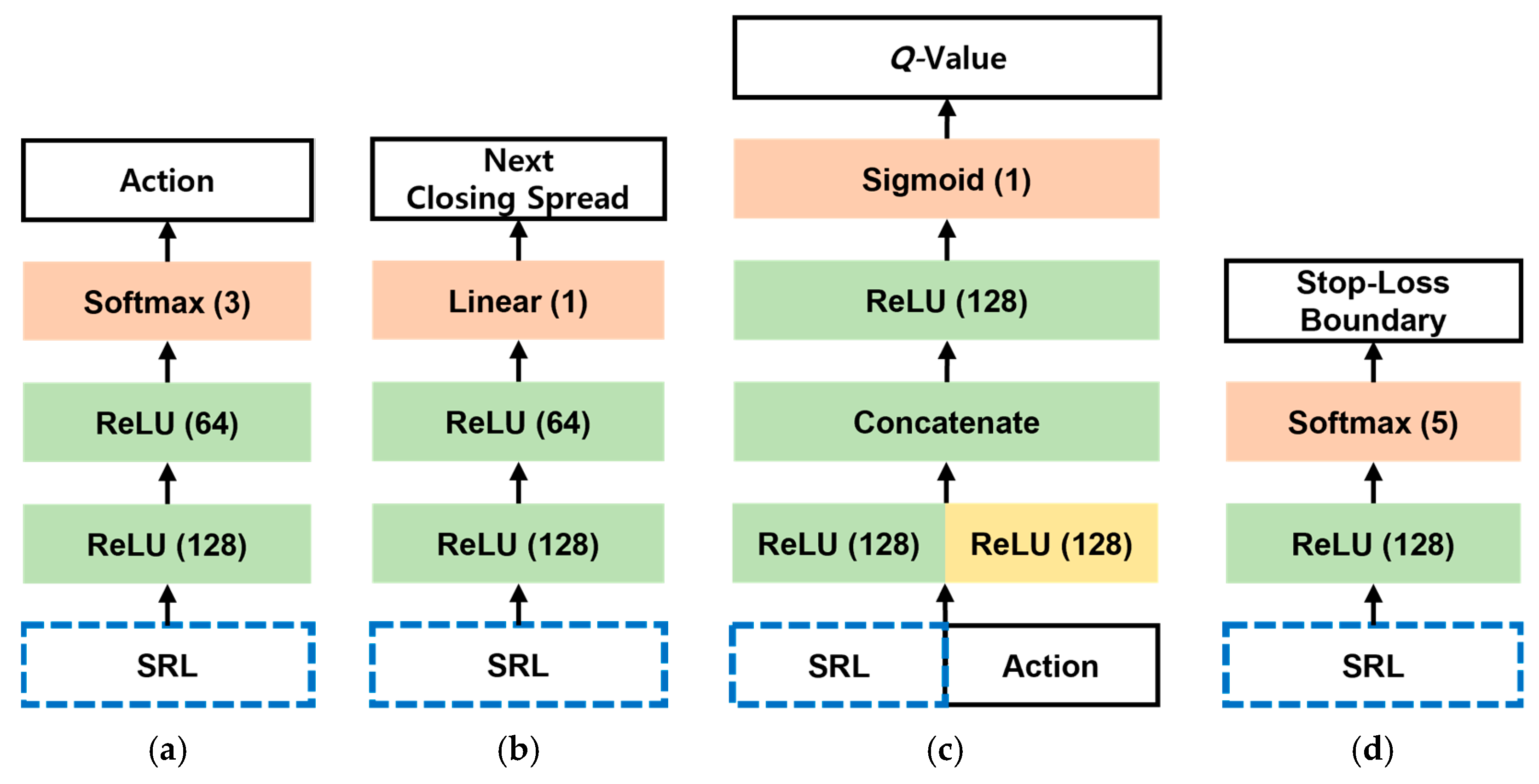
5.1.4. Implementation Details of HDRL-Trader
5.2. Experimental Results
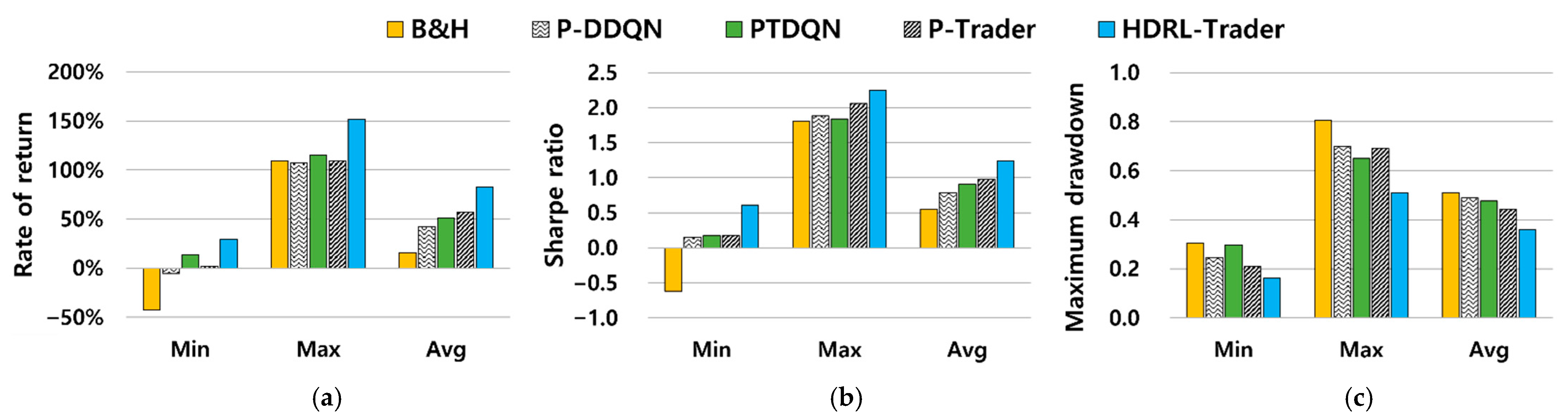
5.2.1. Comparison with Other Methods
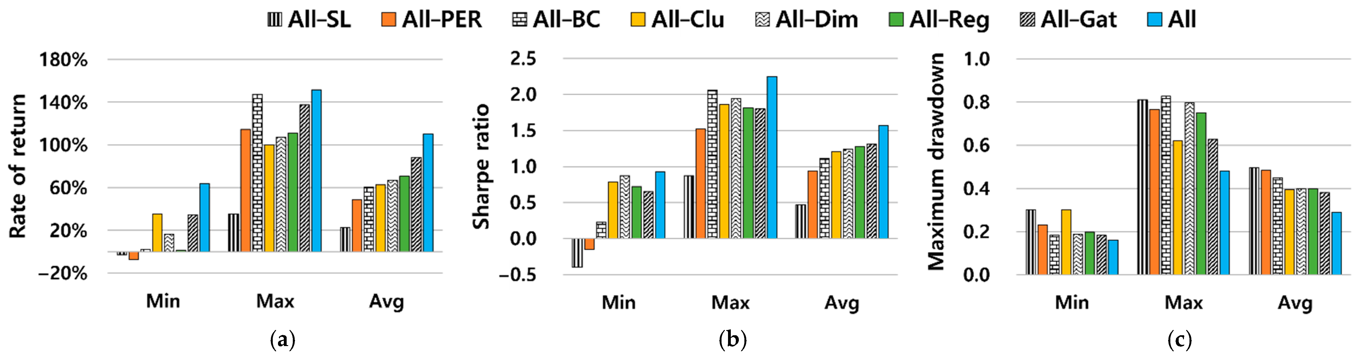
5.2.2. Ablation Studies
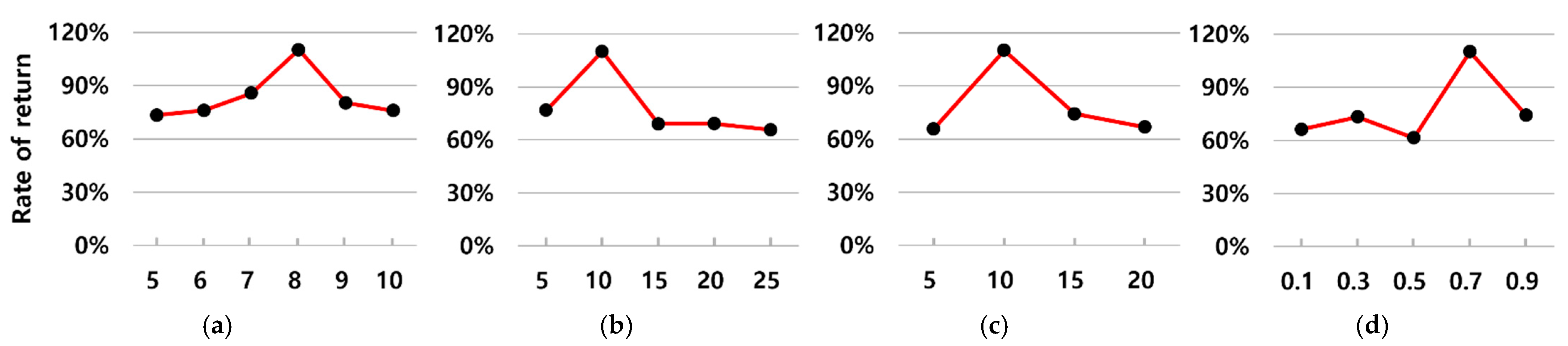
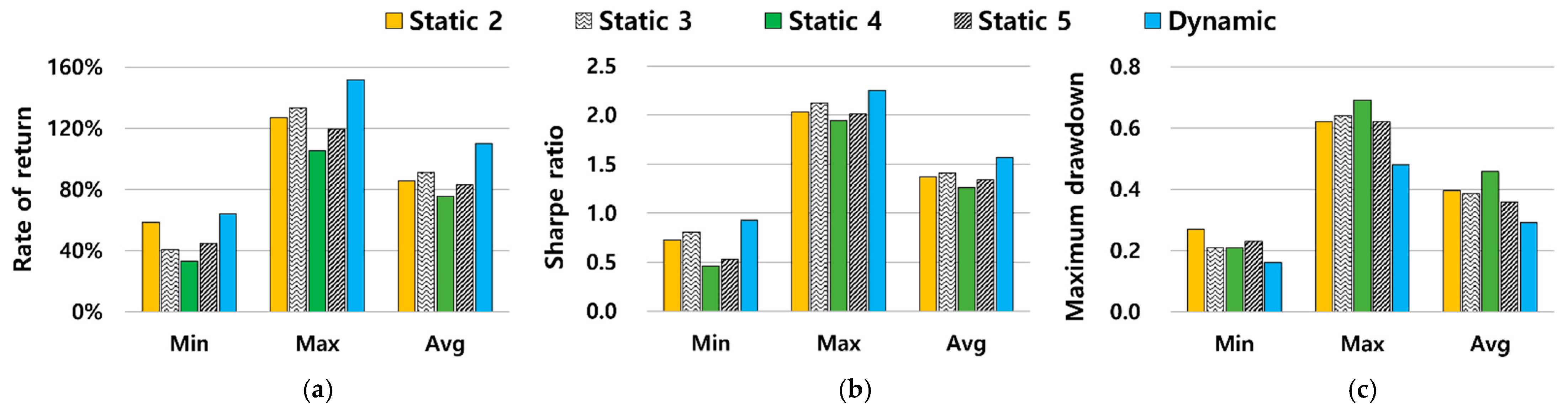
5.2.3. Comparison with Other Hyperparameter Values
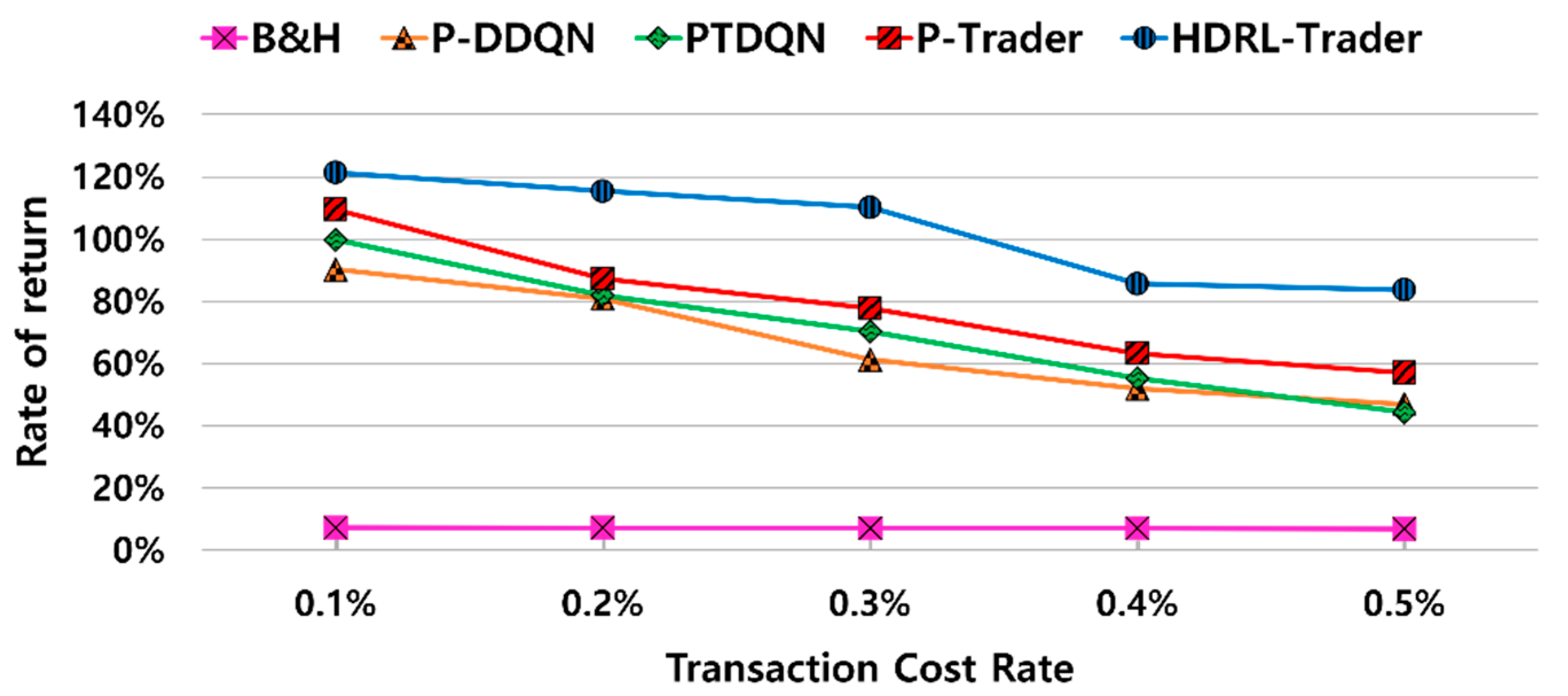
5.2.4. Robustness Study
6. Conclusions and Future Work
Author Contributions
Funding
Institutional Review Board Statement
Informed Consent Statement
Data Availability Statement
Conflicts of Interest
Appendix A

| Stock Pairs | Rate of Return | Sharpe Ratio | Maximum Drawdown | ||||||||||||
|---|---|---|---|---|---|---|---|---|---|---|---|---|---|---|---|
| B&H | P-DDQN | PT-DQN | P-Trader | HDRL-Trader | B&H | P-DDQN | PT-DQN | P-Trader | HDRL-Trader | B&H | P-DDQN | PT-DQN | P-Trader | HDRL-Trader | |
| AAPL, TXT | 109.3% | 88.8% | 109.6% | 99.8% | 125.2% | 1.81 | 1.51 | 1.74 | 1.72 | 2.12 | 0.58 | 0.63 | 0.57 | 0.54 | 0.47 |
| AOS, CCL | −15.4% | 51.6% | 13.4% | 50.0% | 68.4% | −0.04 | 0.37 | 0.17 | 0.54 | 0.86 | 0.59 | 0.49 | 0.64 | 0.69 | 0.51 |
| FE, RE | 53.8% | 20.7% | 43.3% | 57.9% | 65.3% | 1.20 | 0.55 | 1.07 | 0.98 | 1.05 | 0.41 | 0.42 | 0.36 | 0.39 | 0.27 |
| MMM, RE | 0.3% | 11.3% | 23.1% | 10.6% | 29.7% | 0.22 | 0.48 | 0.64 | 0.54 | 0.66 | 0.37 | 0.47 | 0.43 | 0.45 | 0.33 |
| NIKE, FTNT | 100.7% | 43.6% | 66.9% | 70.9% | 117.2% | 1.72 | 0.57 | 1.02 | 1.42 | 1.69 | 0.52 | 0.58 | 0.55 | 0.59 | 0.51 |
| SRE, MDT | 25.6% | 21.8% | 40.4% | 60.3% | 76.4% | 0.76 | 0.99 | 1.17 | 1.28 | 1.37 | 0.40 | 0.36 | 0.43 | 0.37 | 0.28 |
| APA, HES | −11.5% | 54.8% | 48.7% | 73.5% | 98.1% | 0.37 | 0.77 | 0.84 | 0.99 | 1.13 | 0.71 | 0.63 | 0.65 | 0.52 | 0.49 |
| OXY, HES | −23.5% | 57.3% | 29.3% | 44.3% | 60.1% | 0.16 | 0.95 | 0.65 | 0.81 | 1.06 | 0.68 | 0.51 | 0.47 | 0.55 | 0.46 |
| CMA, ADI | 25.7% | 11.1% | 16.8% | 23.3% | 51.4% | 0.69 | 0.55 | 0.56 | 0.64 | 0.94 | 0.46 | 0.61 | 0.56 | 0.45 | 0.34 |
| LHX, MTB | 14.4% | 33.1% | 21.0% | 40.0% | 53.2% | 0.53 | 0.63 | 0.54 | 0.65 | 0.84 | 0.40 | 0.33 | 0.30 | 0.32 | 0.21 |
| PEP, ATO | 20.3% | 1.1% | 15.4% | 37.4% | 51.8% | 0.68 | 0.32 | 0.43 | 0.75 | 0.86 | 0.30 | 0.40 | 0.48 | 0.36 | 0.30 |
| DXC, ALL | −9.1% | −5.5% | 28.3% | 2.0% | 29.0% | 0.09 | 0.15 | 0.49 | 0.17 | 0.61 | 0.54 | 0.60 | 0.53 | 0.52 | 0.47 |
| VLO, NTRS | −7.4% | 31.7% | 65.9% | 59.5% | 70.3% | 0.19 | 0.58 | 0.78 | 0.83 | 1.06 | 0.55 | 0.54 | 0.49 | 0.53 | 0.48 |
| MPC, CNC | −12.8% | 56.9% | 66.1% | 44.2% | 91.2% | 0.07 | 0.72 | 0.82 | 0.64 | 1.10 | 0.52 | 0.58 | 0.47 | 0.43 | 0.34 |
| A, PLD | 76.8% | 92.9% | 115.3% | 109.2% | 151.7% | 1.57 | 1.88 | 1.82 | 2.06 | 2.25 | 0.45 | 0.38 | 0.40 | 0.27 | 0.24 |
| ARE, DLR | 46.5% | 42.9% | 75.6% | 91.8% | 129.0% | 1.13 | 1.26 | 1.72 | 1.49 | 1.74 | 0.36 | 0.30 | 0.35 | 0.33 | 0.22 |
| O, EVRG | −0.4% | 27.8% | 51.8% | 49.6% | 79.8% | 0.25 | 0.82 | 0.98 | 0.86 | 1.25 | 0.43 | 0.25 | 0.39 | 0.21 | 0.16 |
| HIG, BK | 0.8% | 59.2% | 65.8% | 73.5% | 104.0% | 0.30 | 0.66 | 0.84 | 1.20 | 1.64 | 0.51 | 0.49 | 0.35 | 0.36 | 0.21 |
| COG, MRO | −42.8% | 107.0% | 104.5% | 99.1% | 132.3% | −0.62 | 1.49 | 1.16 | 1.33 | 1.61 | 0.65 | 0.70 | 0.59 | 0.46 | 0.43 |
| GPS, MRO | −38.2% | 37.8% | 13.7% | 37.5% | 64.0% | −0.12 | 0.54 | 0.48 | 0.63 | 0.93 | 0.81 | 0.51 | 0.53 | 0.52 | 0.48 |
| Minimum | −42.8% | −5.5% | 13.4% | 2.0% | 29.0% | −0.62 | 0.15 | 0.17 | 0.17 | 0.61 | 0.30 | 0.25 | 0.30 | 0.21 | 0.16 |
| Maximum | 109.3% | 107.0% | 115.3% | 109.2% | 151.7% | 1.81 | 1.88 | 1.82 | 2.06 | 2.25 | 0.81 | 0.70 | 0.65 | 0.69 | 0.51 |
| Average | 15.6% | 42.3% | 50.7% | 56.7% | 82.4% | 0.55 | 0.79 | 0.90 | 0.98 | 1.24 | 0.51 | 0.49 | 0.48 | 0.44 | 0.36 |
Appendix B
| Abbreviation | Description |
|---|---|
| B&H | Buy and Hold |
| CE | Cross Entropy |
| DPG | Deterministic Policy Gradient |
| DDPG | Deep Deterministic Policy Gradient |
| DQN | Deep Q-Network |
| DDQN | Double Deep Q-Network |
| GRU | Gated Recurrent Unit |
| LSTM | Long Short-Term Memory |
| MDP | Markov Decision Process |
| MSE | Mean Squared Error |
| SRL | State Representation Learning |
| HDRL | Hybrid Deep Reinforcement Learning |
| TD3 | Twin-Delayed Deep Deterministic policy gradient |
| TW | Trading Window |
References
- Kim, T.; Kim, H.Y. Optimizing the pairs-trading strategy using deep reinforcement learning with trading and stop-loss boundaries. Complexity 2019, 2019, 1–20. [Google Scholar] [CrossRef]
- Lu, J.Y.; Lai, H.C.; Shih, W.Y.; Chen, Y.F.; Huang, S.H.; Chang, H.H.; Wang, J.Z.; Huang, J.L.; Dai, T.S. Structural break-aware pairs trading strategy using deep reinforcement learning. J. Supercomput. 2021, 1–40. [Google Scholar] [CrossRef]
- Brim, A. Deep reinforcement learning pairs trading with a double deep Q-network. In Proceedings of the 2020 10th Annual Computing and Communication Workshop and Conference, CCWC, Las Vegas, NV, USA, 6–8 January 2020; pp. 222–227. [Google Scholar]
- Wang, C.; Sandås, P.; Beling, P. Improving pairs trading strategies via reinforcement learning. In Proceedings of the 2021 International Conference on Applied Artificial Intelligence, ICAPAI, Halden, Norway, 19–21 May 2021; pp. 1–7. [Google Scholar]
- Kim, S.H.; Park, D.Y.; Lee, K.H. A practical pairs-trading method using deep reinforcement learning. Database Res. 2021, 37, 65–80. [Google Scholar]
- Fujimoto, S.; Hoof, H.; Meger, D. Addressing function approximation error in actor-critic methods. In Proceedings of the 35th International Conference on Machine Learning, ICML, Stockholm, Sweden, 10–15 July 2018; Volume 80, pp. 1582–1591. [Google Scholar]
- Van Hasselt, H.; Guez, A.; Silver, D. Deep reinforcement learning with double Q-learning. In Proceedings of the 30th AAAI Conference on Artificial Intelligence, AAAI, Phoenix, AZ, USA, 12–17 February 2016; Volume 30, pp. 2094–2100. [Google Scholar]
- Dickey, D.A.; Fuller, W.A. Distribution of the estimators for autoregressive time series with a unit root. J. Am. Stat. Assoc. 1979, 74, 427–431. [Google Scholar]
- Sutton, R.S.; Barto, A.G. Reinforcement Learning: An Introduction; MIT Press: Cambridge, MA, USA, 2018. [Google Scholar]
- Kendall, E.A.; Malkoun, M.T.; Jiang, C.H. A methodology for developing agent based systems for enterprise integration. In Modelling and Methodologies for Enterprise Integration; Bernus, P., Nemes, L., Eds.; Springer: Boston, MA, USA, 1996; pp. 333–344. [Google Scholar]
- Slušný, S.; Neruda, R.; Vidnerová, P. Comparison of RBF network learning and reinforcement learning on the maze exploration problem. In Proceedings of the 18th International Conference on Artificial Neural Networks, ICANN, Prague, Czech Republic, 3–6 September 2008; pp. 720–729. [Google Scholar]
- Wang, B.N.; Gao, Y.; Chen, J.Y.; Chen, S.F. A two-layered multi-agent reinforcement learning model and algorithm. J. Netw. Comput. Appl. 2017, 30, 1366–1376. [Google Scholar] [CrossRef]
- Gershman, S.J.; Pesaran, B.; Daw, N.D. Human reinforcement learning subdivides structured action spaces by learning effector-specific values. J. Neurosci. 2009, 29, 13524–13531. [Google Scholar] [CrossRef] [PubMed] [Green Version]
- Kendall, E.A.; Malkoun, M.T.; Jiang, C.H. The application of object-oriented analysis to agent based systems. J. Occup. Organ. Psychol. 1997, 9, 56–62. [Google Scholar]
- Kaelbling, L.P.; Littman, M.L.; Cassandra, A.R. Planning and acting in partially observable stochastic domains. Artif. Intell. 1998, 101, 99–134. [Google Scholar] [CrossRef] [Green Version]
- Mnih, V.; Kavukcuoglu, K.; Silver, D.; Rusu, A.A.; Veness, J.; Bellemare, M.G.; Graves, A.; Riedmiller, M.A.; Fidjeland, A.K.; Ostrovski, G.; et al. Human-level control through deep reinforcement learning. Nature 2015, 518, 529–533. [Google Scholar] [CrossRef] [PubMed]
- Bellman, R. On the theory of dynamic programming. Proc. Natl. Acad. Sci. USA 1952, 38, 716–719. [Google Scholar] [CrossRef] [Green Version]
- Schaul, T.; Quan, J.; Antonoglou, I.; Silver, D. Prioritized experience replay. In Proceedings of the 4th International Conference on Learning Representations, ICLR, San Juan, Puerto Rico, 2–4 May 2016. [Google Scholar]
- Hessel, M.; Modayil, J.; Van Hasselt, H.; Schaul, T.; Ostrovski, G.; Dabney, W.; Horgan, D.; Piot, B.; Azar, M.; Silver, D. Rainbow: Combining improvements in deep reinforcement learning. In Proceedings of the 32nd AAAI Conference on Artificial Intelligence, (AAAI-18), New Orleans, LA, USA, 2–7 February 2018; pp. 3215–3222. [Google Scholar]
- Wang, Z.; Schaul, T.; Hessel, M.; Hasselt, H.; Lanctot, M.; Freitas, N. Dueling network architectures for deep reinforcement learning. In Proceedings of the 33rd International Conference on Machine Learning, ICML, New York, NY, USA, 19–24 June 2016; Volume 48, pp. 1995–2003. [Google Scholar]
- Sutton, R.S.; Barto, A.G. Introduction to Reinforcement Learning; MIT Press: Cambridge, MA, USA, 1998; Volume 135. [Google Scholar]
- Bellemare, M.G.; Dabney, W.; Munos, R. A distributional perspective on reinforcement learning. In Proceedings of the 34th International Conference on Machine Learning, ICML, Sydney, Australia, 6–11 August 2017; Volume 70, pp. 449–458. [Google Scholar]
- Fortunato, M.; Azar, M.G.; Piot, B.; Menick, J.; Hessel, M.; Osband, I.; Graves, A.; Mnih, V.; Munos, R.; Hassabis, D.; et al. Noisy networks for exploration. In Proceedings of the 6th International Conference on Learning Representations, ICLR, Vancouver, BC, Canada, 30 April–3 May 2018. [Google Scholar]
- Sutton, R.S.; McAllester, D.A.; Singh, S.P.; Mansour, Y. Policy gradient methods for reinforcement learning with function approximation. In Proceedings of the Advanced in Neural Information Processing Systems, NIPS, Denver, CO, USA, 29 November–4 December 1999; pp. 1057–1063. [Google Scholar]
- Silver, D.; Lever, G.; Heess, N.; Degris, T.; Wierstra, D.; Riedmiller, M. Deterministic policy gradient algorithms. In Proceedings of the 31st International Conference on Machine Learning, ICML, Beijing, China, 21–26 June 2014; Volume 32, pp. 387–395. [Google Scholar]
- Lillicrap, T.P.; Hunt, J.J.; Pritzel, A.; Heess, N.; Erez, T.; Tassa, Y.; Silver, D.; Wierstra, D. Continuous control with deep reinforcement learning. In Proceedings of the 4th International Conference on Learning Representations, ICLR, San Juan, Puerto Rico, 2–4 May 2016. [Google Scholar]
- Ding, X.; Zhang, Y.; Liu, T.; Duan, J. Deep learning for event-driven stock prediction. In Proceedings of the 24th International Joint Conference on Artificial Intelligence, IJCAI, Buenos Aires, Argentina, 25–31 July 2015; pp. 2327–2333. [Google Scholar]
- Tsantekidis, A.; Passalis, N.; Tefas, A.; Kanniainen, J.; Gabbouj, M.; Iosifidis, A. Forecasting stock prices from the limit order book using convolutional neural networks. In Proceedings of the 2017 IEEE 19th Conference on Business Informatics (CBI), Thessaloniki, Greece, 24–27 July 2017; Volume 1, pp. 7–12. [Google Scholar]
- Chong, E.; Han, C.; Park, F.C. Deep learning networks for stock market analysis and prediction: Methodology, data representations, and case studies. Expert Syst. Appl. 2017, 83, 187–205. [Google Scholar] [CrossRef] [Green Version]
- Zhang, L.; Aggarwal, C.; Qi, G.J. Stock price prediction via discovering multi-frequency trading patterns. In Proceedings of the 23rd ACM SIGKDD International Conference on Knowledge Discovery and Data Mining, KDD, New York, NY, USA, 13–17 August 2017; pp. 2141–2149. [Google Scholar]
- Tran, D.T.; Iosifidis, A.; Kanniainen, J.; Gabbouj, M. Temporal attention-augmented bilinear network for financial time-series data analysis. IEEE Trans. Neural Netw. Learn. Syst. 2018, 30, 1407–1418. [Google Scholar] [CrossRef] [PubMed] [Green Version]
- Feng, F.; He, X.; Wang, X.; Luo, C.; Liu, Y.; Chua, T.S. Temporal relational ranking for stock prediction. ACM Trans. Inf. Syst. 2019, 37, 1–30. [Google Scholar] [CrossRef] [Green Version]
- Fengqian, D.; Chao, L. An adaptive financial trading system using deep reinforcement learning with candlestick decomposing features. IEEE Access 2020, 8, 63666–63678. [Google Scholar] [CrossRef]
- Lei, K.; Zhang, B.; Li, Y.; Yang, M.; Shen, Y. Time-driven feature-aware jointly deep reinforcement learning for financial signal representation and algorithmic trading. Expert Syst. Appl. 2020, 140, 112872. [Google Scholar] [CrossRef]
- Liu, Y.; Liu, Q.; Zhao, H.; Pan, Z.; Liu, C. Adaptive quantitative trading: An imitative deep reinforcement learning approach. In Proceedings of the 34th AAAI Conference on Artificial Intelligence, AAAI, New York, NY, USA, 7–12 February 2020; Volume 34, pp. 2128–2135. [Google Scholar]
- Park, D.Y.; Lee, K.H. Practical algorithmic trading using state representation learning and imitative reinforcement learning. IEEE Access 2021, 9, 152310–152321. [Google Scholar] [CrossRef]
- Cho, K.; van Merrienboer, B.; Gülçehre, Ç.; Bahdanau, D.; Bougares, F.; Schwenk, H.; Bengio, Y. Learning phrase representations using RNN encoder-decoder for statistical machine translation. In Proceedings of the 2014 Conference on Empirical Methods in Natural Language Processing, EMNLP, Doha, Qatar, 25–29 October 2014; pp. 1724–1734. [Google Scholar]
- Li, T.; Zhao, Z.; Sun, C.; Cheng, L.; Chen, X.; Yan, R.; Gao, R.X. Waveletkernelnet: An interpretable deep neural network for industrial intelligent diagnosis. In IEEE Transactions on Systems, Man, and Cybernetics: Systems; IEEE: Piscataway, NJ, USA, 2021; pp. 1–11. [Google Scholar]
- Hochreiter, S.; Schmidhuber, J. Long short-term memory. Neural Comput. 1997, 9, 1735–1780. [Google Scholar] [CrossRef]
- Engle, R.F.; Granger, C.W.J. Co-integration and error correction: Representation, estimation, and testing. Econometrica 1987, 55, 251–276. [Google Scholar] [CrossRef]
- Liang, S.; Lu, S.; Lin, J.; Wang, Z. Low-latency hardware accelerator for improved Engle-Granger cointegration in pairs trading. IEEE Trans. Circuits Syst. I Regul. Pap. 2021, 68, 2911–2924. [Google Scholar] [CrossRef]
- Krauss, C. Statistical arbitrage pairs trading strategies: Review and outlook. J. Econ. Surv. 2016, 31, 513–545. [Google Scholar] [CrossRef]
- Brunetti, M.; Luca, R.D. Pre-Selection in Cointegration-Based Pairs Trading; Vergata Press: Italy, Rome, 2021. [Google Scholar]
- Miao, G.J. High frequency and dynamic pairs trading based on statistical arbitrage using a two-stage correlation and cointegration approach. Int. J. Econ. Financ. Issues 2014, 6, 96–110. [Google Scholar] [CrossRef] [Green Version]
- Chen, H.; Chen, S.; Chen, Z.; Li, F. Empirical investigation of an equity pairs trading strategy. Manag. Sci. 2017, 65, 370–389. [Google Scholar] [CrossRef] [Green Version]
- Erdem, O.; Ceyhan, E.; Varli, Y. A new correlation coefficient for bivariate time-series data. Phys. A Stat. Mech. Appl. 2014, 414, 274–284. [Google Scholar] [CrossRef]
- Bezdek, J.C.; Ehrlich, R.; Full, W. FCM: The fuzzy c-means clustering algorithm. Comput. Geosci. 1984, 10, 191–203. [Google Scholar] [CrossRef]
- TA-Lib: Technical Analysis Library. Available online: http://ta-lib.org/ (accessed on 22 November 2021).
- Li, W.; Liao, J. A comparative study on trend forecasting approach for stock price time series. In Proceedings of the 2017 11th IEEE International Conference on Anti-counterfeiting, Security, and Identification, ASID, Xiamen, China, 27–29 October 2017; pp. 74–78. [Google Scholar]
- Nabipour, M.; Nayyeri, P.; Jabani, H.; Mosavi, A.; Salwana, E.; Shahab, S. Deep learning for stock market prediction. Entropy 2020, 22, 840. [Google Scholar] [CrossRef] [PubMed]
- Banik, S.; Sharma, N.; Mangla, M.; Mohanty, S.N.; Shitharth, S. LSTM based decision support system for swing trading in stock market. Knowl.-Based Syst. 2021, 239, 107994. [Google Scholar] [CrossRef]
- Yahoo Finance. Available online: https://finance.yahoo.com/ (accessed on 22 November 2021).
- Sharpe, W.F. The Sharpe ratio. J. Portf. Manag. 1994, 21, 49–58. [Google Scholar] [CrossRef]
- Iantivics, L.B.; Iakovidis, D.K.; Nechita, E. II-Learn-A novel metric for measuring the intelligence increase and evolution of artificial learning systems. Int. J. Comput. Intell. Syst. 2019, 12, 1323–1338. [Google Scholar] [CrossRef] [Green Version]


| Feature Group | Features |
|---|---|
| Candlestick components [33] | Lengths of the upper shadow line, lower shadow line, and body; body color |
| Overlap studies [48] | BBANDS, DEMA, EMA, HT-TRENDLINE, KAMA, MA, MAMA, MIDPOINT, MIDPRICE, SAR, SAREXT, SMA, T3, TEMA, TRIMA, WMA |
| Momentum indicators [48] | ADX, ADXR, APO, AROON, AROONOSC, BOP, CCI, CMO, DX, MACD, MACDEXT, MACDFIX, MFI, MINUS_DI, MINUS_DM, MOM, PLUS_DI, PLUS_DM, PPO, ROC, ROCP, ROCR, RSI, STOCH, STOCHF, STOCHRSI, TRIX, ULTOSC, WILLR |
| Volume indicators [48] | AD, ADOSC, OBV |
| Volatility indicators [48] | ATR, NATR, TRANGE |
| Methods | Data Preprocessing | State Representation Learning | Reinforcement Learning | |||||
|---|---|---|---|---|---|---|---|---|
| Dim. Reduction | Clustering | Gating | Regression | Behavior Cloning | PER | Dynamic Delay | Hybrid | |
| HDRL-Trader | ○ | ○ | ○ | ○ | ○ | ○ | ○ | ○ |
| P-Trader [5] | × | ○ | ○ | ○ | × | × | × | × |
| PTDQN [1] | × | × | × | × | × | × | × | × |
| P-DDQN [3] | × | × | × | × | × | × | × | × |
| Rate of Return (the Higher the Better) | ||||||
|---|---|---|---|---|---|---|
| Stock Pairs | B&H | P-DDQN | PTDQN | P-Trader | HDRL-Trader | |
| Upward Trending | A, PLD | 76.8% | 92.9% | 115.3% | 109.2% | 151.7% |
| ARE, DRL | 46.5% | 42.9% | 75.6% | 91.8% | 129.0% | |
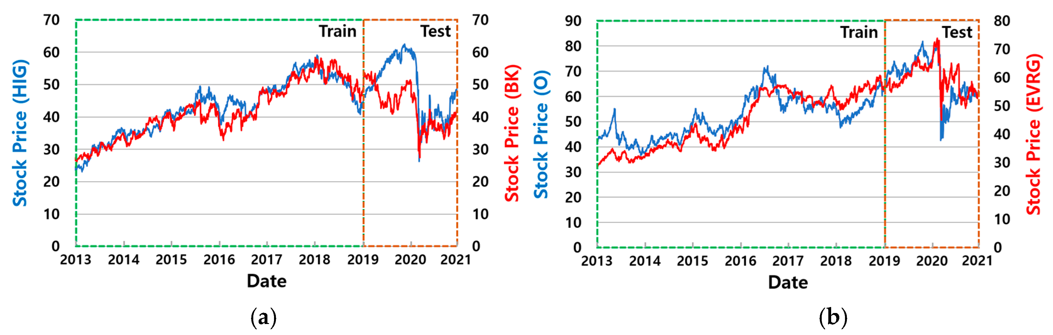
| Sideways Trending | HIG, BK | −0.4% | 27.8% | 51.8% | 49.6% | 79.8% |
| O, EVRG | 0.8% | 59.2% | 65.8% | 73.5% | 104.0% | |
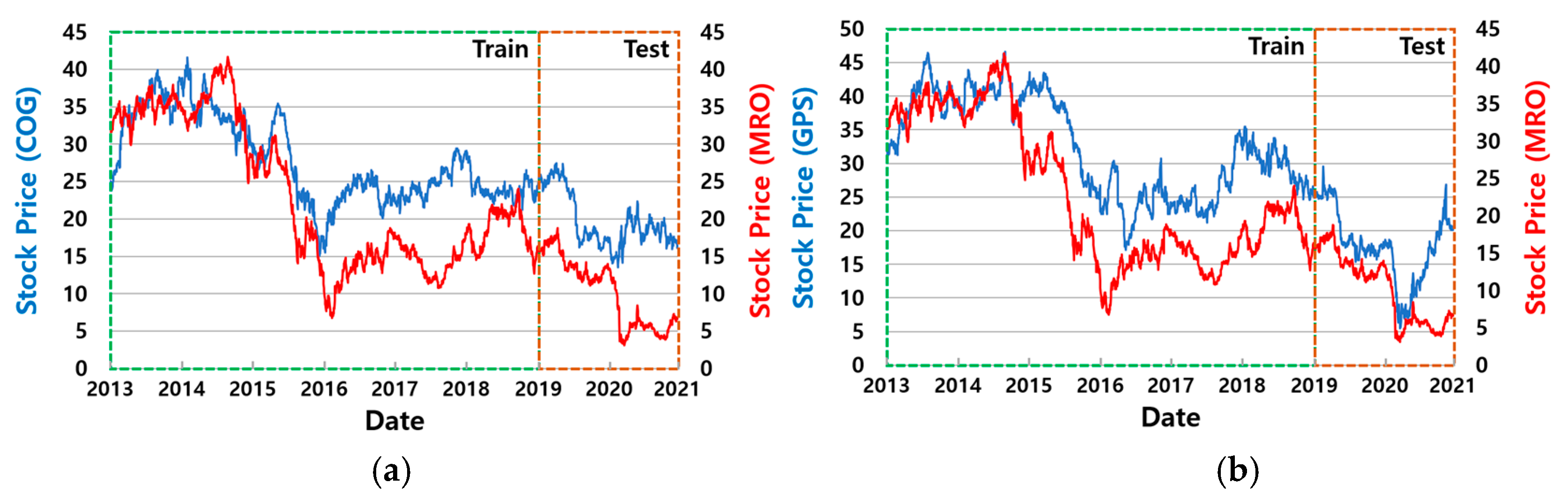
| Downward Trending | COG, MRO | −42.8% | 107.0% | 104.5% | 99.1% | 132.3% |
| GPS, MRO | −38.2% | 37.8% | 13.7% | 37.5% | 64.0% | |
| Minimum | −42.8% | 27.8% | 13.7% | 37.5% | 64.0% | |
| Maximum | 76.8% | 107.0% | 115.3% | 109.2% | 151.7% | |
| Average | 7.1% | 61.2% | 71.1% | 76.8% | 110.1% | |
| Sharpe Ratio (the Higher the Better) | ||||||
| Stock Pairs | B&H | P-DDQN | PTDQN | P-Trader | HDRL-Trader | |
| Upward Trending | A, PLD | 1.57 | 1.88 | 1.82 | 2.06 | 2.25 |
| ARE, DRL | 1.13 | 1.26 | 1.72 | 1.49 | 1.74 | |
| Sideways Trending | HIG, BK | 0.25 | 0.82 | 0.98 | 0.86 | 1.25 |
| O, EVRG | 0.30 | 0.66 | 0.84 | 1.20 | 1.64 | |
| Downward Trending | COG, MRO | −0.62 | 1.49 | 1.16 | 1.33 | 1.61 |
| GPS, MRO | −0.12 | 0.54 | 0.48 | 0.63 | 0.93 | |
| Minimum | −0.62 | 0.54 | 0.48 | 0.63 | 0.93 | |
| Maximum | 1.57 | 1.88 | 1.82 | 2.06 | 2.25 | |
| Average | 0.42 | 1.11 | 1.17 | 1.26 | 1.57 | |
| Maximum Drawdown (the Lower the Better) | ||||||
| Stock Pairs | B&H | P-DDQN | PTDQN | P-Trader | HDRL-Trader | |
| Upward Trending | A, PLD | 0.45 | 0.38 | 0.40 | 0.27 | 0.24 |
| ARE, DRL | 0.36 | 0.30 | 0.35 | 0.33 | 0.22 | |
| Sideways Trending | HIG, BK | 0.43 | 0.25 | 0.39 | 0.21 | 0.16 |
| O, EVRG | 0.51 | 0.49 | 0.35 | 0.36 | 0.21 | |
| Downward Trending | COG, MRO | 0.65 | 0.70 | 0.59 | 0.46 | 0.43 |
| GPS, MRO | 0.81 | 0.51 | 0.53 | 0.52 | 0.48 | |
| Minimum | 0.36 | 0.25 | 0.35 | 0.21 | 0.16 | |
| Maximum | 0.81 | 0.70 | 0.59 | 0.52 | 0.48 | |
| Average | 0.53 | 0.44 | 0.43 | 0.36 | 0.29 | |
Publisher’s Note: MDPI stays neutral with regard to jurisdictional claims in published maps and institutional affiliations. |
© 2022 by the authors. Licensee MDPI, Basel, Switzerland. This article is an open access article distributed under the terms and conditions of the Creative Commons Attribution (CC BY) license (https://creativecommons.org/licenses/by/4.0/).
Share and Cite
Kim, S.-H.; Park, D.-Y.; Lee, K.-H. Hybrid Deep Reinforcement Learning for Pairs Trading. Appl. Sci. 2022, 12, 944. https://doi.org/10.3390/app12030944
Kim S-H, Park D-Y, Lee K-H. Hybrid Deep Reinforcement Learning for Pairs Trading. Applied Sciences. 2022; 12(3):944. https://doi.org/10.3390/app12030944
Chicago/Turabian StyleKim, Sang-Ho, Deog-Yeong Park, and Ki-Hoon Lee. 2022. "Hybrid Deep Reinforcement Learning for Pairs Trading" Applied Sciences 12, no. 3: 944. https://doi.org/10.3390/app12030944
APA StyleKim, S.-H., Park, D.-Y., & Lee, K.-H. (2022). Hybrid Deep Reinforcement Learning for Pairs Trading. Applied Sciences, 12(3), 944. https://doi.org/10.3390/app12030944