Abstract
To fully consider the effect of elastic gasket (EG) on the segmental joint rotational behavior, an improved analytical approach is proposed to simulate the joint rotations and obtain the rotational stiffnesses. By comparing the analytical results with the experimental results and numerical results, the joint compression zone should be simulated by the concrete–EG–concrete (CGC) model instead of rigid–EG–rigid (RGR) model or concrete–concrete (CC) model. Since the analytical approach with the CGC model can simulate the combined work of EG and concrete well, it is a more effective approach to obtain the joint rotational stiffnesses. According to these analytical results, the EG has a great impact on softening the joint rotations, and this leads the rotational stiffnesses of the joint with EG to be evidently smaller than those of the joint without EG. In addition, with decreasing the axial force or increasing the EG thickness, this softening effect tends to be more obvious. Therefore, the EG is a significant factor which should be fully considered during the theoretical analysis for the joint rotation behavior, or it may lead to an unreliable design for the segmental lining.
1. Introduction
For the traffic, municipal, and water-conservancy projects extensively constructed throughout the world in recent decades, the shield method has been widely used in tunnel engineering. For the segmental lining, which is adapted for shield tunnels, the segmental joint is an important structure determining the bearing performance of the lining. As shown in Figure 1, the joint connects the adjacent segments with bolts, sealing gasket (SG), elastic gasket (EG), etc. Whether there is an EG is an important characteristic to distinguish the structure types of the segmental joints. For the segmental joint with EG, the EG packed in the joint can enhance the anti-seepage, alleviate the stress concentration, improve the flatness of the contact surface, etc. [1,2,3].
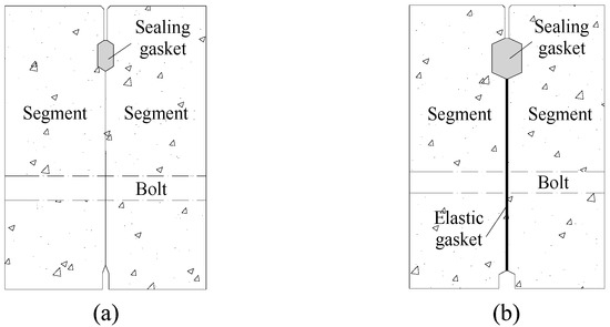
Figure 1.
Joint types: (a) joint without EG and (b) joint with EG.
The segmental joint is an important factor which can evidently affect the bearing performance of the whole lining. The mechanical mechanisms of the segmental joint are commonly described by three kinds of stiffnesses, which are rotational stiffness, axial stiffness, and shear stiffness in some analytical and numerical researches [4,5]. Since the axial stiffness and shear stiffness contribute little to the bearing performance of the segmental joint, they can be simplified or even ignored in structural analyses [6]. However, for the rotational stiffness, some numerical simulations [6] and experimental results [7] reveal that it can make a great contribution to the bearing performance of segmental joint; it is a key parameter to be considered in the structural design for the segmental lining [8]. Therefore, in recent years, an enormous amount of research effort goes into the joint rotations from the aspects of experimental test, numerical simulation, and theoretical analysis. These researches indicate that the joint rotations are very complex, and the joint rotational stiffnesses present obvious nonlinear characteristics with the influences of the complexity and diversity of segment joint types, structural dimensions, involved materials, and environmental conditions [9,10,11,12].
To calculate the joint rotation stiffness accurately, some analytical approaches are proposed for the segmental joints. As presented in Figure 2, in these approaches, the stresses of the bolt and SG are commonly assumed to be concentrated forces (Fb and Fs), and the stress distribution of the joint compression zone is assumed to be some simplified shapes to calculate the resultant force (Fc). Then, according to the equilibrium conditions of the joint axial force and bending moment, the joint rotational stiffnesses can be calculated. Obviously, an appropriate simplification of the stress distribution shape is the key to these approaches. For the joint without EG, as presented in Figure 2a, the concrete stress distribution can be assumed to be triangular, rectangular, trapezoidal, parabola, etc. [9,13,14,15,16,17,18]. The above approaches are also sometimes used for the joint with EG, while the influence of the EG is ignored in these cases. To take account of the EG, as presented in Figure 2b, the existing analytical approaches for the joint with EG are mainly based on the assumption that the concrete is much more rigid than EG, and the deformations of EG are much greater than those of the concrete. Therefore, only the compressive strains of EG are taken into consideration, while the compressive strains of the concrete attached to the EG are neglected [19,20,21,22,23,24]. In sum, this assumption only considers the stress generated by the compression of the EG instead of the concrete–EG–concrete composite structure. However, according to the constitutive model of EG, the rigidity of EG tends to be increased rapidly with increasing the compressive stress, and the EG can no longer be considered as a flexible material in this condition [16,25,26]. This leads to the result that, when the joints are subjected to large loads, the joint rotational stiffnesses calculated by the analytical approaches cannot coincide well with the numerical results [22,23,24]. Therefore, the deformations of the EG and the attached concrete should be both taken into consideration in the analytical approach to calculate the joint rotational stiffness.
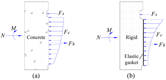
Figure 2.
Analytical approaches for the segmental joints: (a) joint without EG and (b) joint with EG.
This study aims to propose an improved analytical approach for the joint rotational behavior with fully consideration of the combined work of EG and concrete. To verify the proposed approach, the analytical results are compared with the experimental results and numerical results. Based on the analytical results, the bearing behavior of the segmental joint with EG is analyzed and compared with that of the segmental joint without EG, and the effect of EG on the joint bearing performance is clarified.
2. Analytical Approach for the Joint Rotational Behavior
2.1. Modeling Assumptions
Figure 3 presents the details of a typical segmental joint which is equipped with bolts, EG and SG. According to the condition of the stress transmission, the segmental joint can be classified as a few columnar functional zones. In most cases, the external or internal sides of joints can hardly be compressed in the vast majority of cases, unless the joint is subject to excessive loads [9,13,27]. Therefore, the functional zones at the external and internal edges can be assumed to be separate zones when the joint is subject to routine loads. In addition, since the SG stiffness is much smaller than that of the concrete and EG, the joint rotational stiffness is rarely influenced by the SG [9,25], and the SG transfer zone can be assumed to be merged into the separation zone. Therefore, the most significant bearing structures of the joint are the bolt and EG transfer zone. As shown in Figure 3b, the bolt is assumed to be a spring that can only be compressed, but not tensioned, and the EG transfer zone is assumed to be a concrete–EG–concrete composite columnar.
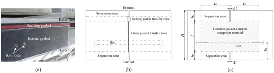
Figure 3.
Modeling assumptions: (a) segment, (b) joint details, and (c) assumptions.
2.2. Materials
2.2.1. Concrete
A multilinear isotropic hardening behavior is adopted for concrete. Its stress–strain relationship can be described as follows [28]:
where σc is the compressive stress in the concrete, ε0 is the strain at the compressive strength (fc) of the concrete, fcu,k denotes the characteristic value of the concrete compressive strength, and εcu indicates the maximum compressive strain of the concrete.
2.2.2. Bolt
The stress–strain behavior of the bolts is simplified to a bilinear kinematic hardening model with 1% strain hardening after yielding (), where and are the elastic modulus and plastic modulus, respectively. According to the following equations, the stress–strain relationship can be obtained.
where σb and fb are the stress and yield stress of the bolt, respectively.
2.2.3. Gasket
The constitutive model of the EG can be given by using the following equation [16,26], and the parameter in the equation can be calibrated by the compressive test of the EG.
where σe is the EG compressive stress, εe is the EG strain, Ee is the similar elastic module, and β is a nonlinear index number.
2.2.4. Composite
- Concrete–EG–concrete (CGC) model
According to the material models of concrete and EG, the stress–strain relationship of the concrete–EG–concrete composite material can be obtained by using the following equations:
where σ(ε) is the composite stress; ε is the composite strain; as presented in Figure 3c, lc is the depth of the composite compression zone and roughly equal to the height of the compression zone (l) [9,13,27]; and t is the EG thickness.
The maximum compressive strain (εu) of the composite can be calculated as follows:
- Rigid–EG–rigid (RGR) model
Some existing analytical approaches for the segmental joint with EG are mainly proposed based on the assumption that the concrete is much more rigid than the EG. For this assumption, only the compressive strains of the EG are taken into concertation, and the compressive strains of concrete attached to the EG are neglected. Therefore, the composite in Figure 3c can be considered as a rigid–EG–rigid (RGR) model, for which the concrete strain is approximately equal to zero. According to Equation (8), the strain of the composite can be presented as follows:
- Concrete–concrete (CC) model
For the segmental joint with EG, if the influence of the EG is neglected, it is regarded as the same as the joint without EG. Therefore, the composite in Figure 3c can be considered as a concrete–concrete (CC) model. In fact, this model is just a special case of the CGC model, and the thickness of the EG (t) in Equation (8) is equal to zero.
2.3. Equilibrium Equations
As shown in Figure 4, the height of the composite compression zone (l) is evenly divided into n sections, and the strains at the two edges are expressed as εe1 and εe2. Since the composite strain distribution presents linear characteristics, the strain in the center of each section i can be obtained as follows:
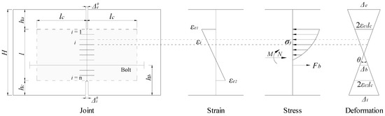
Figure 4.
Modeling approach.
The stress of each section i (σi) can be given by the stress–strain relationship of the composite material.
According to the equilibrium condition of the joint axial force and bending moment, we obtain the following:
From the joint deformation distribution presented in Figure 4, the following equation is obtained:
where Δb is the joint deformation at the bolt position. As shown in Equation (5), the bolt force (Fb) can be calculated by using the following:
where Lb is the effective length of the bolt, and Ab is the cross-sectional area of each bolt.
Based on the above equations, εe1 and εe2 can be calculated. Then the joint rotation angle can be presented as the following equation:
Since the concrete contact force at the joint edge was not considered in this study, the joint deformation at the compression edge should meet the following conditions:
where is the joint deformation at the compression side for the sagging moment scenario, is the initial gap between the two concrete segments at outside edges, is the joint deformation at the compression edge for the hogging moment scenario, and is the initial gap between the two concrete segments at the inside edges.
3. Validations of the Analytical Approach
3.1. Experimental Bending Tests
As presented in Figure 5, experimental bending tests of segmented joints were carried out by using two connected curved segments [29]. The horizontal loads (N) were applied by the MTS actuator, and vertical loads (P) were applied by the hydraulic jack. A roller support was positioned on the left end of the experimental structure, and a fixed support was positioned on the right. During the loading process, the eccentricity (e) was fixed to 150 mm, N increased gradually, and the corresponding P was calculated by the moment equilibrium of the joint.
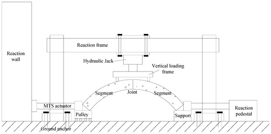
Figure 5.
Sketch view of the test setup [29].
The joint deformations are observed. The joint rotation angle (θ) is illustrated in Figure 6, and it can be calculated by using Equation (21). According to Equation (23), the rotational stiffness (Kθ) of the joint can be obtained by using the curve of the slope of the joint rotation angle (θ) versus the bending moment (M).
where δ1 is the averaged deformation at the opening edge, δ2 is the averaged deformation at the compression edges, and H is the segment thickness.
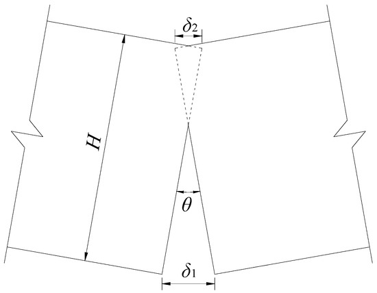
Figure 6.
Sketch view of the joint rotation angle.
For the segmental joint of the experimental structure, the related dimensions and materials are listed as the following.
Segment and joint: B = 1200 mm, H = 300 mm, ha = 80 mm, hb = 120 mm, hc = 40 mm, l = 180 mm, = 4 mm, and = 10 mm.
- Concrete: Type C50, and fc = 32.4 MPa.
- Bolt: n = 2, Eb = 210 GPa, Lb = 431 mm, Ab = 452.2 mm2, F0 = 20 kN, and fb = 640 MPa.
- EG: Ee = 2480 MPa, β = 1.67, t = 4 mm in the sagging-moment scenario, and t = 6 mm in the hogging-moment scenario.
3.2. Numerical Bending Tests
A three-dimensional (3D) numerical model was established for the experimental structure to reproduce the experimental bending tests. As presented in Figure 7, the numerical model of the joint with EG was established by using the software ANSYS. The concrete was simulated by using SOLID 65 elements. The bolt and SG were simulated by using SOLID 45 elements. The EG was simulated by using 3D interface elements (INTER 195), which can only be compressed in the normal direction. The contact interactions, including the interaction between the concrete and bolt, the interaction between the concrete and SG, and the interaction between the segment edges, were simulated by using “face-to-face” contacts. In most cases, the concrete friction coefficients ranged from 0.2 to 0.5 [30,31], and an average value of 0.35 was adopted in the simulation. As shown in Figure 7, to optimize the number of elements, only the elements near the joint were refined. The whole numerical model contains 203,912 elements and 43,148 nodes. To improve the convergence capability, the sparse direct solver was used for these nonlinear problems, and the maximum number of equilibrium iterations of each sub-step was increased to some extent.
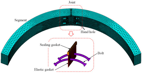
Figure 7.
Numerical model of the segmental joint with EG.
Furthermore, a 3D numerical model for the segmental joint without EG was established for supplementary bending tests. The numerical model of the concrete, bolts, and SG is exactly the same as the model of the segmental joint with EG. The only differences are that it does not contain EG, and the corresponding concrete is compressed by contacts during the loading process.
3.3. Comparison and Validation
3.3.1. Joint with Elastic Gasket
For the joint with EG, the stress–strain relationship of the CGC composite material in the analytical approach can be calculated by using Equations (7) and (8), and the stress–strain relationship of the RGR composite material can be calculated by using Equations (7), (8) and (10). If the influence of the EG is ignored, the stress–strain relationship of the composite material can be simplified as the CC model, which can be calculated directly by Equation (1). As presented in Figure 8, it is obvious that the CGC composite material is much softer than the CC material. That means the EG can have an effect on softening the joint, and by increasing the EG thickness, this effect tends to be more obvious. However, if the composite is simulated by the RGR model, the equivalent compression stiffness of the composite increases rapidly by increasing the compressive stress, and this is obviously inconsistent with the actual situation. Therefore, the EG, which is an important part of the joint, should be properly reflected in the calculation of the joint rotational stiffness.
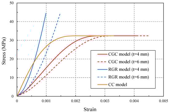
Figure 8.
Stress–strain relationship of the composite.
By applying an axial force to the joint, the rotation angle of the joint can be estimated by using the proposed analytical approach. According to the analytical results in Figure 9 and Figure 10, in the condition that the eccentricity (e) remains at 150 mm, with increasing the axial force constantly, the joint rotation angles tend to increase obviously in both the sagging-moment scenario and hogging-moment scenario. The experimental results and numerical results are also presented in Figure 9 and Figure 10. It can be seen that the differences between most of the numerical results and the corresponding experimental results are within 10%, which validates the reliability of the numerical simulations. According to the comparison, the curves from the analytical approach with the CGC model agree well with those from the experimental tests, for which the differences are within 13%. However, by increasing the axial force, the rotation angles calculated by the analytical approach with the RGR model tend to be much smaller than the experimental results; especially when the axial force increases to more than 500 kN, the maximum difference exceeds 20%. Therefore, the proposed analytical approach with the CGC model is more suitable than the RGR model for simulating the rotational behavior of the joint with EG.
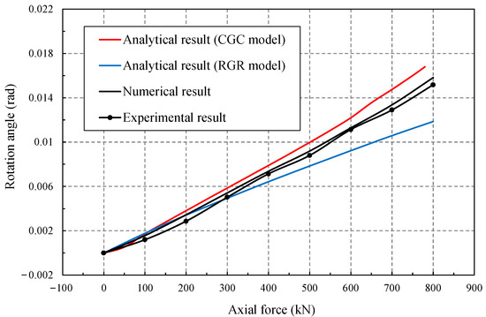
Figure 9.
Results for the joint with EG in sagging-moment scenario.
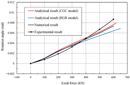
Figure 10.
Results for the joint with EG in hogging-moment scenario.
3.3.2. Joint without Elastic Gasket
For the joint without EG, the joint rotational behavior can be simulated by the proposed analytical approach with CC model. It can also be considered as a special case of the analytical approach with CGC model, for which the thickness of EG (t) is equal to zero. Using the analytical approach, the joint rotation angles are calculated when the joint is subject to different axial forces in the sagging-moment scenario and hogging-moment scenario. According to Figure 11 and Figure 12, when the axial forces are smaller than 500 kN, the curves from the analytical results with the CC model agree well with those from the numerical results, and the differences are within 10%. It is noteworthy that, with the increases of the axial forces, the differences between the analytical results and the numerical results tend to be increased, and this is also available to the results of the joint with EG (Figure 9 and Figure 10). Presumably it is because the plane–strain conditions are assumed for the proposed analytical approaches, leading to the avoidance of the three-dimensional effects. However, since the maximum difference does not exceed 14%, the proposed analytical approach can also be used to simulate the rotational behavior of the joint without EG.
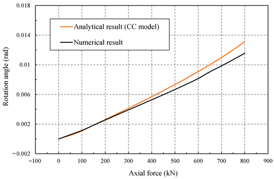
Figure 11.
Results for the joint without EG in sagging-moment scenario.
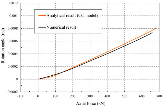
Figure 12.
Results for the joint without EG in hogging-moment scenario.
4. Parametric Study
When the segmental lining is in normal operation condition, the axial forces carried by the segmental joints are commonly stable. In this situation, according to Equation (23), the joint rotational stiffnesses can be obtained by the slopes of the joint-rotation-angle-versus-bending-moment curves when the joint is subject to a constant axial force. To compare the rotational behaviors of the joint with EG and the joint without EG, some parametric studies were performed by using the verified analytical approach, and the effect of the EG on the joint rotational stiffness was further investigated.
4.1. Effect of the Axial Force
The axial force (N) is always an important factor affecting the joint rotational behavior [6,9,32]. To investigate the effect of N on the rotational stiffnesses of the joint with EG and the joint without EG, the joint-rotation-angle-versus-bending-moment relationships with conditions that subject the joint to different axial forces are obtained. The joint-rotation-angle-versus-sagging-moment relationships with the axial forces of 500, 1000 and 1500 kN are presented in Figure 13. The joint-rotation-angle versus hogging-moment relationships with axial forces of 500, 1000 and 1500 kN are presented in Figure 14. According to the results in the two scenarios, by decreasing the axial force, the calculated rotation angles in the condition of the same bending moment are increased significantly. Therefore, according to Equation (23), the rotational stiffnesses of the two joints both tend to be significantly decreased. Moreover, with the condition of the same axial force, since the EG can have an effect on softening the joint rotational behavior, the average rotational stiffness of the joint with EG is smaller than that of the joint without EG. Moreover, with decreasing the axial force, the average distance between the rotation-angle-versus-bending-moment curves of the two joints subject to the same bending moment is increased gradually, thus indicating that the softening effect tends to be more significant.
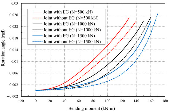
Figure 13.
Effect of N in sagging-moment scenario.
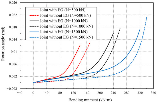
Figure 14.
Effect of N in hogging-moment scenario.
4.2. Effect of the EG Thickness
The effects of the EG thickness (t) on the joint rotational stiffnesses in the two scenarios were investigated for when the joint is subject to a constant axial force of 1000 kN. The joint-rotation-angle-versus-sagging-moment relationships with different thicknesses of 0 mm, 2 mm, 4 mm and 6 mm are presented in Figure 15. The joint-rotation-angle-versus-hogging-moment relationships with different thicknesses of 0 mm, 2 mm, 4 mm and 6 mm are presented in Figure 16. According to Figure 15 and Figure 16, in both the two scenarios, when the joint is subject to the same bending moment, the larger the EG thickness, the larger the joint rotation angle, and the smaller the rotational stiffness. Therefore, with increasing EG thickness, the effect of the EG on softening the joint rotational behavior tends to be more obvious in the two scenarios.
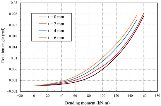
Figure 15.
Effect of t in sagging-moment scenario.
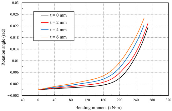
Figure 16.
Effect of t in hogging-moment scenario.
5. Conclusions
An improved analytical approach was proposed to simulate the segmental joint rotational behavior. The analytical results were compared with the experimental results and the numerical results. Using the analytical approach, the rotational stiffnesses of the joint with EG and the joint without EG were investigated, and the following conclusions were obtained.
(1) For the joint with EG, to fully consider the combined work of EG and concrete, the joint compression zone should be simulated by using the CGC model instead of the RGR model or CC model. Therefore, the proposed analytical approach with CGC model, which is verified by the experimental tests and numerical simulations, is a more effective approach to obtain the rotational stiffness of the joint with EG. Meanwhile, the proposed analytical approach with the CGC model can also be adapted to the joint without EG, since it can be assumed to be a special case that the thickness of EG is equal to zero.
(2) The EG has a significant effect on softening the joint rotational behavior, which can lead to the result that the average rotational stiffness of the joint with EG is evidently smaller than that of the joint without EG. Moreover, by decreasing the axial force or increasing the EG thickness, this softening effect tends to be more obvious. Therefore, there is a need to fully take into account the influence of EG on the joint rotational stiffness during the design of segment lining, or it will lead to larger designed joint rotational stiffness and potentially dangerous situations
Author Contributions
Conceptualization, F.Y.; methodology, F.Y.; software, F.Y.; validation, M.H. and F.Y.; formal analysis, M.H. and F.Y.; investigation, M.H. and F.Y.; resources, M.H.; data curation, M.H. and F.Y.; writing—original draft preparation, M.H. and F.Y.; writing—review and editing, M.H. and F.Y.; visualization, F.Y.; supervision, M.H.; project administration, M.H.; funding acquisition, F.Y. All authors have read and agreed to the published version of the manuscript.
Funding
This research was funded by the Fundamental Research Funds for the Central Universities, grant number JZ2020HGQA0141.
Data Availability Statement
Data will be made available by the corresponding author upon reason able request.
Conflicts of Interest
The authors declare no conflict of interest.
References
- Cho, S.H.; Kim, J.; Won, J.; Kim, M.K. Effects of Jack Force and Construction Steps on the Change of Lining Stresses in a TBM Tunnel. KSCE J. Civ. Eng. 2017, 21, 1135–1146. [Google Scholar] [CrossRef]
- Luciani, A.; Peila, D. Tunnel Waterproofing: Available Technologies and Evaluation Through Risk Analysis. Int. J. Civ. Eng. 2019, 17, 45–59. [Google Scholar] [CrossRef]
- Zhang, W.; Wang, B.; Zhang, G. The Influence of Dislocation on the Stress and Waterproof Performance of Shield Tunnel Joint. China Civ. Eng. J. 2020, 53, 63–68. [Google Scholar]
- Ding, W.Q.; Yue, Z.Q.; Tham, L.G.; Zhu, H.H.; Lee, C.F.; Hashimoto, T. Analysis of Shield Tunnel. Int. J. Numer. Anal. Met. 2004, 28, 57–91. [Google Scholar] [CrossRef]
- Lee, K.M.; Hou, X.Y.; Ge, X.W.; Tang, Y. An Analytical Solution for a Jointed Shield-driven Tunnel Lining. Int. J. Numer. Anal. Met. 2010, 25, 365–390. [Google Scholar] [CrossRef]
- Do, N.; Dias, D.; Oreste, P.; Djeran-Maigre, I. 2D Numerical Investigation of Segmental Tunnel Lining Behavior. Tunn. Undergr. Space Technol. 2013, 37, 115–127. [Google Scholar] [CrossRef]
- Arnau, O.; Molins, C. Experimental and Analytical Study of the Structural Response of Segmental Tunnel Linings Based on an in Situ Loading Test. Part 1: Test Configuration and Execution. Tunn. Undergr. Space Technol. 2011, 26, 764–777. [Google Scholar] [CrossRef] [Green Version]
- ITA. Guidelines for the Design of Shield Tunnel Lining. Tunn. Undergr. Space Technol. 2000, 15, 303–331. [Google Scholar] [CrossRef]
- Li, X.; Yan, Z.; Wang, Z.; Zhu, H. A Progressive Model to Simulate the Full Mechanical Behavior of Concrete Segmental Lining Longitudinal Joints. Eng. Struct. 2015, 93, 97–113. [Google Scholar] [CrossRef]
- Avanaki, M.J.; Hoseini, A.; Vahdani, S.; Fuente, A. Numerical-aided Design of Fiber Reinforced Concrete Tunnel Segment Joints Subjected to Seismic Loads. Constr. Build. Mater. 2018, 170, 40–54. [Google Scholar] [CrossRef]
- Wu, B.; Luo, Y.; Zang, J. Thermal Behavior of Tunnel Segment Joints Exposed to Fire and Strengthening of Fire-damaged Joints with Concrete-filled Steel Tubes. Appl. Sci. 2019, 9, 1781. [Google Scholar] [CrossRef] [Green Version]
- Lorenzo, S.G. The Role of Temporary Spear Bolts in Gasketed Longitudinal Joints of Concrete Segmental Linings. Tunn. Undergr. Space Technol. 2020, 105, 103576. [Google Scholar] [CrossRef]
- Janssen, P. Tragverhalten Von Tunnelausbauten Mit Gelenktübbings. Ph.D. Thesis, Technische Universität, Braunschweig, Germany, 1983. [Google Scholar]
- Koyama, Y. Study on the Improvement of Design Method of Segments for Shield-Driven Tunnels; RTRI Report: Special; RTRI: Tokyo, Japan, 2000; pp. 156–163. [Google Scholar]
- Blom, C. Design Philosophy of Concrete Linings for Tunnels in Soft Soils. Ph.D. Thesis, Technische Universiteit Delft, Delft, The Netherlands, 2002. [Google Scholar]
- Zhong, X.; Zhu, W.; Huang, Z.; Han, Y. Effect of Joint Structure on Joint Stiffness for Shield Tunnel Lining. Tunn. Undergr. Space Technol. 2006, 21, 406–407. [Google Scholar] [CrossRef]
- Shen, Y.; Yan, Z.; Zhu, H. An Analytical Mechanical Model for Tunnel Segmental Joints Subjected to Elevated Temperatures. In Proceedings of the International Symposium on Systematic Approaches to Environmental Sustainability in Transportation, Fairbanks, AK, USA, 2–5 August 2015; pp. 329–340. [Google Scholar] [CrossRef]
- Lei, M.; Lin, D.; Shi, C.; Ma, J.; Yang, W. A Structural Calculation Model of Shield Tunnel Segment: Heterogeneous Equivalent Beam Model. Adv. Civ. Eng. 2018, 2018, 9637838. [Google Scholar] [CrossRef] [Green Version]
- Zhang, H.; Guo, C.; Fu, D. A Study on the Stiffness Model of Circular Tunnel Prefabricated Lining. Chin. J. Geotech. Eng. 2000, 309–313. [Google Scholar] [CrossRef]
- Jiang, H.; Hou, X. Theoretical Study of Rotating Stiffness of Joint in Shield Tunnel Segments. Chin. J. Rock Mech. Eng. 2004, 23, 1574–1577. [Google Scholar] [CrossRef]
- Xia, C.; Zeng, G.; Bian, Y. Method for Determining Bending Stiffness of Shield Tunnel Segment Rings Longitudinal Joint Based on Fix-point Iteration. Chin. J. Rock Mech. Eng. 2014, 33, 901–912. [Google Scholar]
- Liu, T.J.; Huang, H.H.; Xu, R.; Tang, X.W.; Wang, S.Y. An Analytical Solution for the Failure Process of a Shield Tunnel Segmental Joint with a Load-transferring Gasket. In GSIC 2018: Proceedings of GeoShanghai 2018 International Conference: Tunnelling and Underground Construction; Zhang, D., Huang, X., Eds.; Springer: Singapore, 2018. [Google Scholar] [CrossRef]
- Yang, F.; Cao, S.; Li, Q. An Analytical Model for the Rotational Behavior of Concrete Segmental Lining Longitudinal Joints with Gaskets. Adv. Struct. Eng. 2019, 22, 2866–2881. [Google Scholar] [CrossRef]
- Yang, F.; Cao, S.; Qin, G. Simplified Spring Models for Concrete Segmental Lining Longitudinal Joints with Gaskets. Tunn. Undergr. Space Technol. 2020, 96, 103227. [Google Scholar] [CrossRef]
- Cavalaro, S.; Aguado, A. Packer Behavior under Simple and Coupled Stresses. Tunn. Undergr. Space Technol. 2012, 28, 159–173. [Google Scholar] [CrossRef]
- Zhang, J.; He, C. Analysis on Mechanical Properties of Segment Joints with Different Pressure Pads. J. China Rail. Soc. 2013, 35, 101–105. [Google Scholar] [CrossRef]
- Tvede-Jensen, B.; Faurschou, M.; Kasper, T. A Modelling Approach for Joint Rotations of Segmental Concrete Tunnel Linings. Tunn. Undergr. Space Technol. 2017, 67, 61–67. [Google Scholar] [CrossRef]
- GB 50010-2010(2015); Code for Design of Concrete Structures. China Architecture and Building Press: Beijing, China, 2010.
- Zhou, H.Y.; Chen, T.G.; Li, L.X. Study on Joint Bending Stiffness and Influencing Factors of Metro Shield Tunnelling Lining. Ind. Constr. 2010, 40, 59–61. [Google Scholar] [CrossRef]
- Arnau, O.; Molins, C. Three Dimensional Structural Response of Segmental Tunnel Linings. Eng. Struct. 2012, 44, 210–221. [Google Scholar] [CrossRef] [Green Version]
- Zhao, W.; Chen, W.; Yang, F. Study of the Interface Mechanical Properties of Concrete Segments in Shield Tunnels. Mod. Tunn. Technol. 2015, 52, 119–126. [Google Scholar] [CrossRef]
- Yuan, Q.; Liang, F.; Fang, Y. Numerical Simulation and Simplified Analytical Model for the Longitudinal Joint Bending Stiffness of a Tunnel Considering Axial Force. Struct. Concr. 2021, 22, 3368–3384. [Google Scholar] [CrossRef]
Publisher’s Note: MDPI stays neutral with regard to jurisdictional claims in published maps and institutional affiliations. |
© 2022 by the authors. Licensee MDPI, Basel, Switzerland. This article is an open access article distributed under the terms and conditions of the Creative Commons Attribution (CC BY) license (https://creativecommons.org/licenses/by/4.0/).