All You Need Is a Few Dots to Label CT Images for Organ Segmentation

Abstract

Image segmentation is used to analyze medical images quantitatively for diagnosis and treatment planning. Since manual segmentation requires considerable time and effort from experts, research to automatically perform segmentation is in progress. Recent studies using deep learning have improved performance but need many labeled data. Although there are public datasets for research, manual labeling is required in an area where labeling is not performed to train a model. We propose a deep-learning-based tool that can easily create training data to alleviate this inconvenience. The proposed tool receives a CT image and the pixels of organs the user wants to segment as inputs and extract the features of the CT image using a deep learning network. Then, pixels that have similar features are classified to the identical organ. The advantage of the proposed tool is that it can be trained with a small number of labeled data. After training with 25 labeled CT images, our tool shows competitive results when it is compared to the state-of-the-art segmentation algorithms, such as UNet and DeepNetV3.

1. Introduction

Image segmentation is used to analyze the medical image quantitatively for the quantification of tissue volume, diagnosis, treatment planning, and computer-integrated surgery [1]. However, it takes a lot of time and effort for a radiologist and doctor to conduct segmentation on CT images of each patient. Therefore, the necessity for technology that can accelerate segmentation on CT images has been highlighted consistently.

Over the past few decades, CNN-based deep learning techniques have made remarkable success in computer vision tasks, and there have been attempts to apply CNN-based methods in the field of medical image segmentation [2,3,4,5,6]. Afterward, UNet [7], which has the U-shaped encoder-decoder architecture with skip-connection, significantly improved the performance of the medical image segmentation task. Since the introduction of UNet, many variants using its architecture have been studied for segmentation tasks on organs and muscles of CT images in the medical field.

Although many deep learning models perform well enough to generate segmentation on CT images, it is not easy for medical institutions to train a network fit for their purpose. First, making public labeled data is difficult because the privacy of local data in medical institutions is essential. In addition, it cannot be guaranteed that the network trained by public data will conduct segmentation well on data owned by each institution since the distribution of pixels in the CT image differs depending on radiography equipment. Finally, the tedious work of labeling is needed whenever a segmentation task is conducted on an unlabeled organ in a public dataset.

In this research, we propose a deep-learning-based tool that can help with the labeling task, which is required to make the labeled data for a network performing segmentation and reduce the time and effort of experts. The network used for our tool can be trained with a small number of labeled data. After training, the tool shows the region of the organ when the user puts a dot on the target organ to be segmented. The user can conveniently adjust the threshold so that the labeling can be performed flexibly according to the data distribution. We expect that the labeled data for the medical image segmentation model would be easily made using our proposed labeling tool.

We compared our tool with two representative segmentation methods, UNet and DeepLabV3, for evaluation. Our technique is challenging to compare with the automated segmentation methods because a user has to annotate the pixels and set the threshold. Therefore, we proceed with two preceding experiments to determine the number of input anchors and the threshold for the experiment. For an efficient experiment, the anchors are extracted from the ground truth. Finally, Dice Score and Hausdorff Distance are used to measure the performance.

In this paper, our main contributions are as follows:

• We propose a novel labeling tool that can be trained with only a few labeled data by incorporating visual features and locality information extracted from Feature Encoder and Gaussian kernel.
• We utilize anchor pixels from user interactions for easily segmenting organs. The pixels can be selected anywhere on the target organs, with no additional constraints, such as annotating bounding-box, extreme points.
• Our tool provides an additional function to refine the segmentation result in detail by modifying the threshold value.

The following section discusses recent deep-learning-based segmentation models, interactive medical image segmentation models, and differences between the proposed method and existing interactive segmentation models. Section 3 introduces the proposed method, the dataset used for training, the metric for performance evaluation, and the application that can conveniently perform segmentation using our model. The results of measuring the performance of our method are presented in Section 4. Finally, Section 5 summarizes the proposed method and discusses future research directions.

2. Related Work

In this section, we study the recent work for image segmentation, which is categorized into UNet, Transformer-based models, and interactive segmentation methods. While many recent segmentation algorithms have adopted UNet and Transformer, they require a large set of fully labeled segmentation images. In this work, we exploit both UNet-based model architecture and an interactive segmentation strategy to generate a segmentation-labeled image with little effort.

2.1. Deep-Learning-Based Medical Image Segmentation

After the success of UNet on medical image segmentation tasks, there have been many studies trying to utilize its architecture or applying additional techniques to improve the performance [8,9,10,11]. For example, UNet combined with self-attention gates [8] on coarsely extracted feature maps from the encoding path is used for multi-organ segmentation. This gating method relieved the noisy response in skip-connection, capturing more precise textural and structural information on the input image patches. Bottleneck Feature supervised BS-UNet [9] connects its network with two UNets for liver and tumor segmentation. The first network is UNet with no skip-connection, which works as an auto-encoder learning the feature information from labeled data. The second network is the original UNet that performs the segmentation task. GIU-Net [12] utilize a graph-cut algorithm for multi-organ segmentation (skip-connection), which modified the structure of the skip-connection and used it to solve the task. Targeting organs-at-risk (OARs) is also crucial work in medical facilities. In [11], the convolution layers of UNet are replaced in the context aggregation block to learn from wide-range features to perform segmentation of OARs in cervical cancer.

Recently, research to improve medical image segmentation performance is still in progress. For instance, some studies adapt the UNet architecture as the backbone and exploit other deep learning techniques. UTNet [13] utilize a transformer encoder block and a decoder block as the last part of each convolution layer. Ref. [14] extracts fine-grained features by utilizing various sizes of the receptive field. It inserted a channel attention (CA) block into skip connection and applied a hybrid dilated attention convolutional (HDAC) layer to the last encoder output. X-Net [15] proposes an X-shaped network that can learn in parallel using two different branches: the CNN branch and transformer branch. As the Vision Transformer rises in various fields of the vision task, many studies utilizing vision transformers as the backbone have been conducted for medical image segmentation. In [16], a U-shaped network with a vision transformer base encoder for brain tumors and abdominal organ segmentation of 3D image patches is proposed, and a network consisting of pure transformers is introduced in [17]. The authors, inspired by Swin Transformer [18] and UNet, built an encoder-decoder architecture composed of only transformers using Swin Transformer blocks.

2.2. Interactive Medical Image Segmentation

Hence, interactive segmentation tools have been studied, which can assist in generating segmentation datasets on CT images with little effort. For instance, landmark points [19] or bounding boxes [20] could be guides for segmentation. Nevertheless, these studies still require many labeled data or careful guidance, which can make data collection expensive, especially in the medical field. Therefore, to solve such drawbacks, we propose an interactive labeling tool that can be helpful in the medical field, making it possible to gather data with ease and less time.

In addition, the performance of active contour models is also improved. Ref. [21] proposed an additive bias correction model to reduce the long execution time of the existing bias correction model. Since these active contour models must designate the region of interest (ROI) and detect the object’s boundary, the segmentation result can significantly differ depending on the given ROI. Our study focused on users conveniently performing segmentation on abdominal CT images.

3. Materials and Methods

We now define the dataset and propose our segmentation tool based on a deep neural network. Initially, we explain the CT image dataset used in this paper. Next, we introduce our model architecture consisting of a feature encoder and two kernel modules, the used metrics, and the loss function. Finally, we show our application implemented with these materials.

3.1. Dataset

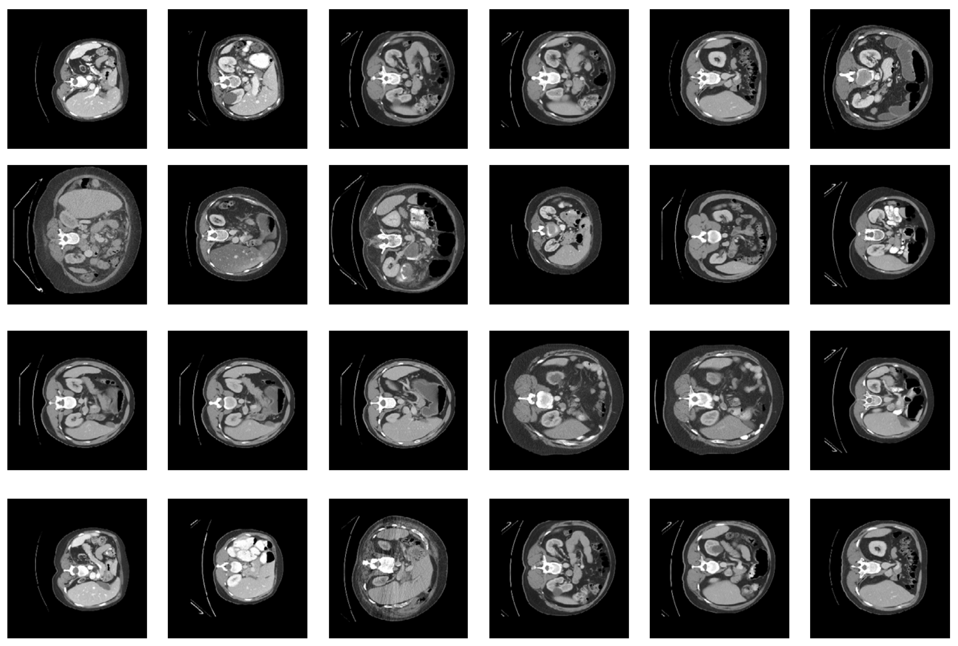
We utilize the BTCV [22] dataset (https://www.synapse.org/#!Synapse:syn3193805/files/, accessed on 1 September 2021). The dataset has 13 organs with segmentation performed by a trained person and reviewed by a radiologist. In this study, we measured the performance through four organs: liver, left kidney, right kidney, and spleen, located in the abdomen. In Figure 1, we provide abdominal CT images of four different people; each organ has its colors and textures, and the positions are relatively similar.

Figure 1. CT image examples that show different colors and textures for each organs.

To build our dataset, we sampled 202 CT images that have 4 organs: liver, spleen, left kidney, and right kidney. Among them, only 25 CT images were used for training and 177 CT images for testing. All CT images have segmentation labels. We exploited segmentation labels of the training set to randomly sample anchor pixels instead of manually picking them. For preprocessing, we arranged the range of CT image pixels to [−1, 1] and applied histogram equalization.

3.2. Proposed Method

We propose a semi-automated tool that generates organ segmentation. Given a CT image, the radiologists annotate a few pixels—an anchor to specify the target organ. The pixels near the anchor pixels, which have similar characteristics, are candidates of the target organ to be segmented. To capture the segmentation region of the target organs, we utilize two types of information: visual features and locality. 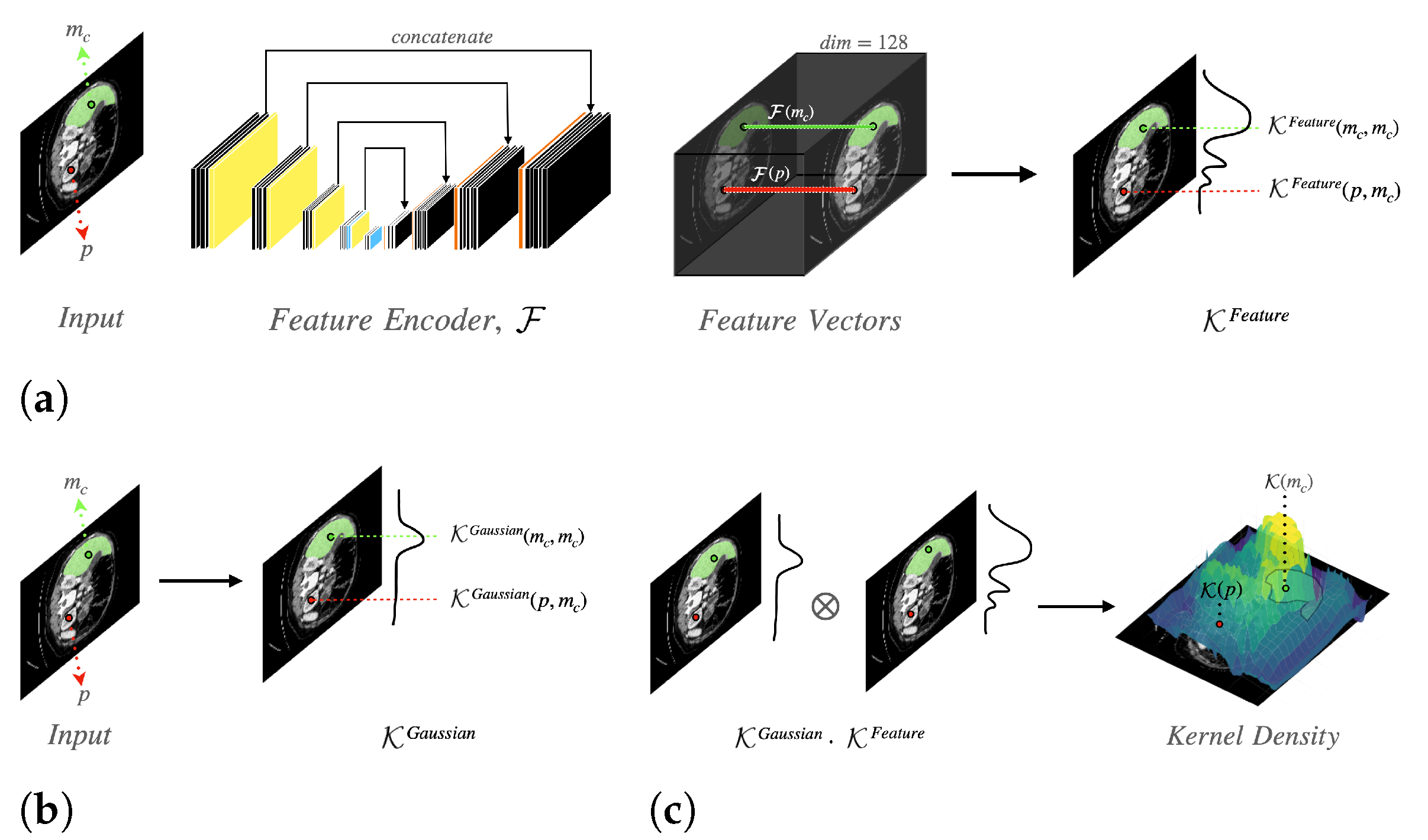In Figure 2, we provide a schematic representation of our network. Our proposed model consists of two sub-modules: Feature Encoder $\mathcal{F}$ and Kernel Function $\mathcal{K}$. The Feature Encoder $\mathcal{F}$ extracts the feature vector for each pixel, which is used to calculate the visual similarity between pixels. We exploit a modified U-Net architecture to implement the Feature Encoder $\mathcal{F}$.

Figure 2. Model architecture that consists of 2 kernels. These kernels are used to compute the kernel density, which has a high value in the region of the target organ: (a) Feature similarity kernel density; (b) Gaussian kernel density; (c) Kernel density.

The Kernel Function $\mathcal{K}$ is used to capture both visual features and locality information. In a CT image, let $M_c$ be a set of anchor pixels that a user picks on the c-th organ. The Kernel Function $\mathcal{K}$ computes the density for all pixels, which represents visual and positional similarity. As illustrated in Figure 2c, the kernel density is made of two types of densities: feature similarity kernel density ${\mathcal{K}}_c^{\mathrm{Feature}}$ (shown in Figure 2a) and Gaussian kernel density ${\mathcal{K}}_c^{\mathrm{Gaussian}}$ (shown in Figure 2b). The kernel density${\mathcal{K}}_c$ of a pixel p is computed as follows:

$$\begin{array}{c}\hfill {\mathcal{K}}_c\left(p\right)=\sum _{m_c\in {\mathbf{M}}_c}{\mathcal{K}}_c^{\mathrm{Feature}}(p,m_c){\mathcal{K}}_c^{\mathrm{Gaussian}}(p,m_c)\end{array}$$

(1)

where p is an arbitrary pixel, and $m_c$ is an anchor pixel of the c-th organ. ${\mathcal{K}}_c^{\mathrm{Feature}}$ means the feature similarity kernel density for the c-th organ. The feature similarity kernel density measures the feature similarity of two pixels. ${\mathcal{K}}_c^{\mathrm{Gaussian}}$ indicates the Gaussian kernel density for the c-th organ. The Gaussian kernel density calculates the positional similarity of two pixels.

The kernel density has a maximum value at each anchor pixel $m_c$. In the other case, the density value becomes high if a pixel p is closer to the anchor pixels ${\mathbf{M}}_c$ and has a similar texture or color too. Therefore, we can figure out the region of the c-th organ, filtering pixels with a high density.

If a pixel p has similar visual features to anchor pixels $M_c$, the pixel p is more likely to belong to the c-th organ than other pixels. Using feature vectors $\mathcal{F}\left(p\right)$ for the pixel p and $\mathcal{F}\left(m_c\right)$ for an anchor pixel $m_c$, we can calculate the feature similarity kernel density by using the dot product between $\mathcal{F}\left(p\right)$ and $\mathcal{F}\left(m_c\right)$ as follows:

$$\begin{array}{c}\hfill {\mathcal{K}}_c^{\mathrm{Feature}}(p,m_c)=\mathcal{F}{\left(p\right)}^T·\mathcal{F}\left(m_c\right)\end{array}$$

(2)

where p is an arbitrary pixel, and $m_c$ is an anchor pixel in the c-th organ. The operator · means dot product. If two pixels p and $m_c$ have similar features, the feature similarity kernel density has high value.

Gaussian kernel quantified how close the pixel is to anchor points, that is, a pixel closer to anchor pixels has a higher density value. This density is required not to capture regions that have similar texture but are far from anchor points (in another organ). A pixel p should be closer to anchor pixels for being classified as a target label. The Gaussian kernel density is calculated as follows:

$$\begin{array}{c}\hfill {\mathcal{K}}_c^{\mathrm{Gaussian}}(p,m_c)=exp(-{\gamma }_c\left|\right|p-m_c{\left|\right|}_2^2)\end{array}$$

(3)

where ${\gamma }_c$ is a trainable precision parameter used in Gaussian kernel for the c-th organ, and $\left|\right|·{\left|\right|}_2$ indicates $L_2$ norm.

In practice, we exploit a modified UNet architecture used as the Feature Encoder. We replace the convolution layers with the same padded convolution layers to fit the output resolution to the input resolution. We changed the output feature map channel to 128, which is the length of the feature vector of a pixel. Lastly, we utilize the Adam optimizer [23] to train our model.

3.3. Loss Function

We utilize Noise Contrastive Estimation (NCE) [24] loss to build the objective function. NCE loss uses negative sampling to optimize model parameters by forcing the density of the positive sample to be high and the density of the negative sample to be low. Let ${\mathbf{P}}_c^{pos}$ be a set of pixels in the c-th organ and ${\mathbf{P}}_c^{neg}$ be a set of pixels not in the c-th organ. We collected positive pixels $p_c^{pos}$ by randomly sampling from ${\mathbf{P}}_c^{pos}$ and collected negative pixels $p_c^{neg}$ in the same way from ${\mathbf{P}}_c^{neg}$. Using these pixels, we formulate the NCE loss, whose form is from InfoNCE loss [25], as follows:

$$\begin{array}{c}\hfill {\mathcal{L}}_{NCE}=\sum _c\mathcal{L}\left(c\right)\end{array}$$

(4)

$$\begin{array}{c}\hfill \mathrm{where}\mathcal{L}\left(c\right)={\mathbb{E}}_{p_c^{pos}\sim {\mathbf{P}}_c^{pos}}\left[-log\frac{exp\left({\mathcal{K}}_c\left(p_c^{pos}\right)\right)}{{\mathbb{E}}_{p_c^{neg}\sim {\mathbf{P}}_c^{neg}}\left[exp({\mathcal{K}}_c\left(p_c^{neg}\right)\right]}\right]\end{array}$$

(5)

where ${\mathcal{L}}_c$ is the NCE loss for the c-th organ, $p_c^{pos}$ is a pixel in the c-th organ, and $p_c^{neg}$ is a pixel not in the c-th organ. ${\mathcal{K}}_c(·)$ indicates the kernel density of a pixel, and $\mathbb{E}[·]$ means the expectation.

3.4. Evaluation Metrics

To evaluate the performance of our model, we compare it with two baseline models: UNet and DeepNet-V3. We benchmark the segmentation performance with two segmentation measures: dice score and Hausdorff distance. Given the predicted region P and ground truth region G, the dice score is computed as follows:

$$\begin{array}{c}\hfill DICE=\frac{2(P\cap G)}{\left|P\right|+\left|G\right|}\end{array}$$

(6)

where $\left|P\right|$ and $\left|G\right|$ mean the cardinality of P and G, respectively. The dice score indicates overlapped area between the segmentation prediction and ground truth, penalizing the missing prediction. In case the model prediction is more similar to ground truth in terms of segmentation size, the dice score is more highly evaluated. The Hausdorff distance is computed as follows:

$$\begin{array}{c}\hfill HD(P,G)=max(\underset{p\in P}{max}\underset{g\in G}{min}\Vert p-g\Vert ,\underset{g\in G}{max}\underset{p\in P}{min}\Vert g-p\Vert )\end{array}$$

(7)

In the inner terms, the first term calculates the maximum distance to the minimum distance from the predicted pixel to the ground truth pixel, and the second term calculates the distance. As a result, the Hausdorff distance represents the maximum distance between two pixels and that each pixel belongs to the exclusive region, respectively.

3.5. The Application Generating Label

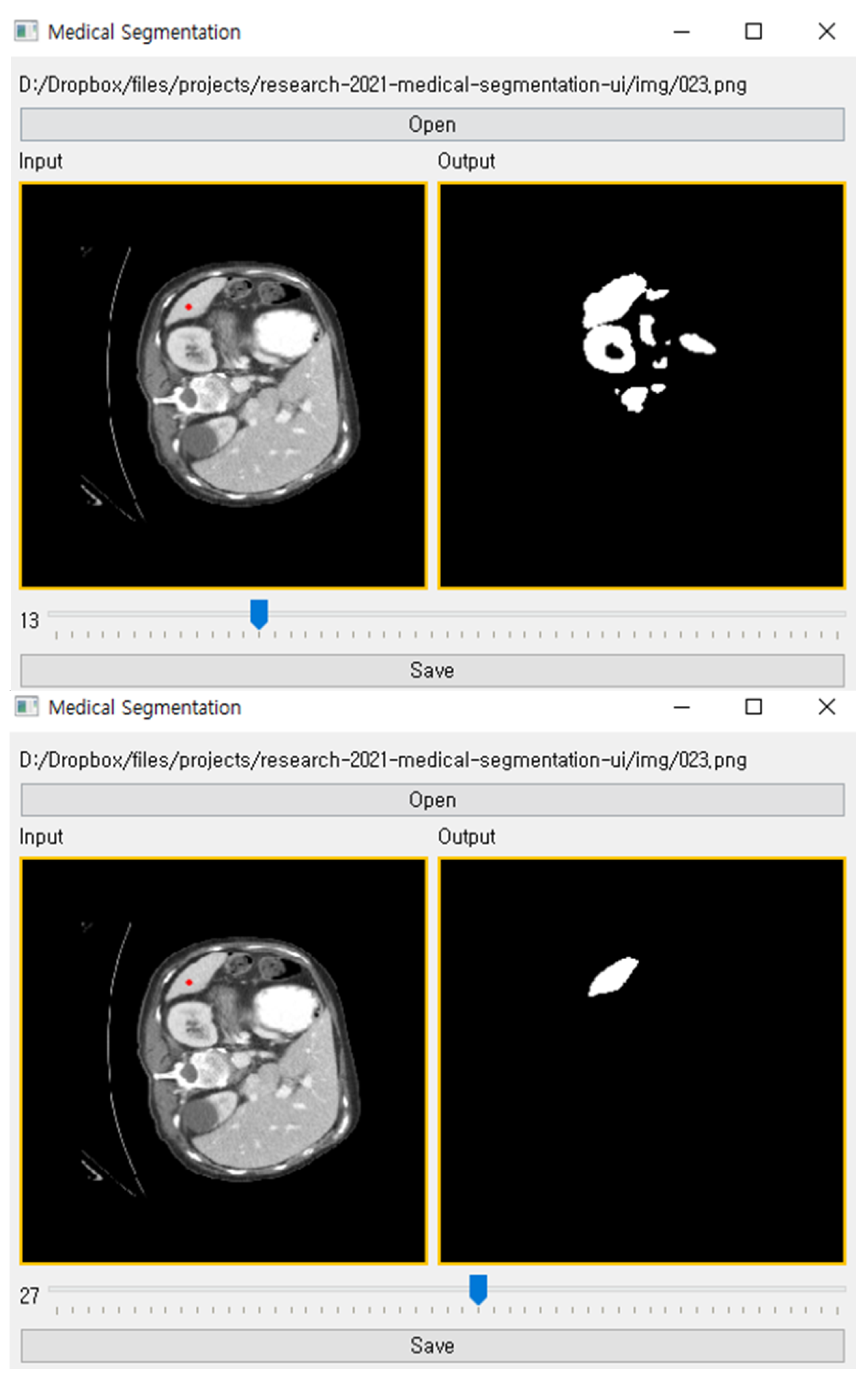
After training the proposed method with a little training data, a user can perform organ segmentation on a CT image. Figure 3 shows our tool in use. It contains the input CT image, anchor pixels entered by a user, threshold value, and segmented target organ image. A user can create labels using our tool as following order:

Figure 3. The user interface of our tool for reconstructing a segmentation label from a few anchor pixels. The upper figure shows the segmentation result when the threshold is 18. The lower figure is same as upper figure except for threshold value (which is 28).

• Open a CT image to perform segmentation;
• Select the target organ in category;
• Pick anchor pixels on the target organ. Once anchor pixels are picked, proposed model computes kernel density for all pixels;
• Extract the segmentation label by filtering the density that is higher than a threshold value.

To infer segmentation from a kernel density, a threshold value determines the lower density bound of the segmentation label. The suitable threshold value can be different for each organ since each organ has various sizes and shapes in a CT image. In order to enable adjusting the threshold value, we added a slider in the bottom of the interface, as illustrated Figure 3. Through the slider, a user can manipulate the threshold to generate a proper segmentation label on input CT image.

4. Performance Tests

This section explains the experiment environment and results. This work was implemented with PyTorch [26], and the user interface was built with PyQT. When implementing evaluation metrics, we utilized the MONAI (https://monai.io/, accessed on 1 September 2021) library. The model training and inference are conducted on an Ubuntu machine with NVIDIA GTX 1080 Ti GPU installed. We visualized our experiments using the Weight & Bias [27] tool.

4.1. Performance Evaluation with Varying Threshold

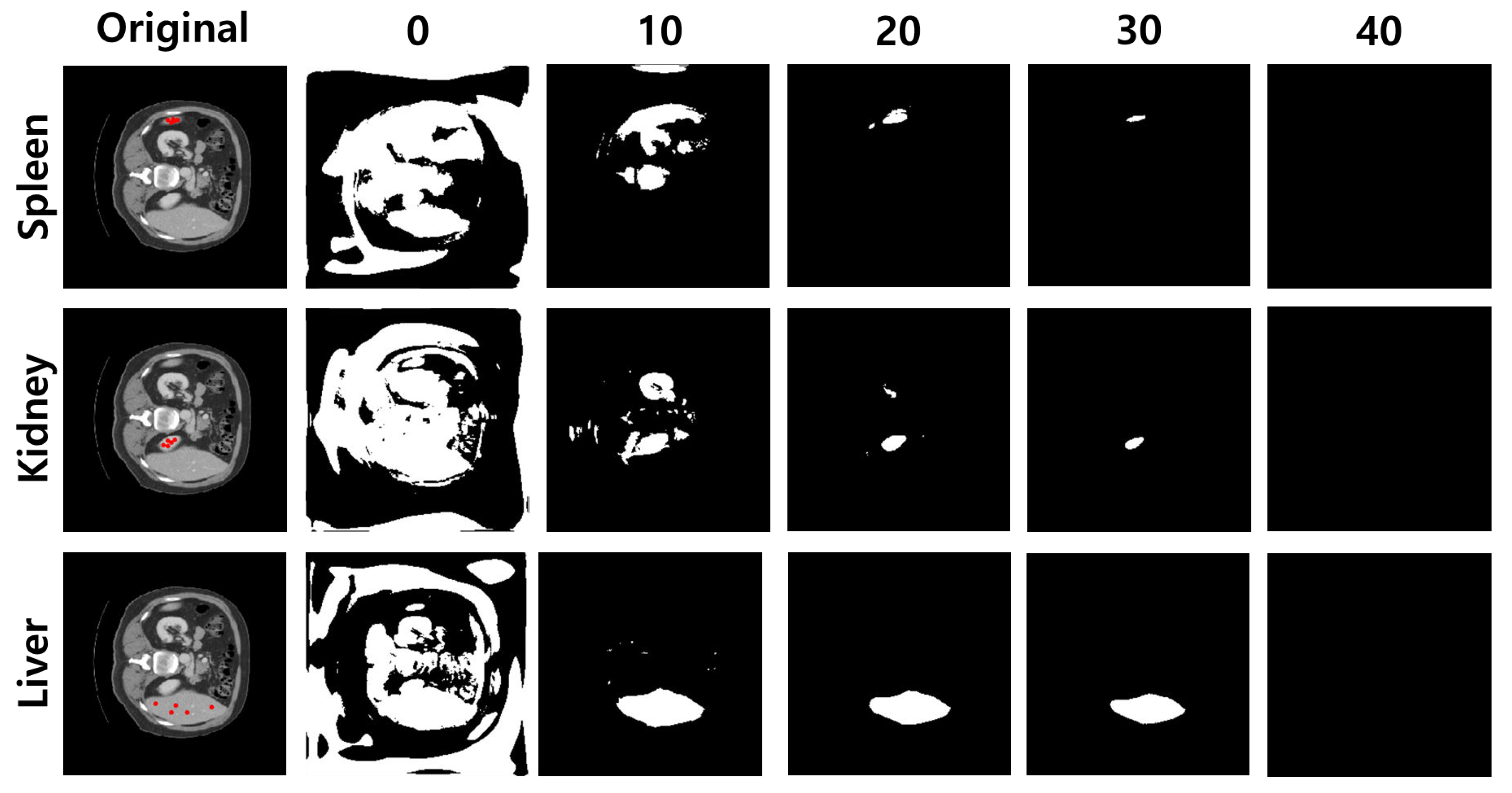
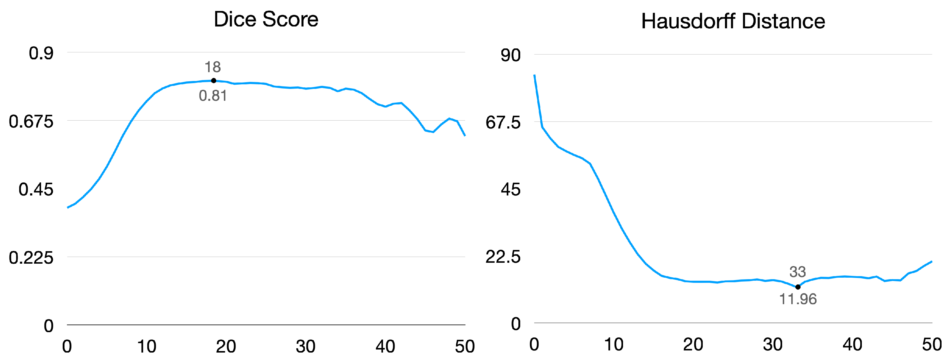
A threshold value is a hyperparameter to draw segmentation results from a kernel density. Because the quality of the result depends on the threshold, the appropriate threshold value is required. To show the influence of the threshold value, we visualize segmentation images and measure the metrics of the segmentation, varying the threshold values from 0 to 50.

Given the anchor pixels and threshold value, Figure 4 illustrates segmentation images of each target organ. As a result, the lower threshold captures the region roughly, and the higher value shrinks the area to narrow. The dice score and Hausdorff distance are for measuring segmentation performance. As shown in Figure 5, the dice score reached 0.81 when the threshold value was 18, and the Hausdorff distance achieved a minimum distance of 11.96 when the threshold value was 33.

Figure 4. Segmentation Examples by Threshold. Each row represents each organ. First column shows original CT images, and from the second to sixth columns, the segmentation generated from 5 anchor pixels is shown. We visualize segmentation by different thresholds.

Figure 5. Dice score and Hausdorff distance by varying thresholds. Left graph demonstrates change in dice score by changing thresholds. Right graph shows Hausdorff distance by varying thresholds.

We analyzed that the dice score tends to be high when there is an intersection region between the predicted region and ground truth, even though a non-organ region is captured. In contrast, the Hausdorff distance tends to be low when the boundary of the predicted region is close to the ground truth. Our experiments focus more on capturing all regions of the target organ than predicting its boundary. As a result, we fix the threshold value as 18 in the following experiments.

4.2. Performance Evaluation with Varying the Number of Anchor Pixels

The proposed model requires a few anchor pixels on the organ to be segmented. The performance of the model can be affected by the number of anchor pixels picked by the user. The anchors are sampled randomly in the ground truth for convenience in the experiments. We tried to find out the best number of anchor pixels for our method.

As shown in Table 1, we measured the dice score and Hausdorff distance of our model according to the number of anchor pixels for the proposed method. The dice score is the lowest when using only one anchor pixel for each organ, and the dice score when using two or more anchor pixels is almost similar. However, the Hausdorff distance instead increases because other organs with similar textures to the target organ are often segmented.

Table 1. Dice score and Hausdorff distance by changing the number of anchors.

	Number of Anchor Pixels per Organs
Model	1	2	3	4	5
DICE SCORE	0.717	0.752	0.761	0.762	0.759
Hausdorff Distance	29.155	14.956	18.748	20.433	17.951

Figure 6 shows how the number of anchor pixels affects the segmentation reconstructed from anchor pixels. As those figures illustrate, our model can find a segmentation region with a missing area when we pick only one anchor pixel. However, as the number of anchor pixels increases, the proposed method captured a more accurate region.

Figure 6. Case study to see how the generated segmentation is changed by a changing number of anchor pixels. The first and third columns are original CT images with some anchor pixels (red points). The second and fourth columns are generated segmentation using given anchor pixels.

Generally, more anchor pixels give better segmentation than fewer anchor pixels. However, we could find some exceptional cases that fewer anchor pixels show better performance. We analyzed that the position of anchor pixels also affects the performance. For instance, even if we have only one anchor pixel, the segmentation prediction is more accurate when the anchor pixel exists around the center of the organ. If we have more than one anchor pixel, but they are in the boundary, our model tends to capture only a part of the region. Since we automated the process of picking anchor pixels by randomly sampling them from pixels of the organ, the case that some anchor pixels cover the same region or exist in the boundary region frequently occurred.

4.3. Tests on Segmentation Accuracy

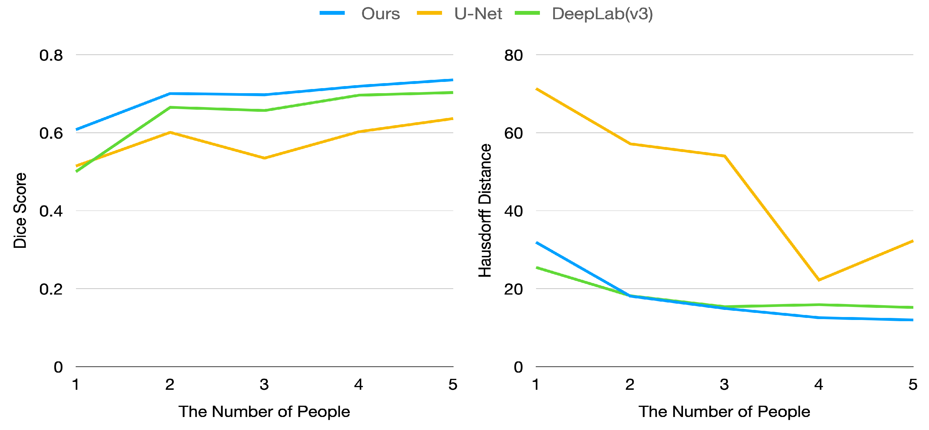
In our case, we focus on making the model show acceptable performance when a few labeled data are given. To verify the performance of our model, we measured the evaluation metrics by varying the number of training data. The x-axis of Figure 7 represents the number of people extracted from labeled images. In this experiment, we used only five CT images per person.

Figure 7. Dice score and Hausdorff distance by changing size of training data (number of people in training data).

Figure 7 shows the dice score and Hausdorff distance of the proposed model and baseline models. As illustrated in Figure 7, our model is superior to baseline models in terms of dice score. In particular, our model achieved a 0.6 dice score with training data of only one person, whereas baseline models achieved only about 0.5 dice score.

However, our model has a higher Hausdorff distance than DeepLab-V3 because segmentation generated by DeepLab-V3 is rarely scattered. In contrast, our method can generate segmentation with some scattered points since our approach exploits the density computed using visual similarity between pixels. If there are points that have similar features with anchor pixels, these points can be classified as part of the target organ, even if these pixels are apart from the target organ (this circumstance can also be found in Figure 4). This drawback can be relieved by carefully picking anchor pixels and thresholding.

We also compared our model with other semi-automatic algorithms, such as the active contour algorithm and the watershed algorithm. We exploited the true segmentation label to construct informative seed for the watershed algorithm. However, we found that these algorithms poorly detected the region of organs and achieved a dice score too low (0.04 and 0.07, respectively).

4.4. Ablation Study

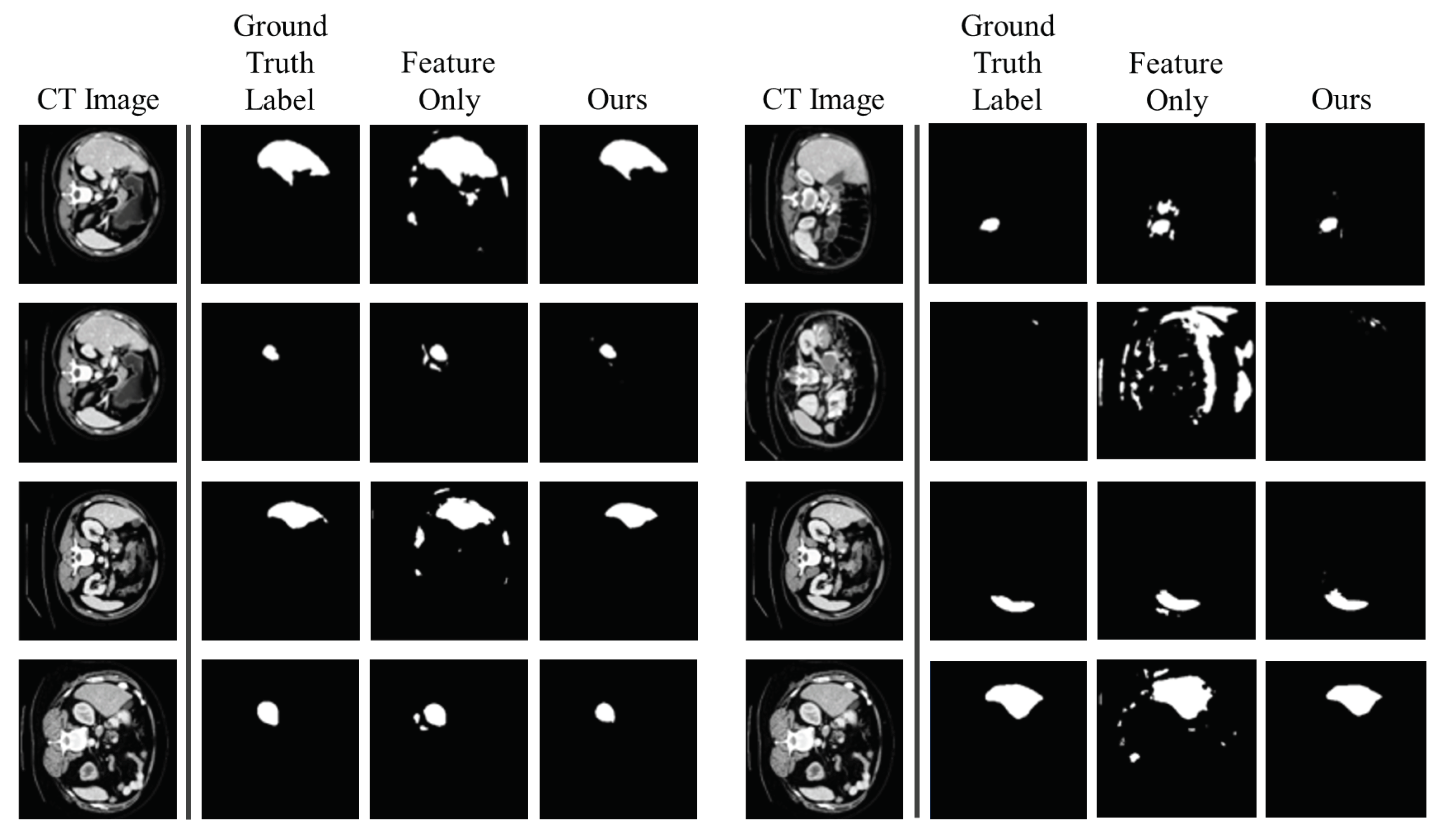
This experiment explains the ablation study explain why these two kernel modules are necessary. As shown in Table 2, if we have only the Gaussian kernel density, the performance becomes lower than any other models in terms of both dice score and Hausdorff distance. At this point, we adjusted the threshold to 0.5 since the Gaussian kernel density generally has a small value. The threshold value of 0.5 is selected by the experiment to perform better. The performance drop is not huge when we take only the feature similarity kernel density (feature-only model). However, as illustrated in Figure 8, the feature-only model generates more scattered segmentation than ours. Therefore, utilizing the Gaussian kernel density to generate segmentation labels is necessary in order to avoid scattering, although the feature-only model has a tiny performance drop.

Table 2. Ablation study for kernels.

Gaussian Kernel	Feature Kernel	Dice Score	Hausdorff Distance
O	O	0.7590	23.31
O	X	0.3795	31.08
X	O	0.7370	23.85

Figure 8. Ablation Study: Importance of the Gaussian Kernel. The first and fifth columns are CT images. The second and sixth columns are ground truth segmentation labels. The third and seventh columns are predictions generated by the model without the Gaussian kernel. The fourth and last columns are predictions generated by our model (Gaussian kernel + feature similarity kernel).

5. Conclusions

In this work, we proposed a tool that allows users to obtain segmentation labels by picking a few pixel points on the organ. The tool cannot segment without giving a pixel point but has the advantage that learning requires less labeled data than previous studies and makes data collection easier. This tool calculates the kernel density for all pixels, finds areas equal to or greater than a specific threshold value, and demonstrates its performance through experiments. However, the proposed method has a constraint that some non-target regions nearby a target organ could be classified as the same organ when the pixels have similar visual characteristics to a target organ. Furthermore, if an organ has various textures or multiple regions, our algorithm may miss some regions of the organ. Even though these constraints can be mitigated by carefully adjusting the threshold value, we should improve our algorithm in future work.

References

- Pham, D.L.; Xu, C.; Prince, J.L. Current methods in medical image segmentation. Annu. Rev. Biomed. Eng. 2000, 2, 315–337. [Google Scholar] [CrossRef]
- Ciresan, D.; Giusti, A.; Gambardella, L.; Schmidhuber, J. Deep neural networks segment neuronal membranes in electron microscopy images. Adv. Neural Inf. Process. Syst. 2012, 25, 2843–2851. [Google Scholar]
- Havaei, M.; Davy, A.; Warde-Farley, D.; Biard, A.; Courville, A.; Bengio, Y.; Pal, C.; Jodoin, P.M.; Larochelle, H. Brain tumor segmentation with deep neural networks. Med. Image Anal. 2017, 35, 18–31. [Google Scholar] [CrossRef] [PubMed] [Green Version]
- Zhang, W.; Li, R.; Deng, H.; Wang, L.; Lin, W.; Ji, S.; Shen, D. Deep convolutional neural networks for multi-modality isointense infant brain image segmentation. NeuroImage 2015, 108, 214–224. [Google Scholar] [CrossRef] [PubMed] [Green Version]
- Roth, H.R.; Farag, A.; Lu, L.; Turkbey, E.B.; Summers, R.M. Deep convolutional networks for pancreas segmentation in CT imaging. In Proceedings of the Medical Imaging 2015: Image Processing; International Society for Optics and Photonics: San Diego, CA, USA, 2015; Volume 9413, p. 94131G. [Google Scholar]
- Tajbakhsh, N.; Shin, J.Y.; Gurudu, S.R.; Hurst, R.T.; Kendall, C.B.; Gotway, M.B.; Liang, J. Convolutional neural networks for medical image analysis: Full training or fine tuning? IEEE Trans. Med. Imaging 2016, 35, 1299–1312. [Google Scholar] [CrossRef] [PubMed] [Green Version]
- Ronneberger, O.; Fischer, P.; Brox, T. U-Net: Convolutional Networks for Biomedical Image Segmentation; MICCAI: Strasbourg, France, 2015. [Google Scholar]
- Liu, Y.; Lei, Y.; Fu, Y.; Wang, T.; Tang, X.; Jiang, X.; Curran, W.J.; Liu, T.; Patel, P.R.; Yang, X. CT-based Multi-organ Segmentation using a 3D Self-attention U-Net Network for Pancreatic Radiotherapy. Med. Phys. 2020, 47, 4316–4324. [Google Scholar] [CrossRef] [PubMed]
- Li, S.; Tso, G.K.F.; He, K. Bottleneck feature supervised U-Net for pixel-wise liver and tumor segmentation. Expert Syst. Appl. 2020, 145, 113131. [Google Scholar] [CrossRef]
- Wang, L.; Wang, B.; Xu, Z. Tumor Segmentation Based on Deeply Supervised Multi-Scale U-Net. In Proceedings of the 2019 IEEE International Conference on Bioinformatics and Biomedicine (BIBM), San Diego, CA, USA, 18–21 November 2019; pp. 746–749. [Google Scholar]
- Liu, Z.; Liu, X.; Xiao, B.; Wang, S.; Miao, Z.; Sun, Y.; Zhang, F. Segmentation of organs-at-risk in cervical cancer CT images with a convolutional neural network. Phys. Med. PM Int. J. Devoted Appl. Phys. Med. Biol. Off. J. Ital. Assoc. Biomed. Phys. 2020, 69, 184–191. [Google Scholar] [CrossRef] [PubMed] [Green Version]
- Liu, Z.; Song, Y.Q.; Sheng, V.S.; Wang, L.; Jiang, R.; Zhang, X.; Yuan, D. Liver CT sequence segmentation based with improved U-Net and graph cut. Expert Syst. Appl. 2019, 126, 54–63. [Google Scholar] [CrossRef]
- Gao, Y.; Zhou, M.; Metaxas, D.N. UTNet: A Hybrid Transformer Architecture for Medical Image Segmentation. arXiv 2021, arXiv:2107.00781. [Google Scholar]
- Wang, Z.; Zou, Y.; Liu, P.X. Hybrid dilation and attention residual U-Net for medical image segmentation. Comput. Biol. Med. 2021, 134, 104449. [Google Scholar] [CrossRef] [PubMed]
- Li, Y.; Wang, Z.; Yin, L.; Zhu, Z.; Qi, G.; Liu, Y. X-Net: A dual encoding–decoding method in medical image segmentation. Vis. Comput. 2021, 1–11. [Google Scholar] [CrossRef]
- Hatamizadeh, A.; Yang, D.; Roth, H.R.; Xu, D. UNETR: Transformers for 3D Medical Image Segmentation. arXiv 2021, arXiv:2103.10504. [Google Scholar]
- Cao, H.; Wang, Y.; Chen, J.; Jiang, D.; Zhang, X.; Tian, Q.; Wang, M. Swin-Unet: Unet-like Pure Transformer for Medical Image Segmentation. arXiv 2021, arXiv:2105.05537. [Google Scholar]
- Liu, Z.; Lin, Y.; Cao, Y.; Hu, H.; Wei, Y.; Zhang, Z.; Lin, S.; Guo, B. Swin transformer: Hierarchical vision transformer using shifted windows. arXiv 2021, arXiv:2103.14030. [Google Scholar]
- Girum, K.B.; Créhange, G.; Hussain, R.; Lalande, A. Fast interactive medical image segmentation with weakly supervised deep learning method. Int. J. Comput. Assist. Radiol. Surg. 2020, 15, 1437–1444. [Google Scholar] [CrossRef]
- Wang, G.; Li, W.; Zuluaga, M.A.; Pratt, R.; Patel, P.A.; Aertsen, M.; Doel, T.; David, A.L.; Deprest, J.A.; Ourselin, S.; et al. Interactive Medical Image Segmentation Using Deep Learning with Image-Specific Fine Tuning. IEEE Trans. Med. Imaging 2018, 37, 1562–1573. [Google Scholar] [CrossRef]
- Weng, G.; Dong, B.; Lei, Y. A level set method based on additive bias correction for image segmentation. Expert Syst. Appl. 2021, 185, 115633. [Google Scholar] [CrossRef]
- Landman, B.; Xu, Z.; Igelsias, J.E.; Styner, M.; Langerak, T.; Klein, A. MICCAI multi-atlas labeling beyond the cranial vault–workshop and challenge. In Proceedings of the MICCAI: Multi-Atlas Labeling Beyond Cranial Vault-Workshop Challenge, Munich, Germany, 5–9 October 2015. [Google Scholar]
- Kingma, D.P.; Ba, J. Adam: A Method for Stochastic Optimization. CoRR 2015. CoRR:abs/1412.6980. [Google Scholar]
- Gutmann, M.U.; Hyvärinen, A. Noise-Contrastive Estimation: A New Estimation Principle for Unnormalized Statistical Models. In Proceedings of the AISTATS, Sardinia, Italy, 13–15 May 2010. [Google Scholar]
- van den Oord, A.; Li, Y.; Vinyals, O. Representation Learning with Contrastive Predictive Coding. arXiv 2018, arXiv:1807.03748. [Google Scholar]
- Paszke, A.; Gross, S.; Massa, F.; Lerer, A.; Bradbury, J.; Chanan, G.; Killeen, T.; Lin, Z.; Gimelshein, N.; Antiga, L.; et al. PyTorch: An Imperative Style, High-Performance Deep Learning Library. In Proceedings of the 2019 NeurIPS, Vancouver, BC, Canada, 8–14 December 2019. [Google Scholar]
- Biewald, L. Experiment Tracking with Weights and Biases. 2020. Available online: wandb.com (accessed on 1 October 2021).