Article

Analysis of Some Power Quality Parameters at the Points of Common Coupling of Photovoltaic Plants Based on Data Measured by Inverters

by
Isabel Santiago
*,
Javier García-Quintero
,
Gonzalo Mengibar-Ariza
,
David Trillo-Montero
,
Rafael J. Real-Calvo
and
Miguel Gonzalez-Redondo
Departamento de Ingeniería Electrónica y de Computadores, Campus de Rabanales, Universidad de Córdoba, 14071 Córdoba, Spain
*
Author to whom correspondence should be addressed.
Appl. Sci. 2022, 12(3), 1138; https://doi.org/10.3390/app12031138
Submission received: 16 December 2021 / Revised: 16 January 2022 / Accepted: 18 January 2022 / Published: 21 January 2022

Abstract

:
With the increasing implementation of renewable energies, the impact that this type of installation can have on the electricity supply grid is of great importance. In this context, the aim of this work is to analyse how the production and injection of electricity generated by a series of small photovoltaic (PV) installations influence some parameters of the electricity grid in the low-voltage (LV) distribution networks to which they are connected, by analysing the basic data provided by the inverters of these installations. The presence of a slight rise in the grid voltage values in the Point of Common Coupling (PCC) as the production of the PV plants increases has been verified, with maximum slopes between 0.95 and 0.00027 V/kW, but which do not result in voltage values close to the limits set by the regulations. In addition to assessing this impact, the results obtained made it possible to determine the hosting capacity that the networks into which these installations inject their energy would have for this type of installation so as not to have a detrimental effect on the voltage values of the grid. The possible influence of the production of PV installations on the voltage imbalance between phases or on the frequency of the grid has also been analysed in this work. Although the values recorded by the inverters have limitations in their measurements that do not make them valid for assessing events such as the presence of harmonics or flickers, they do allow a first analysis to be made of the influence of PV plant production on some grid parameters, without the need to incorporate additional measurement systems in these renewable installations. However, it is important to be aware of the limitations of the measurements of this equipment and, as far as possible, to choose inverter models that carry out this type of measurement as completely as possible.

1. Introduction

Over the course of time and thanks to technological development, renewable energies have experienced great growth in recent years, and everything indicates that this increase will continue in the future [1], reducing dependence on fossil fuels and allowing a closer approach to the environmental objectives set by different countries and organisations [2]. With more than 700 GW of capacity globally, solar PV was the most installed renewable energy source in recent years. It is now considered the fastest growing power generation source, representing 48% of the world’s clean energy capacity installed and connected to the grid in 2020; and the forecast is that in the next few years, the world’s solar generation would reach the terawatt production capacity level [3,4].
One of the reasons for this increase in PV power capacity has been the reduction in PV prices over the last few years, a reduction which is still continuing [5]. The cost of generating electricity from distributed solar PV systems is already below retail electricity prices in most countries. The International Energy Agency (IEA) forecasts that these costs will decline by a further 15 to 35% by 2024, making the technology even more attractive and stimulating its adoption worldwide [3,6]. Improvements in module performance, as well as the simplicity and reliability of such installations, have also contributed to their widespread use. In addition, the increasing penetration of this technology will reduce the dependence on imported energy resources in many countries [7].
A significant percentage of the installed solar energy corresponds to distributed PV systems in homes, commercial buildings and industry [8,9]. The capacity of this type of installation has almost tripled since 2014, transforming the way electricity is generated and consumed; and it is expected that the distributed PV accounts for almost half of the growth in the overall solar PV market through 2024 [6]. These figures could even increase in the future with the application of innovative solar photovoltaic roof panels to better integrate generation into the construction of buildings [10].
However, LV distribution electricity systems were designed as passive networks in a radial style, and were not meant to accommodate distributed generation, so the integration of renewable energy systems (RESs) in electricity networks may cause some issues and impacts on the power quality, protection coordination and operation of distribution feeders that need to be carefully analysed [11,12].
PV generation is highly variable, which is one of the main drawback of the large-scale application of PV in distribution networks [13,14]. The irregular nature of the solar radiation, often caused by the rapid pass of different types of clouds or by the presence of shadows [15], means that the output of this type of installation presents intermittency or random fluctuations [16]. The transient atmospheric changes that affect the variability of renewable production has a stochastic character in general with different conditions of duration, frequency, magnitude and shape [17]. The duration of irradiance transitions may vary from a few seconds up to several minutes, and the number of transitions in a day can be as many as 500, the highest transition rates taking place around noon [18]. These irradiance fluctuations can lead to situations where the inverters are not able to follow the global maximum power point (MPP) causing extra losses, and partial shading of PV generators also causes mismatch losses [15,18].
Moreover, this fluctuated dynamic of electricity production, which mainly affects small PV installations due to their not exhibiting the smoothing effect present in larger ones [19], may have its consequences in customers, residential and industrials, and even in the own network. It may create a problem in balancing demand and production [11], provoking the presence of reverse power flow, which may lead to the occurrence of supply quality problems such as voltage variations and imbalance, current and voltage harmonic distortion [20,21], grid islanding protection, voltage flickers [22] and other power quality issues [23,24,25]. This can also produce stress and increased wear on voltage regulation devices and distribution transformers, which can reduce their lifespan or even cause them to malfunction [12]. In addition, the frequency variations that occur in the grid due to the change of the connected loads can be aggravated if there are fluctuations in the PV production [13]. The severity of all these issues depends on the penetration level of PV, on the configuration of distribution systems and on the location of PV in them.
Therefore, one of the main challenges that need to be overcome to speed up the deployment of this type of renewable sources is their correct integration in energy networks, needed to ensure that distributed PV’s growth is sustainable. As a result, there are numerous studies in the literature that review the potential impacts of distributed PV on the LV distribution grids [9,11,12,26] and they propose a variety of methods to mitigate the effects that might be produced on them, such as coordinated control strategies [7,27,28], distributed energy storage systems [8,13], geographical dispersion of distributed resources [13], active power curtailment [13], production forecasting [29], reactive power management [29,30] or improving electricity infrastructure [31].
A detailed analysis of the impact on the grid of PV plant operation would require a complete electrical signal measurement system, including harmonic distortion measurement with a network analyser [32]. Most of the PV installations currently in operation do not have this measurement system, especially small distributed installations. However, in most of these plants, the data recorded by the inverters during production and grid feed-in are available. Obviously, the parameters recorded by the inverters are not as complete as they should be. For example, with these data, it is not possible to analyse the waveform, nor to study how the inverters of the installations affect the emission of harmonics and interharmonics in the grid [33,34,35]. In addition, the main limitation is the sampling frequency with which the parameters are recorded by inverters, in many cases with sampling periods every 5 min or even longer. This is not enough to record many of the events that occur, such as the appearance of flickers caused by fluctuations in production due to the passage of clouds, which, as already indicated, is another of the problems associated with distributed renewable generation and which cannot be detected with this sampling frequency [13,22]. However, by using measurements of parameters such as nominal value of grid voltage and grid frequency recorded by the inverters to correctly synchronise the injection of generated power, it is possible to analyse and draw some conclusions about the possible influence of the production of this type of installations on these parameters that characterise the grid signal, to which the consumers of the electricity system are sensitive to a greater or lesser extent, and which are fundamental to the safe and economic operation of the electricity system [36].
In addition, some authors maintain that not all grid problems are a consequence of the presence of distributed generation sources, and it is even contemplated that the presence of PV installations in the distribution grid can be used to compensate for some of the supply quality problems present in the grid for other reasons [37,38]. For example, Miller et al. [39] have been able to verify in a study carried out in Australia that the imbalances they have detected in the grid are not a consequence of the presence of the PV installations analysed.
In this context, the main objective of this work was to carry out an analysis of the impact of the production of several PV installations connected to the grid in the south of Spain on some parameters that characterise the quality of the electrical signal in the grid, using data recorded by their inverters over a period of three years. The aim of this work was to determine the variation ranges of the voltage and frequency of the grid signal, comparing these values recorded by the inverters when the PV installations are in operation and injecting electricity into the grid, with those values measured when there is no production in the plants, thus analysing the probable correlation between the possible variations of these parameters with the injection of current into the grid by the PV installations.
Based on the results and data available, it was also possible to estimate the maximum power of PV installations that could be connected to these distribution lines without its impact causing the voltage of the grid to exceed the limits indicated by the current regulation. The study carried out in this work was applied to several PV installations, with the aim of comparing the hosting capacity of different distribution lines to which these installations inject their production, both in urban and rural areas. It was observed by some authors that this effect is more important in weak residential and rural grids with high series resistance [36]. Furthermore, with the analysis of the results, this work highlights which inverter characteristics are most suitable for correctly measuring these grid parameters to carry out this type of study.
The rest of the paper is organised as follows. Section 2 shows the characteristics of the PV installations in which the analysis of the data recorded by their inverters was carried out, describing the characteristics of the measured data. In Section 3, the results found are presented and discussed, and the main conclusions are shown in Section 4.

2. Materials and Methods

The study carried out in this work was based on the data monitored by the inverters in six PV installations connected to grid located in the south of Spain, in the province of Cordoba. The main characteristics of these installations are shown in Table 1. Figure 1 shows the geographical distribution of the plants. As they are small nominal power installations, they inject their production into LV distribution networks.
The data recorded in the different PV installations were provided by the company that installed them, Solar del Valle, SL, which is responsible for the operation and maintenance of these plants. The data acquisition system of the PV installations is integrated in their inverters. Inverters are connected via RS485 to a device called SunnyWebbox from the manufacturer SMA Solar Technology AG. It is a device with a central communication unit that continuously collects all the data from the inverters of each PV installation. The measurement data were transmitted via a GSM modem from remote locations where there was no telephone or ADSL connection, so they were read directly from a computer, and connected to the network, consuming between 4 and 12 W of power.
Inverters measure a series of parameters related to the production they receive from the PV panels associated with them, as well as related to the electricity they deliver to the grid and their operating status. They also measure some parameters necessary for their operational management, and for regulating the current to be injected, to correctly synchronise their production with the grid signal. The values of the AC power at inverter output (PAC), the AC current injected into the grid (IAC), the AC voltage in the grid phases (VAC) and the grid frequency (fgrid) measured by the inverters were used in this work. The maximum measurement error in the inverters, at a temperature of 25 °C, was ±1% for the grid voltage VAC, that of the injected power PAC was ±3%, that of the injected current IAC was ±2%, and that of the grid frequency fgrid was ±0.1% [40].
The data measured by the inverters were displayed every 5 min, and they correspond to an average value of each parameter in this time interval. For this work, the data that were recorded in the plants during a period of 3 years, from 1 January 2011 to 31 December 2013 were used, which are the data to which authors have been able to have access.
In order to manage the information of interest measured by inverters, organised in daily files, a software application called S·lar was used, previously developed by some of the authors of this work with the aim of organising in an automated way all the information contained in the files and storing it in a set of relational databases. The application reads all the data contained in the different files and dumps them into the different tables of the databases. Details of this application can be found in previous publications [41,42]. Once all the information has been stored, the S·lar application makes it possible to obtain, for each parameter recorded by each inverter, a matrix with the values of such parameter during the entire monitoring period. So, this application facilitated rapid access to the data of each parameter, for subsequent processing and analysis.
The matrices of the previously indicated parameters were the basis for the analysis of this work. For the three-year period, these matrices have a dimension of 1096 columns × 288 rows, which correspond respectively to the 1096 days of the three-year period analysed, and to the 288 records of each parameter that are registered every 5 min during the 24 h of each day. These matrices were analysed in an automated way using Matlab. For this purpose, a series of programs were developed that allow the reading and selective access to the data of the matrices, the calculation of parameters, their processing, and their graphic visualisation, thus facilitating the analysis and information extraction.

3. Results and Discussion

Based on the analysis of the above-mentioned data collected by the inverters of the installations, the results obtained in relation to the possible impact of the operation of the different PV plants on the voltage and frequency values of the power supply are shown below.

3.1. Grid Voltage Values Recorded at Each PV Installation during the Monitoring Period

Firstly, the grid voltage values VAC measured by the inverters during the entire monitoring period at the PCC of each PV installation were evaluated to assess their possible relationship with the injection of the electricity generated at each plant. Authors such as Chaudhary et al. [43] consider that the voltage rise issue is one of the most likely negative effect of the high PV penetration, or Ganghi et al. [9] have indicated that voltage violations to be the most important factor limiting PV penetration.
To start with this evaluation, all the records made by the inverters of both the grid voltage VAC and the current injected 
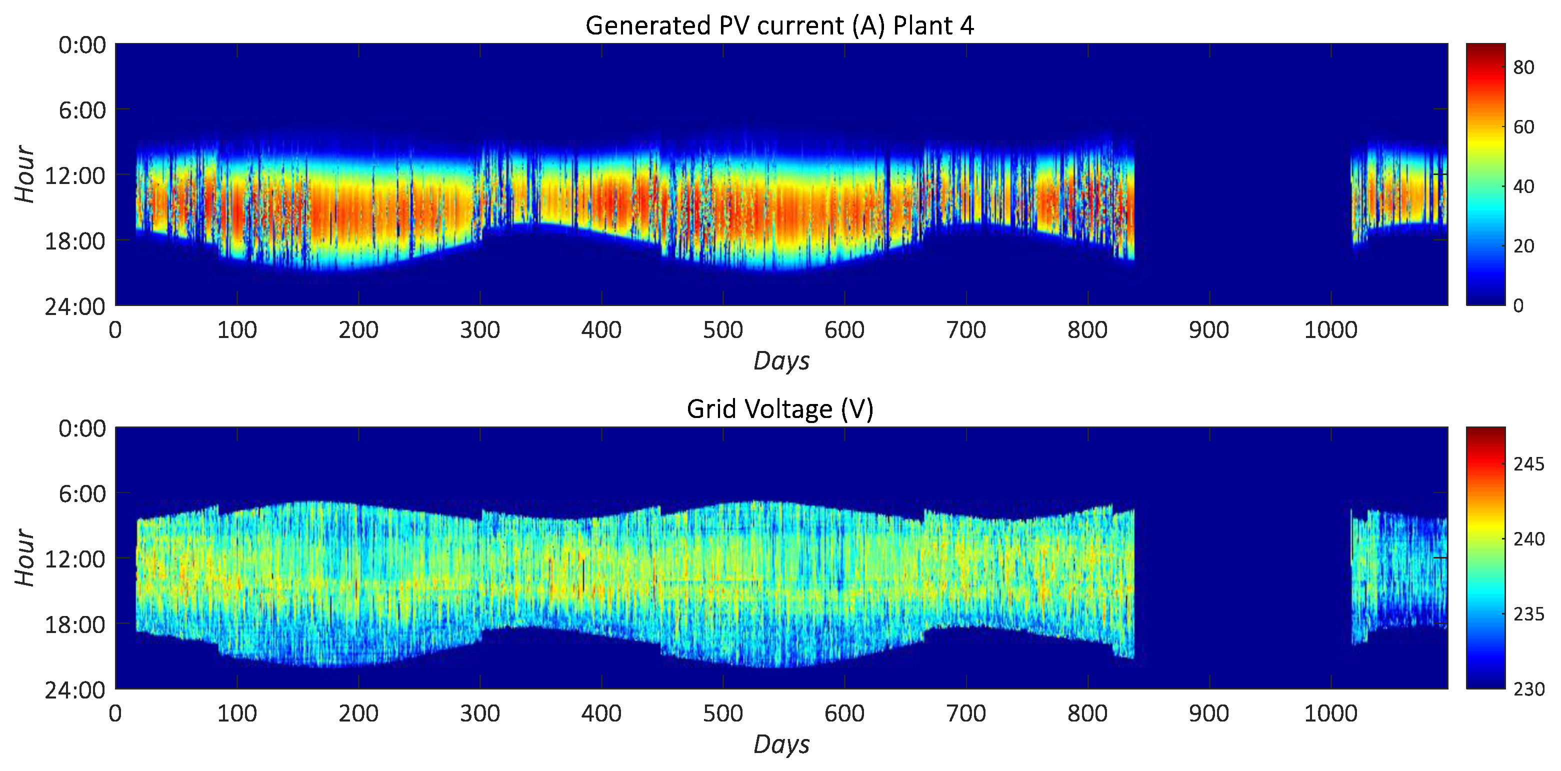
IAC by each installation have been represented in the form of colour maps. Figure 2 corresponds to one of the inverters of PV plant 1. With these graphs, it is possible to clearly visualise the values of these parameters over the period monitored in each of the installations.
The vertical axis of these figures shows the hour (corresponding to GMT+1 zone) at which the measurement was taken, and the horizontal axis shows the days of the time period analysed. Finally, the colours show in the upper graph the injected current, measured in A, and in the ground graph the VAC voltage, measured in V. As can be seen in the colour scale of these figures, the higher values of these parameters are represented in red; as they decrease, they turn yellow, then green, and finally, the lower values are shown in blue.
Figure 3 shows the distribution of the grid voltage values measured by an inverter in the PV plant 1 (already represented in Figure 2), but distinguishing two situations, one in which the plant’s production is injected into the grid, and the other in which the plant has no production and is not injecting energy into the grid.
In the same way that the measurements for PV plant 1 have been represented in Figure 2 and Figure 3, these two types of graphs (colour maps and histograms) have also been represented for the rest of the PV plants (Figure 4, Figure 5, Figure 6, Figure 7, Figure 8, Figure 9, Figure 10, Figure 11, Figure 12 and Figure 13).
In installations 1 and 2 (Figure 2 and Figure 4) the inverter model is monitoring the grid 24 h a day, so these grid voltage data are available all day long. In installations 3 to 6 (Figure 6, Figure 8, Figure 10 and Figure 12) the inverter model only registers the grid voltage values when the irradiance is above a certain threshold value, with which they are put into operation. Therefore, during the hours when there is no solar irradiance, the grid voltage values are not available. Therefore, in these graphs, these time instants were assigned the null value. Likewise, the voltage was assigned a null value in the periods of time when no data are available due to failures in the monitoring systems.
In installations 1 and 2, as they have three-phase inverters, the value of the current generated is evenly distributed in each of the three phases by this equipment. Although the inverter provides the voltage value in the three phases, in these figures, only the voltage value corresponding to one of the three phases was represented. The behaviour found in the other two phases was similar, as will be seen later.
In the rest of the installations studied, as they have single-phase inverters, each of them injects the current produced separately into only one of the phases (the number of inverters is a multiple of three to balance the injection of production into the grid). In this case, the inverter only provides the grid voltage values from the phase to which it is connected. For these installations, only the values corresponding to one of the inverters were shown in these graphs, and the results found for the other inverters connected to the other two phases were also similar.
In the graphs showing the electrical current produced in the different PV installations, it can be seen how its value increased in the central hours of the day, decreasing to zero at sunset and remaining at zero until sunrise the following day. It can be seen how the daily hours of electricity production were greater in the summer months than in the winter months due to the increase in the hours of sunshine at this time of year in this geographical location. It can also be observed that there were days in which there were fluctuations in production that corresponded to the passage of clouds, which means that solar radiation was in continuous variation throughout the day.
With respect to the graphs showing the grid voltage values, it can be observed that in general, the highest values were usually recorded in those hours when there was a higher production of electricity in the PV plants. Gandhi et al. [9] indicate that at high penetration of renewable PV installations, when PV generation exceeds the local electricity demand and causes reverse power flow, it can cause overvoltage problems.
The exception is found in installation 6 (Figure 12), located in a residential area within a city, where no such voltage increase was observed in the time instants when the PV plant output increased. This makes it clear that in this case the operation of the PV plant was not leading to an increase in grid voltage values. The influence of the installation’s production on the grid will be conditioned, in addition to the size of the plant, by the configuration of each grid, and by the characteristics of the loads connected to it. Therefore, performing this kind of analysis on the grid impact of all PV plants and being able to make use of inverter data to make a first estimation, without the need for additional measurements, can be very useful.
In addition to the increase in voltage that can be observed in 5 of the installations analysed in the central hours of the day, which are those of greatest PV production, it can be observed that at different times of the day, there were also increases in voltage values, even at night, which in this case were not associated with the operation of the PV plants. Therefore, as indicated by Miller et al. [39], it is clear that not all the deviations present in these grids can be attributed to the PV systems present in them.
As mentioned above, to complete the information displayed in Figure 2, Figure 4, Figure 6, Figure 8, Figure 10 and Figure 12, Figure 3, Figure 5, Figure 7, Figure 9, Figure 11 and 
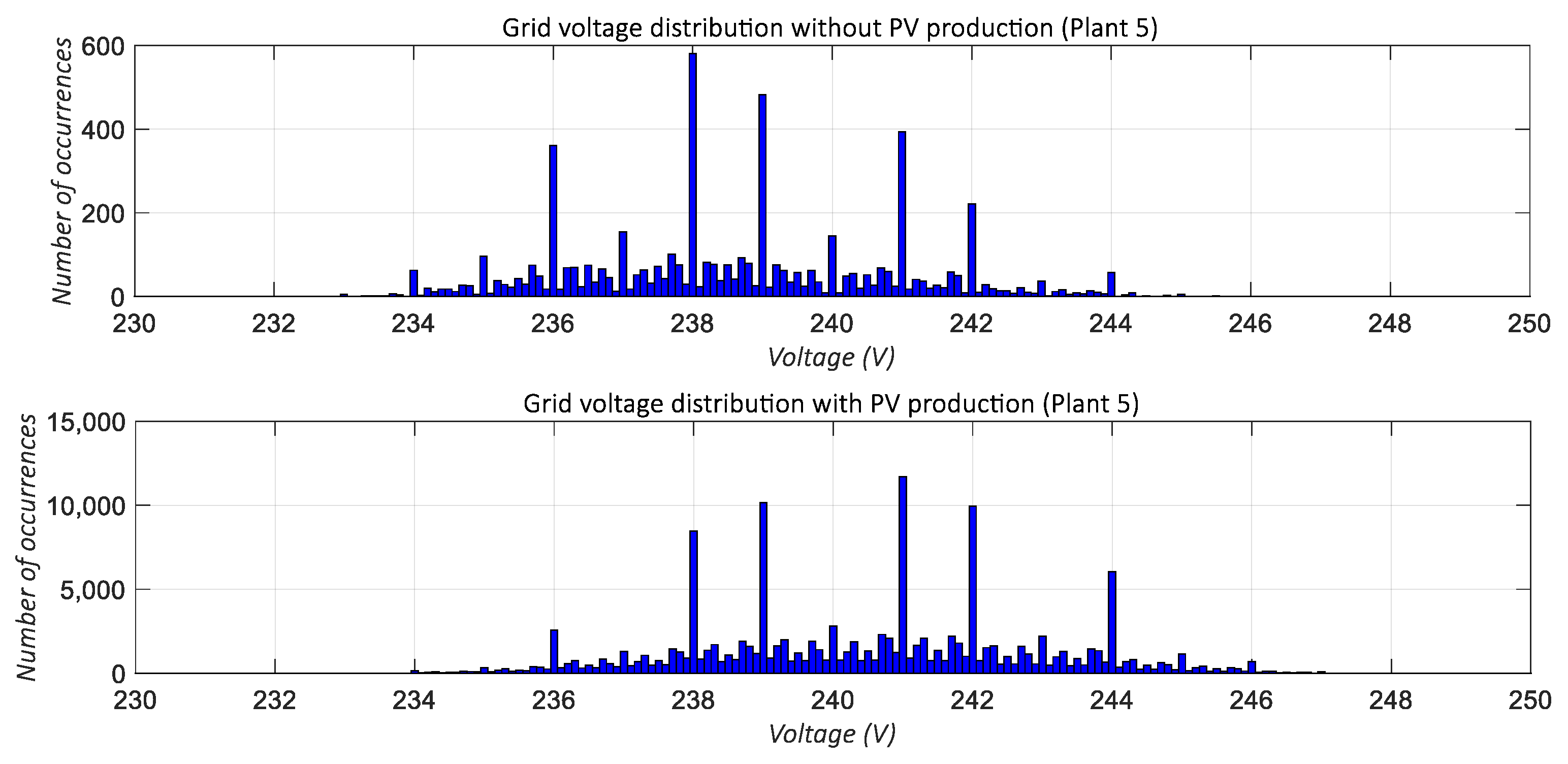
Figure 13 show the distribution of the grid voltage values measured by the inverters for each of the different PV installations, both when there is no power injection into the grid by the PV installation and when there is. In installations 3 to 6 (Figure 7, Figure 9, Figure 11 and Figure 13), the proportion of available voltage data corresponding to the situation where there is no current injection is much lower. Voltage values without PV production are only recorded in the early morning hours, when the inverter starts operating but is still trying to synchronise with the grid, and in the later hours of the day, when the inverter stops producing electricity until it shuts down. Since these inverter models are not measuring 24 h a day, the occurrences reflected in these graphs for the case of no plant production are much lower than in the case where there is PV production.
In Figure 3, Figure 5, Figure 7, Figure 9, Figure 11 and Figure 13, there was a general shift to the right and therefore an increase in voltage values when PV installations were feeding energy into the grid. The exception was, as seen previously, in installation 6 (Figure 13), where the voltage values hardly increased when the installation was producing electricity and injecting it into the grid. This is, as already indicated, a grid located within a city, and it is more resilient to the impact of the plant’s production, given that, as can be seen in Figure 12, the voltage values hardly increased during the hours when the PV installation was generating at its maximum.
It can be seen in Figure 7 (installation 3) and in Figure 11 and Figure 13 (installations 5 and 6) that certain grid voltage values appeared with a marked increase in probability with respect to the rest of the values, e.g., with a higher frequency of appearance, which suggests that in these cases, the behaviour of the statistical distribution was multimodal, unlike the rest of the installations where a monomodal trend can be seen. On the other hand, it can be seen in these cases (installations 3, 5 and 6) that the pattern of the statistical distribution of voltage values was maintained regardless of whether the PV plant injects energy, so it can be deduced that the origin of this behaviour was unrelated to the PV installations, indicating that the explanation for this behaviour was related exclusively to the state of the distribution network.
In this sense, the hypothesis considered to explain this multimodal behaviour is that the loads in the areas served by these installations could have a tendency towards some specific consumption values, more likely than others, which condition the values of the network voltage. Given that the histograms in Figure 7, Figure 11 and Figure 13 represent data frequency, it could be analysed how these voltage values were distributed over time by means of Figure 6, Figure 10 and Figure 12. In this way, it could be seen whether the most probable consumptions of the loads that cause this behaviour appear daily or at certain times of the year, which could be useful for the management of the electricity system itself. This detailed analysis was not carried out in the present work, but it will be carried out in future research.
Figure 14 plots the distribution of the grid voltage values recorded in the six PV plants, to show the data of all installations together. The non-zero VAC grid voltage data recorded by the inverters are plotted in box plots, showing the mean voltage for each installation (red line inside the box), the 75th percentile (the upper side of the box) and the 25th percentile (lower side of the box). The distance between these last two values is the inter quartile range. Since each PV installation injects into different distribution lines, the average voltage values in each of them were different, as they will depend on the specific point of the grid where they are located, and the distance from the transformer. The distribution of VAC values at each PCC was around 240 V in all the installations, except in the case of installation 3, where the values were lower, at around 220 V. The outliners that appear in Figure 14 (any values outside of the whiskers), show on the one hand, voltage values higher than the upper horizontal black lines, which correspond to the higher values recorded in each installation; and on the other hand, voltage values below the lower horizontal black lines are shown, which are point data that basically correspond to instants of time in which, after a fault, the inverter returns to operation but is not yet injecting energy into the grid. Therefore, these are not real grid voltage data but a consequence of how the inverter measures during reconnection after a fault period. If the grid voltage is outside the allowed range, the inverters have mechanisms to disconnect from the grid.
The highest grid voltage values were recorded in installation 2, which, as will be seen later, is where the greatest increase in voltage values occurs with the production of the PV plant; and despite the presence of this general increase in grid voltage values when there is power injection into the grid from the PV installations, only a couple of values recorded during the three years of operation in the different plants analysed are outside the ranges permitted by the regulations for this parameter.

3.2. Analysis of the Relationship between the Grid Voltage and the Power Generated by the Inverters

To further analyse the influence of PV plant production on the increase in grid voltage values, the correlation between the value of the grid voltage and the power generated in each PV installation was studied in detail. For this purpose, the value of the grid voltage VAC was represented on the Y-axis, and the value of the power injected into the grid at each time instant PAC was represented on the X-axis. Both parameters were measured by the inverters. Due to the large volume of data to be processed, these graphs were made for each of the months corresponding to the period monitored, and in each of the three different phases. Given the particularities of each installation, the following shows how this analysis was carried out in each one of them.
Plant 1. This installation consists of three three-phase inverters in which the power generated by each inverter is injected into the grid, distributing production evenly among the three phases. The inverters provide the voltage in each of the phases. Therefore, the VAC voltage value of each phase was represented with respect to PAC value resulted from the sum of the power produced by the three inverters divided by three due to the distribution between the three phases.
Plant 2. This installation has two three-phase inverters, of the same model as those in plant 1, in which the power generated in each inverter is divided by three to be injected in a balanced way in each of the phases. In this case, the VAC voltage value of each phase was represented with respect to the sum of the PAC power produced by the two inverters and in turn divided by three due to the distribution between the three phases.
Plant 3. This installation has six single-phase inverters distributed in such a way that they inject into each of the phases in groups of two. As they are single-phase inverters, each inverter only measures the voltage value corresponding to the phase to which it is connected. In this case, the VAC voltage of each phase recorded by one of the inverters connected to each phase was plotted against the sum of the PAC power generated by the two inverters connected to the same phase.
Plant 4. In the case of this installation, there are three single-phase inverters, each of which is connected to a different phase. The VAC voltage measured by each inverter on the phase into which it injects was therefore plotted against the PAC power generated by the same inverter.
Plant 5. In this case, this installation has 18 single-phase inverters that inject into each of the phases in groups of six inverters. The VAC measured by one of the inverters injecting on each phase was plotted against the sum of the PAC power generated by the six inverters injecting together on the same phase.
Plant 6. As in the case of plant 4, there are three single-phase inverters, each of which is connected to a different phase. The VAC voltage measured by each inverter was therefore plotted against the PAC power generated by the same inverter.
In these graphical representations of VAC versus PAC, the voltage limits established in the current standard were also included. The standard EN-50160 “Voltage characteristics of electricity supplied by public electricity networks”, indicates that the supply voltage variations must be 95% of time within the range 230 ± 10% at all supply terminals of the LV network [44]. Therefore, the lower and upper permissible levels for this parameter of the grid signal, corresponding respectively to the values 207–253 V, were represented in the figures in red.
In each of these graphical representations, the point cloud was fitted with a linear regression line, and this line was shown in green. In general, it was observed that the increase that takes place in the point cloud is correctly adjusted to a linear variation in many of the months analysed. However, there are some cases where the trend was not completely linear, and a good fit was not obtained given the low coefficient of determination (R2) values (shown below) obtained. However, the same type of adjustment was always used to be able to make a comparative analysis of the behaviour obtained during the whole monitoring period.
It should also be noted that these graphical representations only include voltage values recorded in those time instants in which the PV power production are different from zero. Voltage values registered when there was no injection of energy into the grid were excluded. For this purpose, it was necessary to filter out all those values recorded by the inverters in the time instants in which the inverters are operating, but there is still no injection of current into the grid. This filtering was necessary so that the calculation of the linear regression was not distorted by the null power values.
Figure 15 shows, as an example, monthly graphs for one of the phases in the different PV installations. The same trend found in the figures shown was also observed in the rest of the phases of the network. But the slope values were not constant, but changed in different ways over the period analysed, as will be seen later.
In the case of all PV installations, it can be observed that as the PV plant output that was injected into the grid increased, there was a slight increase in the grid voltage measured by the inverters, which shows, as previously seen, that the output of the plants was having some impact on the value of the grid voltage at that injection point. This behaviour was already found by Ronnberg et al. [36] for the case of PV installations located in Scandinavia.
It can be seen from the graphs that, since each PV installation injects its energy production at different points in the grid, the value of the Y-axis intercept, which would correspond to the value of the grid voltage without injection of production from the PV installation, was different for each installation and it depended on the PCC of each PV plant, as was also seen previously in Figure 14. It can also be seen in the graphs that for each value of PAC power injected in the installations, the voltage values observed had a variation range of between 5 and 10 V. In some cases, there may even be a greater variation range. This variation interval was maintained for all the power values, and it shows that the voltage values in the grid presented a previous variation that does not depend on the production of the plant and that can be considered unrelated to the operation of the PV installations.
The increase in grid voltage values that occurs with the increase in production of the PV plants is in addition to the variation that this parameter already has in the grid itself. However, the small values of the slopes found show that the increase is not very significant, and in general, with the production at each plant, it does not result in the grid voltage reaching values higher than those recommended by the regulations, given that the upper limit value was only reached in installation 2 very occasionally, as previously shown in Figure 14.
A comparison of graphs in Figure 15 shows that the lowest slope for the cases described was obtained in the case of installation 6, which reflects the lower increase in voltage already seen in Figure 12 and Figure 13. This shows a priori that the network into which this installation injects could be said to be the most resilient to the production of the PV installation of those analysed in this work, also taking into account that it is a PV installation with a small nominal power.
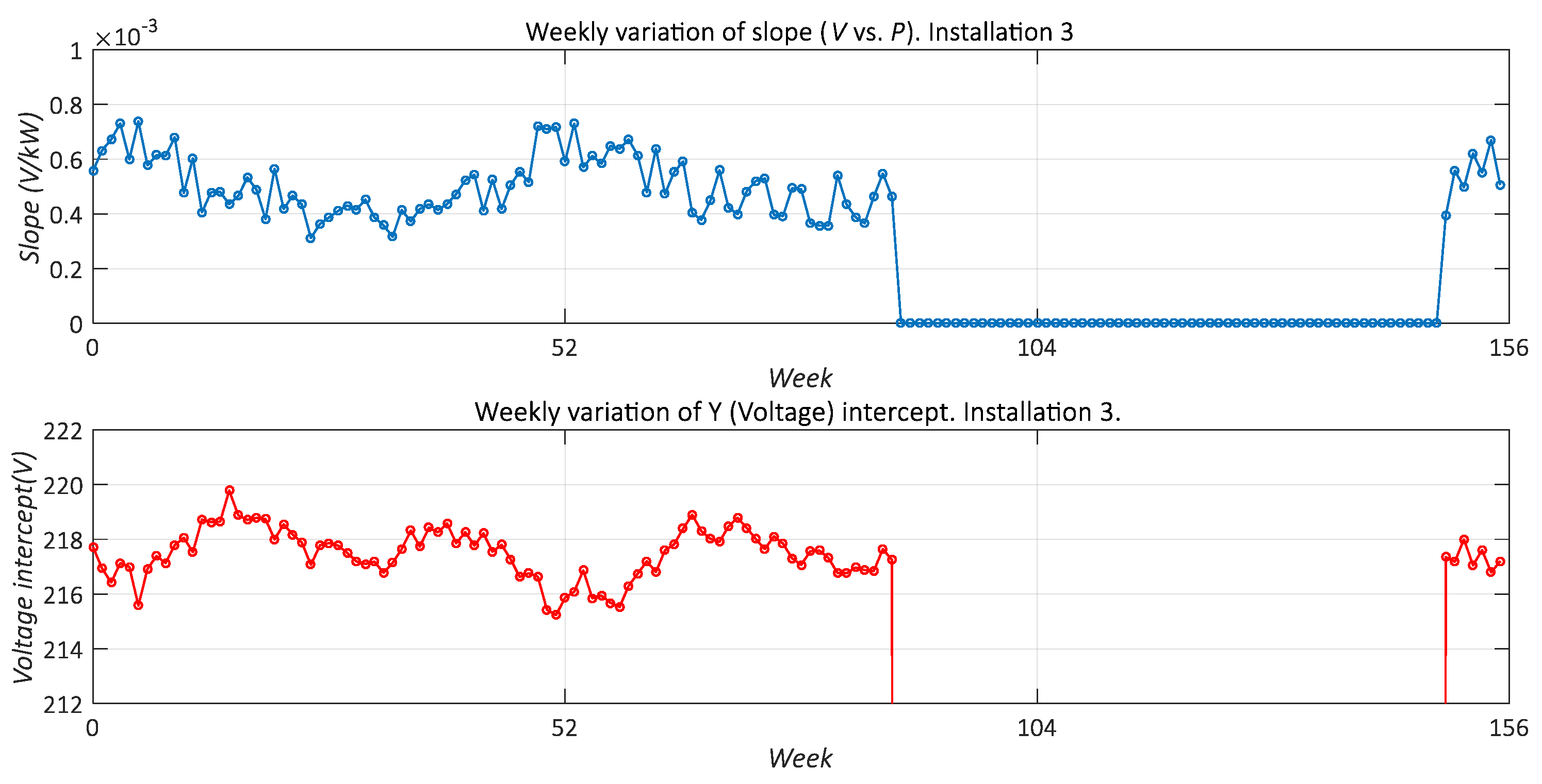
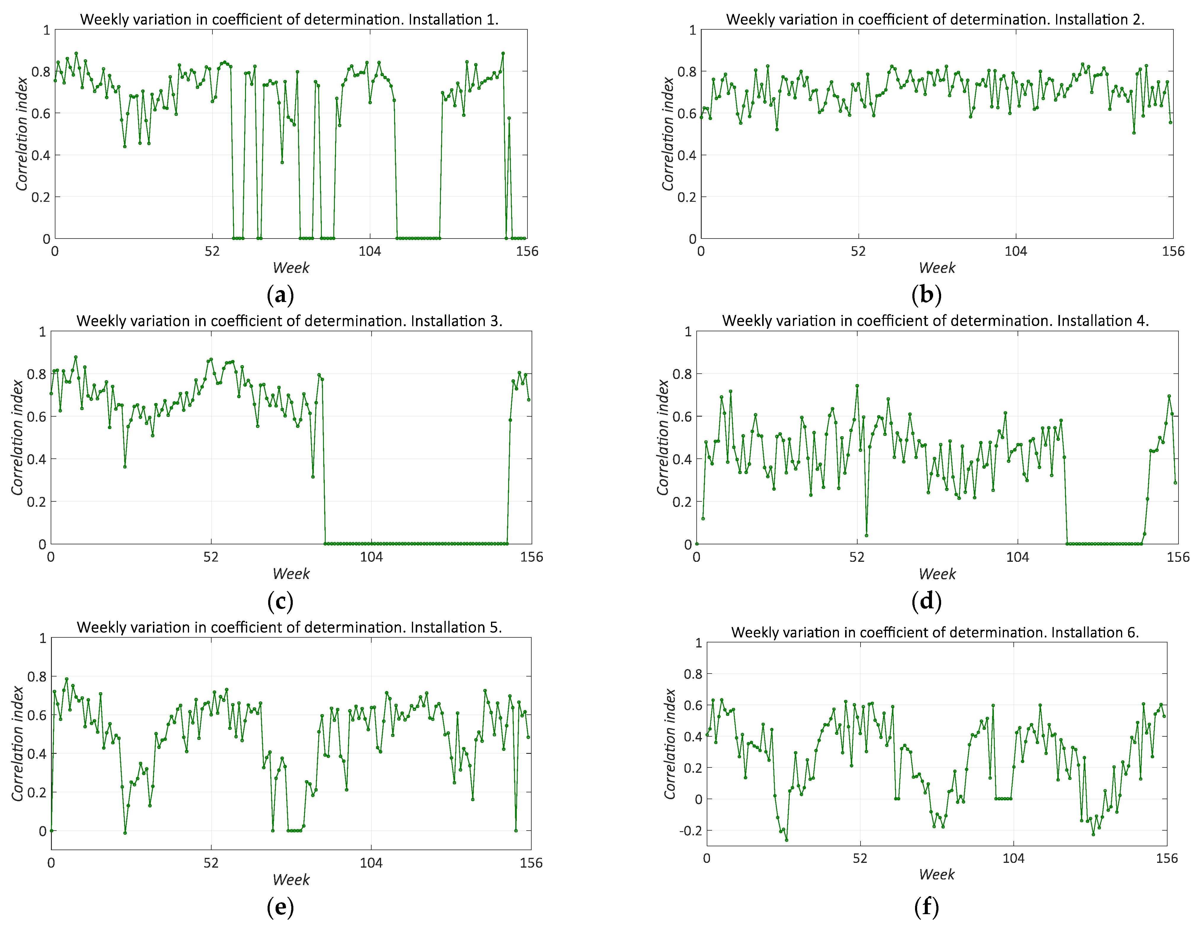
It was also found that the values of the slope of these graphs, as well as the Y-axis intercept, do not remain constant during all the months, but show a slight variation throughout the monitored period. For this reason, these slope values, together with the coefficient of determination of these linear fits, were calculated weekly for the entire monitored period, in order to analyse this variation.
Figure 16, Figure 17, Figure 18, Figure 19, Figure 20 and 
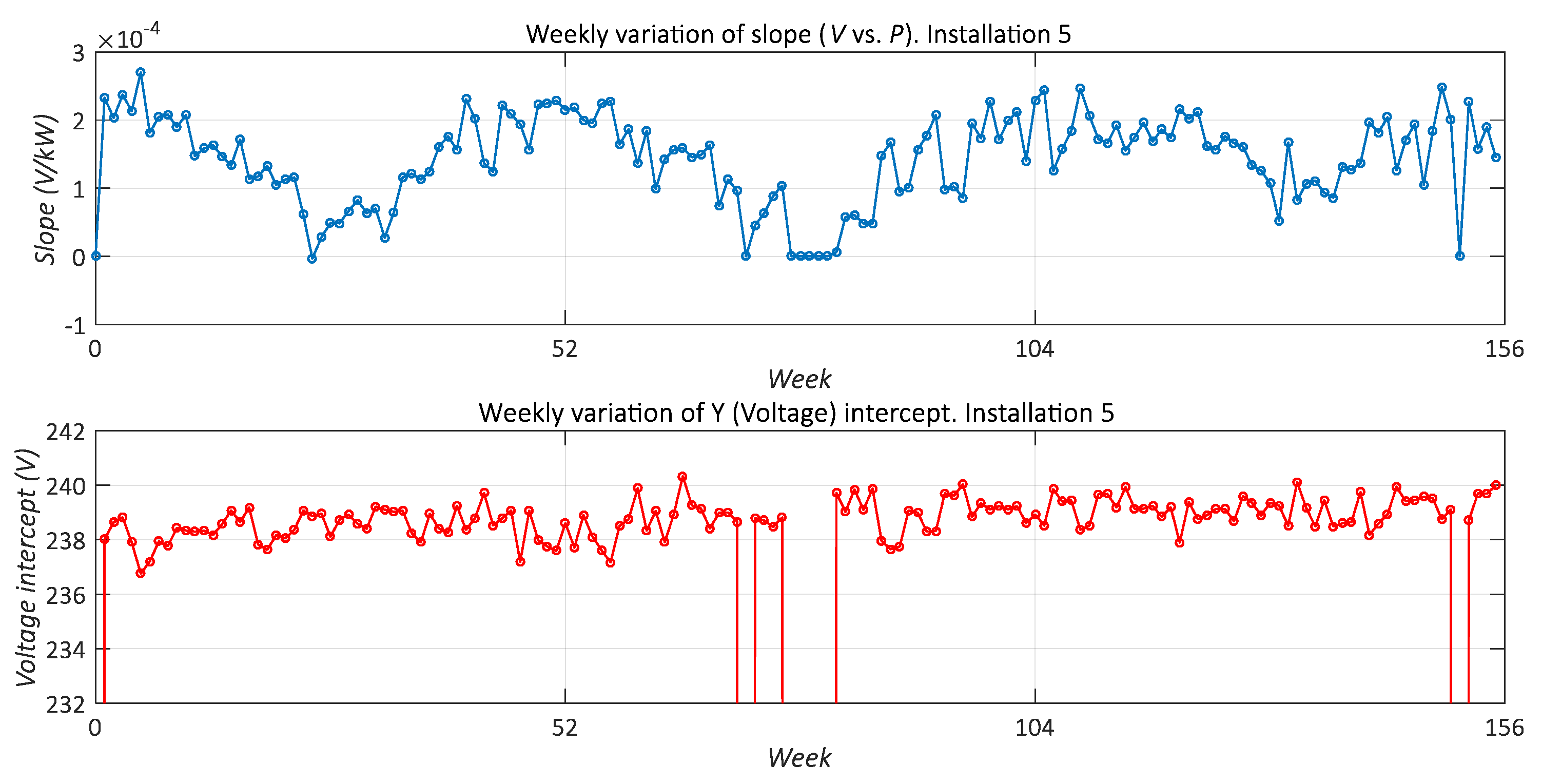
Figure 21 show the values found for the slope and Y-axis intercept of the VAC versus PAC ratios, calculated from the weekly data at each of the six PV plants studied. The values of the determination coefficients obtained in these weekly linear fits are shown in Figure 22. The periods in which there is no monitored data in the inverters were shown in these graphs as null values.
A summary of the maximum, minimum and average values of these parameters represented for each installation are shown in Table 2, Table 3 and Table 4.
In these Figure 16, Figure 17, Figure 18, Figure 19, Figure 20, Figure 21 and Figure 22, the first year corresponds to the first 52 weeks, the second year ends at week 104 and the third year ends at week 256, which are the weeks indicated on the X-axis of these figures.
The determination coefficients found, which have maximum values around 0.8 and lower average values (see Table 4), show that the grid voltage values have a certain dependence on the production of the plant injected into the grid, but that there are obviously more factors that are impacting in the values of this parameter, and that are external to the PV plants themselves. The variation of the value of this parameter over the monitored period also indicates that the impact of the production of PV installations on the grid voltage is not always constant, but also varies.
It can also be observed that the values of the Y-axis intercept found, which would correspond to the voltage values of the grid without PV power production, have a margin of variation throughout the period analysed. Table 3 shows the difference between the maximum and minimum values found in the regression lines. The largest range of variation of the grid voltage with no injection of PV production is found in the grid into which installation 2 injects, which in turn is the one in which the highest value of the slope was found. This shows that plant 2 is the one that is injecting into the least resilient network. In fact, as can be seen in Figure 17, over the three years of monitoring, the value of grid voltage without the PV plant’s production (value of the origin-axis intercept) increased by about 5 V, which shows that the state of the grid was modified independently of the operation of the PV installation. The most resilient grid would be those in which installation 6 injects (located in a residential area of a city), in which the voltage corresponding to the Y-axis intercept only varies by around 3 V during the entire period analysed, and the slope values found are among the lowest. The network in which installation 3 injects (located in a rural area) would also be among the most resilient, in which the slope is also one of those with the lowest values, together with lower values of the Y-axis intercept.
It can be seen in Figure 16, Figure 17, Figure 18, Figure 19, Figure 20 and Figure 21 that the slope values found vary from week to week. Except in the case of installation 2, where this behaviour is not observed, in the rest, it can be seen that during the summer months, the slope values are lower than those found during the winter months, indicating that the network is less resilient to PV production during the winter months. Although PV production is lower during the winter months, in summer, the maximum PV production coincides with the hours of highest temperature, and therefore, of highest electricity demand for air-conditioning, which in the geographical area analysed in this work represents a significant percentage of the electricity demand at those hours of the day [45], which could contribute to the fact that at those hours of highest production the voltage values increased less. Passey et al. [31] have already indicated that some impacts of distributed generation can be positive, for example, where PV generation is closely correlated to air-conditioning loads and hence reduces the peak network currents seen in the network.
It is obvious that the impact of the PV installation on the grid voltage value will depend on the one hand on the relative size and location of distribution generator (DG). But in addition, the specific pre-existing situation at each point in the network in terms of the connected loads nearby, their distribution topology and the methodology applied for voltage regulation are also influencing [43]. DG connected to the distribution network can significantly influence the aggregated impacts of all components in the grid [31]. If the grid impedance is higher, the PV output will have a greater effect and higher slope values will be obtained. If the voltage value prior to the injection of renewable production is low, the available margin for more renewable generation capacity is higher.
It was observed that with the parameters recorded by the inverters themselves, it is possible to assess how this impact is being, without the need to include additional measurement systems. With the values of slopes and 
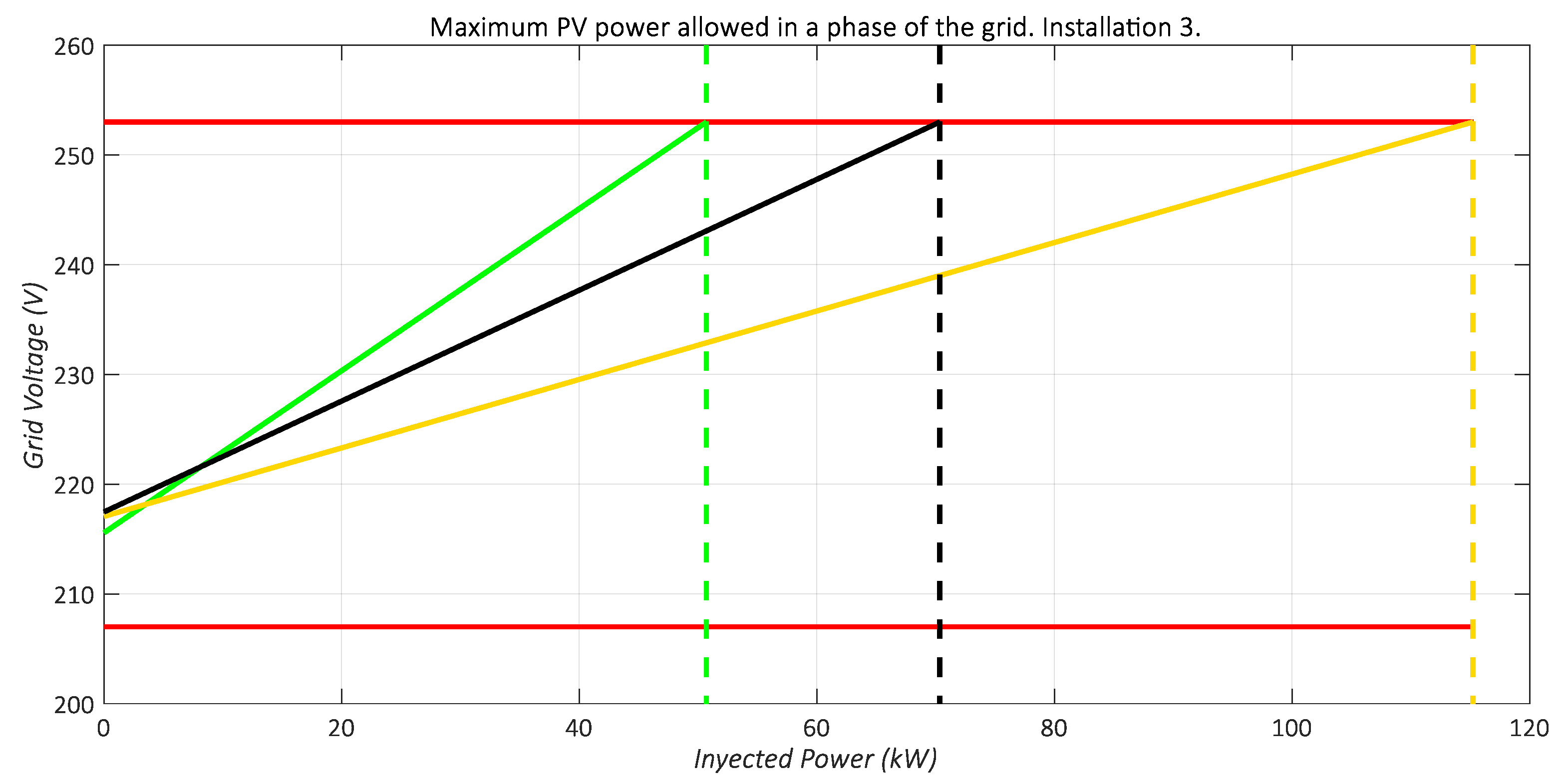
Y-axis intercepts found, it was also possible to estimate the maximum PV production capacity that each phase would admit in each of the grid points studied without exceeding the maximum values of the grid voltage indicated by the regulations, to avoid affecting consumers close to the PCCs with overvoltage values. This would make it possible to know the hosting capacity of the network in terms of the limit set by this parameter. For this purpose, the procedure for installation 3, shown as an example, is plot in Figure 23. In this Figure 23, the most unfavourable regression line is shown in green, the mean regression line in black and the most favourable line in yellow. In red are the maximum voltage values permitted by the standards. If the most unfavourable case is considered in this graph, the maximum PV power that could be injected in each phase at the same point would be around 50.7 kW. Above this power, the value of the grid voltage in the different phases could be higher than the maximum value of 253 V recommended by the regulations. Using the same procedure, an estimation of the hosting capacity was obtained in the rest of the PV installations, values that are shown in Table 5.
The results show that, as previously indicated, installations 3 and 6 were the most resilient with respect to PV production, and they would therefore admit a greater increase in the PV capacity that could be added per phase, in both cases more than 300% of the power already installed.
However, the most unfavourable slopes were considered for this calculation. Given that in some of the installations these maximum slope values had a small incidence and have only occurred during a few weeks in the three-year period, one could consider the option of further increasing the installed renewable capacity, considering lower slope values, and applying for example curtailment in the injection during these times of higher voltage increases.
Although the calculated hosting capacity has taken into account only the value of the nominal voltage at the PCC, the thermal limits of the network components should also be considered, although in LV networks and with the aim to limit voltage drops in conductors and by life-cycle cost aspects, usually larger conductors than those dictated by thermal limits are used [46]. Furthermore, to avoid reverse power flows to the transformer at the head of the line, the installed PV power should not exceed the maximum demand of the loads connected to the same distribution network during their peak production hours. The rating of an embedded generator connected below a particular transformer minus the minimum load in the same area must not exceed the maximum load in that area [46]. The analysis of these latter aspects is beyond the scope of this paper, as this information is not available to the authors, but, in any case, the most unfavourable result should be applied.
The results show that the values recorded by the inverters of the plants allow an assessment to be made of the impact that this type of installation is having on this grid parameter. Although the production of the PV plants leads to an increase in the grid voltage, it is not significantly affecting this parameter, which has already shown a variation in its value apart from the production of these renewable installations. However, obviously the hosting capacity of each network is limited, and it would have to be estimated for each grid parameter, in order not to give rise to future problems, or to plan the establishment of regulation mechanisms or control strategy to make this capacity even higher. The uses of the Battery Energy Storage System (BESS) to recharge during high power generation is a strategy that is proposed as a promising solution against the overvoltages limits [7,47,48,49]. More costly solutions in order to get an increment in grid capacity were also proposed as well, such as the use of Synchronous Condensers (SynCons) [50], the up gradation in distribution transformers to an increased power rating, replacing old conductors with new with higher capacity or reinforcement of LV feeders by additional parallel conductors [43]. Another option used to mitigate the voltage increase would be through the extraction of reactive power at the PCC, a strategy that is not yet exploited in LV network, which would require the development of more sophisticated and low cost power electronic interfaces in order to distributed generators can generate and control reactive power [46].

3.3. Imbalance of Network Voltage Values between Phases

This section analyses the imbalance or disequilibrium in voltage values among the three phases at each of the PCCs of the different PV installations analysed in this work, based on the grid voltage data recorded by the plants’ inverters. The voltage imbalance factor, that will depend on how the solar PVs and loads are distributed in different phases of the LV distribution network, have also been mentioned as one of the significant problems with high levels of PV penetration into LV distribution networks [8]. Imbalance can result in overheating and derating of induction motors, transformers and of small three-phase generators and can significantly affect the effectiveness of voltage regulation in the system [9].
To analyse the possible effect of the production of the PV plants on this imbalance, the disequilibrium, in absolute value, of the voltage in each of the phases (i), ∆Vgrid_phase_i versus the mean value of the voltages of the three phases Vgrid_phase_i, with i = 1, 2 and 3, was calculated by the Equation (1)
Δ V g r i d _ p h a s e _ i = | V g r i d _ p h a s e _ i ( i = 1 3 V g r i d _ p h a s e _ i 3 ) |
The result obtained have been represented in the form of colour maps. Some examples are shown below throughout the section.
Figure 24a shows the voltage imbalance in phase 2 measured by the inverters in PV installation 1. It can be seen in this case that the maximum imbalance between the voltages of this phase with respect to the average value of the three phases barely exceeds 4 V, but these higher values only occur very rarely. These maximum values of imbalance found are even lower than the variations in the voltage values that have been seen to exist in the phases themselves throughout the day. Analysing Figure 24b, which represents a histogram of the values represented in Figure 24a, it can be seen that the highest incidence of these imbalance corresponded to values lower than 1.5 V, but mostly those that predominate were the values very close to zero. In installation 1 to which this Figure 24 corresponds, the inverters are three-phase and, as previously indicated, they measure the voltage value in the grid 24 h a day. During the hours when the installation was not operating, it can be seen that the imbalance was around 1 V, and during production hours, when the inverters distribute the generated energy equally among the three phases, the imbalances were even lower, so that in this case, it can be observed that the operation of the three-phase generator may serve to reduce any existing phase voltage imbalance in the PCC [46]. In the rest of the inverters and phases of this installation, the results were within the same order of magnitude, and present the same behaviour. Gandhi et al. [9] indicate that the impact of PV to the system imbalance is sensitive to changes in the network configuration and to the existing imbalance of customers’ connection and consumption, and the voltage disequilibrium can be even reduced by increasing PV penetration. In the case of this installation, its high nominal power, and the balancing potential that the three-phase inverters can provide, could be contributing to this improvement in the balance between the three phases when there is production in the PV installation.
In Figure 25a, it is shown the imbalance of one of the phases, phase 3, determined from the data recorded by the two three-phase inverters of installation 2. The histogram of these values is shown in Figure 25b. It can be seen that the phase disequilibrium, which in this case was somewhat higher than that found in installation 1, was generally not directly related to the production of the PV plant, and the largest or smallest imbalance occurred at any time of the day. In the other two phases, as well as in the values recorded by the other inverter of this installation, the results were similar. The different profile of the histograms of the voltage imbalance values of installations 1 and 2 shows that the values of the imbalances do not depend on the operation of the plants but on the previous state of the grid itself, which will be conditioned by the loads that are connected to each of the three phases.
Figure 26a shows the voltage imbalance in phase 2 of installation 4, which has single-phase inverters. Initially, this figure shows that there are occasional voltage imbalances between the different phases, especially during the hours when the PV plant’s inverters start production and to a lesser extent during their disconnection at the end of the sunshine hours. However, these recorded imbalances are due to the fact that the inverters do not start operating, and therefore measuring, simultaneously on all three phases, but that the inverters connected to one of the phases may start operating a few minutes before those connected to the others.
During night-time hours, these inverters are in a disconnected state. They enter this state when the PV voltage is less than 60 V, and the production is too low to connect to the grid and even insufficient to feed the inverter itself. When the voltage coming from the PV field is between 60 and 220 V, the inverter goes into the initialisation state. The power supply from the PV array is sufficient to feed the inverter but there is not yet enough power to connect to the grid. The inverter will perform an automatic test of the electronic components of the equipment and switch to a state where it will monitor the network, taking measurements of the grid voltage, allowing it to verify that the requirements for connection to the grid are met. Therefore, during these initialisation minutes, these inverters are not yet injecting their production, but they are already measuring the grid voltage. Moreover, if the strings of the PV modules connected to each inverter are unevenly shaded, some inverters enter the initialisation state before others. Although in the end, they do inject simultaneously in all three phases, there are moments of time in which the inverters connected to one phase are already initialised and measuring the voltage values, and in other phases, they are still neither connected nor measuring, and therefore in the latter, the voltage value recorded is still zero. Therefore, at this time of day, there is an apparent voltage imbalance between the three phases, whose values are not real, but rather an apparent imbalance only because of some inverters starting to measure before others. This does not happen with three-phase inverters, which, as the same equipment injects into the three phases, the connection will be simultaneous and, in addition to distributing the production equally among the three phases, will generate measurements of the three phases simultaneously at any time of the day. It is also not possible to visualise the values of the grid voltage in the single-phase inverters analysed in this work during night-time hours, when the inverter does not operate and does not record these values.
If the data in Figure 26a are represented again but modifying the colour scale so that the imbalances of lesser magnitude can be better seen, the results shown in Figure 26b are obtained. In this case, it can be seen that the values of the voltage imbalances in phase 2 with respect to the average production of the three phases fluctuate throughout the day with a greater incidence in the early hours of the day and in the afternoon, in the winter months, when the days are shorter.
To see if this behaviour is related to the production of the plant, the imbalance, in absolute value, of the production in each of the phases (i), ∆PAC_grid_phase_i versus the average value of the production of the three phases PAC_grid_phase_i, with I = 1, 2 and 3, was determined in the same way as the imbalance of the voltage in the phases, by means of the Equation (2)
Δ P A C _ g r i d _ p h a s e _ i = | P A C _ g r i d _ p h a s e _ i ( i = 1 3 P A C _ g r i d _ p h a s e _ i 3 ) |
The results shown in Figure 27 were obtained in this way. It can be seen that during the first hours of the day, there was an imbalance in the grid voltage, but not in the production, so apparently this voltage imbalance was not caused by imbalances in the production of the PV plant between the phases. In the last hours of daily production, it is observed that there was an imbalance in both voltage and production values. With the data available, it is not possible to determine whether these voltage imbalances in the afternoon hours were a consequence of the production imbalances, or whether they were due to the same causes that deviated the voltage during the morning hours. It would be necessary to see if the state of the loads connected to the different phases changed throughout the day, which could make the network more sensitive to the presence of production imbalances between the three phases, but the authors did not have access to this information.
This is why, if a study of the voltage imbalance between phases needs to be carried out with data from the inverters, it is recommended to have inverter models that can record the voltage 24 h a day, in order to have more complete information on what happens in the grid throughout the day, and thus be able to have a greater amount of voltage values from the grid when there is no injection of production in the PV installation. As far as possible, three-phase inverters, which measure simultaneously in all three phases, should be available, or at least the PV modules of the different strings associated with inverters feeding into different phases should be located in such a way that they do not receive unequal shading in the early or late hours of the day, so that all inverters start operating simultaneously. Three-phase inverters also help to ensure that there is no imbalance in production between the three phases and can, depending on the size of the plant, help to reduce the imbalance between the phases at that point in the grid.
With respect to single-phase inverter measurements, it may also lead to errors in the interpretation of the phase-to-phase voltage imbalance data if there is a production failure in one or two of the inverters that are feeding into the different phases, and the rest of the inverters that have not failed to continue to produce electricity and record the grid voltage value. The failed inverters, not operating, will show zero voltage values, and therefore this apparent voltage imbalance between phases would be recorded for the whole period that the failure lasts, as it can be seen in Figure 28a for the case of installation 6. For example, on day 237 there is a fault in inverter 1, and therefore during the time that the fault lasts, the recording in this inverter of the grid voltage in phase 1, which is the phase in which it injects, is zero. As the rest of the inverters are working correctly and measure the grid voltage values in the other two phases, this apparent imbalance between the three phases appears. The same happens between days 581–585, 838–839 and 946–949 when there was also a failure in inverter 1, and therefore, this inverter stopped registering the grid voltage value. It is therefore important, when using inverter data to perform the analysis being carried out in this work, to know how the inverters are measuring, to be able to interpret the results correctly. If the inverter, when not working, does not measure the grid voltage, it is not feasible to assess the potential imbalance that could occur at such times of inverter failure. Therefore, it would be interesting for manufacturers to establish in the inverter configuration the option of continuing to measure the grid voltage in cases where the inverter fails and does not continue to inject current into the grid.
If the colour scale is again modified so that the smaller imbalance values can be better visualised, the results shown in Figure 28b are obtained. The main imbalances were observed in the first and last hours of production, because of the lack of synchronisation between the inverters at the switch-on and switch-off times. During the rest of the day, there are continuous fluctuations in the voltage values between the phases, but always of lesser magnitude. In this case, it can be verified that the imbalances of the voltage values do not have a direct relation to the imbalances in the output of the different phases, which is shown in Figure 29. In this plant, there is a string with shading, which in the early hours of the day, especially in the winter months, leads to an imbalance in the output of the three inverters. However, this does not have a direct consequence on the voltage imbalance values. Even without PV installations, there may already be imbalance due to unequal impedances and loads across the phases [9].
Despite these apparent imbalances, it has been verified that in this installation, 99% of the time periods in which there are measurement records during the three years analysed, the voltage imbalance measured in the three phases by the inverters was no greater than 1 V. It should be remembered that this installation is small, and also injects into one of the most resilient grids of those analysed in this study, which means that the voltage increase experienced with the increase in production was small, and that the voltage values of the three phases were not affected.

3.4. Analysis of the Grid Frequency Values Measured by the Inverters of PV Systems

One of the key parameters for grid stability is the value of the power signal frequency, which in general depends on the balance between generation and demand. Although the user can receive voltages in a range of variation around their nominal value without appreciable repercussions in most industrial or domestic applications, nevertheless, frequency variations are becoming increasingly important due to the growing number of clocks and automatisms connected to the electricity grid, for which not only the error at a given instant but also the error accumulated over time is important [46].
For frequency control, the mechanism traditionally used by conventional generators is inertial support, provided by large synchronous generators, mainly fossil-fuelled and hydroelectric generators [51]. However, one of the drawbacks of the presence of PV systems in the grid, given that they do not have mechanical elements, is that they cannot contribute to this control mechanism. If there is an increasing integration of PV systems that leads to decommitting of the traditional generators, then the amount inertia support will decrease. Moreover, since most PV systems are operating at Maximum Power Point Tracking (MPPT), they do not have any reserve for frequency regulation. This will result in an increase of the rate of change of frequency [9]. Initially, therefore, it is essential that the production of PV power does not contribute to at least an increase in the frequency variation of the grid. Since the inverters of the PV installations also measure the grid frequency, this parameter of the electrical signal and its possible variation with the production of the PV installations were also analysed.
With the data recorded by the inverters, it was found that, unlike the voltage, the frequency values recorded in the different phases by the inverters of the different installations did not show any dependence on the operation of the PV plant, and correct operation of the inverters was confirmed by monitoring the grid frequency in order to inject their production properly. An example is shown in Figure 30 for measurements recorded by an inverter of the PV installation 4 in one of the phases. In this figure, the values of 50 Hz ± 1% are shown in a red colour, which correspond to the range 49.5 and50.5 Hz, which are the limits set for this parameter for 99.5% of time by the standard UNE-EN 50160 [44]. The frequency value recorded by the inverters oscillated in a variation range that did not exceed ±0.1 Hz around 50 Hz, and these values did not seem to depend directly on the higher or lower production in the PV plants. For the rest of the installations, phases and during all the months of the period analysed, the behaviour found was very similar.
There was also no dependence between the values of the frequency variations with the variations of the PV power values, as can be seen in Figure 31. This figure shows that the greatest variations in frequency did not correspond to the greatest variations in the power generated by the PV installation. Although the production of the PV installation presents a variability that depends not only on the solar trajectory but also on the passing of clouds (a month has been chosen for this graph in which there are many days with passing clouds), this variability was not directly reflected in the variation of the frequency values measured by the inverter. The effect that PV production variability has on the grid will depend in each particular case on the variability of demand in that area as well as the presence of other possible sources of generation with other patterns of change in their production, considering the aggregate effect of all participants.
Figure 32 shows a colour map reflecting the value of the frequency over the entire monitoring period measured by the inverter connected to phase 1 in installation 4. It can be seen that the small oscillation of values of this parameter was not related to the production of the PV plants, which was shown in Figure 8. In the case of plants with three-phase inverters, the measurements of this parameter, as in the case of single-phase inverters, only take place during the hours when they are in operation, unlike the grid voltage, which was recorded by the three-phase inverters 24 h a day. Therefore, it is not possible to compare the value of the grid frequency during the hours of sunshine, with PV production, with those during the hours of the night, when the PV plants are not producing electricity. It would be interesting if inverters had the possibility to record this parameter throughout the day, to have more information on what happens to it when there is no production from the PV plant.
Still, though, the use of inverter measurements enables a first assessment to be made of the influence of the production of the PV installations and the variability of their production on the grid frequency values, without observing in this work that it is directly having a negative impact. Even if the presence of such non-synchronous generation power plants reduces the inertia of the system in terms of frequency control, at least the presence of production does not seem to contribute to changing this grid parameter. When these renewable installations are small, they have a negligible influence on the frequency. However, when a larger number of such installations are connected, their aggregate impact could be significant. In the future, with the increasing penetration of such installations in the grid, it will also be necessary for these installations to be able to participate in the frequency regulation of the grid, which would require, e.g., not working at full capacity, in order to have a reserve for continuous or occasional frequency control [28]. In addition, inverters with power electronics that can respond to increases or variations in power flows would be required, and this response could take place more quickly than is currently the case with conventional generators, which could even be an advantage [46,52].

4. Conclusions

In this work, an analysis of some power quality parameters was carried out based on the data recorded over a three-year period by the inverters of six small PV installations, distributed in a province in the south of Spain, and which inject their production at different points of various LV distribution networks. The possible impact of the production of these renewable installations on the voltage and frequency values of the grid was analysed.
With the data measured by the inverters, it was found that, as production increased at the various plants, there was an increase in the grid voltage. This increase was coupled with the previous voltage variation in the grid itself, which is independent of the energy production in these plants. However, the slopes found corresponding to the relationship between the voltage and the production of the PV plants were of small value, and at no time did they lead to the voltage of the grid exceeding the limits recommended by the current regulations. Therefore, although the PV installations were impacting on each of the LV distribution networks in which they were injecting their production, there are other factors that were contributing to power quality issues in those networks, to the same or greater extent than the PV installations.
The values found for both the slopes and the voltage in the grid without injection of the plants’ production depended not only on the size of the PV installation, but also on the state and the strength of the grid itself. Even these values did not remain constant over the three years. For example, there was one installation in which the grid voltage without PV production was increasing over the three years of the monitored period, regardless of the operation of the plant itself. Others showed a certain periodicity throughout the year in the value of the slopes.
The value of the slopes found also allowed us to estimate the hosting capacity for this type of installation that these LV networks would have, to avoid the effect of PV production leading to voltage values that are not recommended by the regulations.
Regarding the imbalance of the voltage values in the three phases, also analysed in the work, different results were obtained depending on the plant studied. It was not found that the production of the plants directly causes an additional imbalance to the one already present in the grid due to the distribution of loads between the three phases. It was even observed that if three-phase inverters are available, there can be an improvement in this imbalance when they are injecting their production. However, the way in which inverters record voltage data can lead to errors in the interpretation of this imbalance, which makes it necessary to know the different operating states of the inverters and how they record the grid voltage in each of them, recommending that the grid voltage is a parameter that is measured in any operating state of the inverters. The best option in this respect would be the use of three-phase inverters, which inject in a balanced way in all three phases. In the case of using single-phase inverters, it is important to balance the PV production on all three phases well, and to avoid unequal shading between the panels producing in the inverters connected to the different phases.
The influence of the output of PV plants on the grid frequency values measured by inverters was also analysed in this work. However, no variation of the frequency values was found to be related to the generation of electricity in these installations. For this analysis, a faster sampling period than the one used by inverters would be advisable. It would also be recommended for inverters to be able to measure this parameter 24 h a day.
It is obvious that further integration of renewable generation facilities into LV distribution grids would have to be accompanied by improvements in the state of the network analysis and grid control, which would require improvements in metering and data acquisition, communications, and information processing systems. Furthermore, the impact of each plant will depend in each case not only on its size and characteristics, but also on the strength of the network and the state of the grid in each specific PCC, so it is essential to perform this analysis for all renewable generation installations that are connected to the grid. Therefore, PV installation monitoring systems themselves can make an important contribution in this respect, to be able to make an initial assessment of the impact of each PV installation on some of the grid parameters without the need for additional measurement systems.
Knowing how these inverters measure, and in each case having inverter models that can record grid parameters throughout the day, not only during the time when they produce energy, to assess the state of the grid without production injection, is essential to be able to use this resource available to most small PV installations.
In future work, the intention is to carry out this analysis in some PV installations with higher rated power, in the order of MW, and even installations that feed into medium voltage (MV) grids, with the aim to analyse the impact on the grid of the production of these larger plants. Although the inverter data have an acceptable accuracy, it would also be interesting to measure simultaneously with the inverters and with a network analyser to calibrate the inverter measurements, study to be carried out by the authors in the future. This equipment was not available for this work. However, the data used in this paper do allow us to see the relative variation between the voltage values with and without PV production, or the variation of results from one installation to another, which shows that the values found and the possible increase in voltage depended not only on the installation characteristics, but also on the specific state of network in each PCC.

Author Contributions

I.S. proposed the topic of study for the paper, carried out the literature review and proposed the methodology. She participated in the data processing, and in the writing and editing the manuscript. She carried out the supervision of the work for the implementation of the paper. J.G.-Q. carried out the analysis and graphical representation of some data, and he also participated in the writing of the paper. G.M.-A. also carried out the analysis and graphical representation of some data, and he also participated in the writing of the paper. D.T.-M. participated in the preparation of the data, from the inverter monitoring files, to convert them into matrices in order to facilitate their use for the analysis of the work. He also participated in the writing of the paper. R.J.R.-C. participated in carrying out the literature review and in writing and editing the paper. He participated in the funding acquisition. M.G.-R. participated in the data processing and in the writing and editing of the paper. All authors have read and agreed to the published version of the manuscript.

Funding

This research was supported by the Project Monitoring and Integration of energy data with Seamless Temporal Accuracy for photovoltaic plants (MISTA), PID2019-108953RA-C22, funded by the Spanish Ministry of Economy and Competitiveness.

Institutional Review Board Statement

Not applicable.

Informed Consent Statement

Not applicable.

Acknowledgments

The authors would like to thank the company Solar del Valle SL, which, via their collaboration agreements with our Research Group, provided data monitored in photovoltaic installations.

Conflicts of Interest

The authors declare no conflict of interest.

References

  1. IRENA (International Renewable Energy Agnecy). Renewable Energy Statistics. 2020. Available online: https://www.irena.org/publications/2020/Jul/Renewable-energy-statistics-2020 (accessed on 26 July 2021).
  2. European Commission. A European Green Deal. Available online: https://ec.europa.eu/info/strategy/priorities-2019-2024/european-green-deal_en (accessed on 26 July 2021).
  3. Schmela, M. Global Market Outlook for Solar Power 2019–2032. 2019. Available online: https://www.solarpowereurope.org/wp-content/uploads/2019/07/SolarPower-Europe_Global-Market-Outlook-2019-2023.pdf (accessed on 27 July 2021).
  4. Schmela, M. Global market outlook for solar power 2018–2022. 2018. Available online: https://www.solarpowereurope.org/wp-content/uploads/2018/09/Global-Market-Outlook-2018-2022.pdf (accessed on 27 July 2021).
  5. PVinsights. Solar PV Module Weekly Spot Price. 2020. Available online: http://pvinsights.com/ (accessed on 28 July 2021).
  6. IEA Renewables 2019. Market Analysis and Forecasts to 2024. 2019. Available online: https://www.iea.org/reports/renewables-2019 (accessed on 30 July 2021).
  7. Aleem, S.A.; Hussain, S.M.S.; Ustun, T.S. A Review of Strategies to Increase PV Penetration Level in Smart Grids. Energies 2020, 13, 636. [Google Scholar] [CrossRef] [Green Version]
  8. Haque, M.M.; Wolfs, P. A review of high PV penetrations in LV distribution networks: Present status, impacts and mitigation measures. Renew. Sustain. Energy Rev. 2016, 62, 1195–1208. [Google Scholar] [CrossRef]
  9. Gandhi, O.; Kumar, D.S.; Rodríguez-Gallegos, C.D.; Srinivasan, D. Review of power system impacts at high PV penetration Part I: Factors limiting PV penetration. Sol. Energy 2020, 210, 181–201. [Google Scholar] [CrossRef]
  10. Panchenko, V.A. Solar Roof Panels for Electric and Thermal Generation. Appl. Sol. Energy 2018, 54, 350–353. [Google Scholar] [CrossRef]
  11. Protopapadaki, C. A Probabilistic Framework towards Metamodeling the Impact of Residential Heat Pumps and PV on Low-Voltage Grids; Faculty of Engineering Science, KU Leuven: Leuven, Belgium, 2018. [Google Scholar]
  12. Karimi, M.; Mokhlis, H.; Naidu, K.; Uddin, S.; Bakar, A.H.A. Photovoltaic penetration issues and impacts in distribution network—A review. Renew. Sustain. Energy Rev. 2016, 53, 594–605. [Google Scholar] [CrossRef]
  13. Shivashankar, S.; Mekhilef, S.; Mokhlis, H.; Karimi, M. Mitigating methods of power fluctuation of photovoltaic (PV) sources—A review. Renew. Sustain. Energy Rev. 2016, 59, 1170–1184. [Google Scholar] [CrossRef]
  14. Ravindran, V.; Busatto, T.; Ronnberg, S.K.; Meyer, J.; Bollen, M. Time-varying interharmonics in different types of grid-tied PV inverter systems. IEEE Trans. Power Deliv. 2019, 35, 483–496. [Google Scholar] [CrossRef]
  15. Kuznetsov, P.; Yuferev, L.; Voronin, D.; Panchenko, V.A.; Jasiński, M.; Najafi, A.; Leonowicz, Z.; Bolshev, V.; Martirano, L. Methods Improving Energy Efficiency of Photovoltaic Systems Operating under Partial Shading. Appl. Sci. 2021, 11, 10696. [Google Scholar] [CrossRef]
  16. Santiago, I.; Esquivel-Martin, J.L.; Trillo-Montero, D.; Real-Calvo, R.J.; Pallarés-López, V. Classification of Daily Irradiance Profiles and the Behaviour of Photovoltaic Plant Elements: The Effects of Cloud Enhancement. Appl. Sci. 2021, 11, 5230. [Google Scholar] [CrossRef]
  17. Tomson, T. Transient processes of solar radiation. Theor. Appl. Climatol. 2013, 112, 403–408. [Google Scholar] [CrossRef]
  18. Lappalainen, K.; Valkealahti, S. Recognition and modelling of irradiance transitions caused by moving clouds. Sol. Energy 2015, 112, 55–67. [Google Scholar] [CrossRef]
  19. Espinosa-Gavira, M.J.; Agüera-Pérez, A.; Palomares-Salas, J.-C.; González-de-la-Rosa, J.-J.; Sierra-Fernández, J.-M.; Florencias-Oliveros, O. Cloud motion estimation from small-scale irradiance sensor networks: General analysis and proposal of a new method. Sol. Energy 2020, 202, 276–293. [Google Scholar] [CrossRef]
  20. Santiago, I.; López-Rodríguez, M.A.; Gil-de-Castro, A.; Moreno-Munoz, A.; Luna-Rodríguez, J.J. Energy consumption of audiovisual devices in the residential sector: Economic impact of harmonic losses. Energy 2013, 60, 292–301. [Google Scholar] [CrossRef]
  21. Ahmed, N.; Sedky, A.; Fatehy, A.; Foda, M. Impact of grid-connected photovoltaic system on power-quality indices and its output variations with temperature. CIRED Open Access Proc. J. 2017, 2017, 710–714. [Google Scholar] [CrossRef] [Green Version]
  22. Ebad, M.; Grady, W.M. An approach for assessing high-penetration PV impact on distribution feeders. Electr. Power Syst. Res. 2016, 133, 347–354. [Google Scholar] [CrossRef]
  23. Ali, M.H.; Rabhi, A.; Hajjaji, A.E.; Tina, G.M. Real Time Fault Detection in Photovoltaic Systems. Energy Procedia 2017, 111, 914–923. [Google Scholar] [CrossRef]
  24. Farhoodnea, M.; Mohamed, A.; Shareef, H.; Zayandehroodi, H. Power quality impact of grid-connected photovoltaic generation system in distribution networks. In Proceedings of the SCOReD 2012—2012 IEEE Student Conference on Research and Development, Pulau Pinang, Malaysia, 5–6 December 2012. [Google Scholar]
  25. Zhu, Y.; Hao, J.; Li, X.; Tang, Q.; Xia, R. Research on harmonic and overvoltage of photovoltaic power plant electricity energy collection system based on passive network model. J. Eng. 2017, 2017, 789–794. [Google Scholar] [CrossRef]
  26. Mahmud, N.; Zahedi, A. Review of control strategies for voltage regulation of the smart distribution network with high penetration of renewable distributed generation. Renew. Sustain. Energy Rev. 2016, 64, 582–595. [Google Scholar] [CrossRef]
  27. Chidurala, A. High Penetration of PV Systems in Low Voltage Distribution Networks: Investigation of Power Quality Challenges and Mitigation. Ph.D. Thesis, School of Information Technology and Electrical Engineering, The University of Queensland, Brisbane, Australia, 2016. [Google Scholar] [CrossRef] [Green Version]
  28. Shah, R.; Mithulananthan, N.; Bansal, R.C.; Ramachandaramurthy, V.K. A review of key power system stability challenges for large-scale PV integration. Renew. Sustain. Energy Rev. 2015, 41, 1423–1436. [Google Scholar] [CrossRef]
  29. Kumar, D.S.; Gandhi, O.; Rodríguez-Gallegos, C.D.; Srinivasan, D. Review of power system impacts at high PV penetration Part II: Potential solutions and the way forward. Sol. Energy 2020, 210, 202–221. [Google Scholar] [CrossRef]
  30. Kenneth, A.P.; Folly, K. Voltage rise issue with high penetration of grid connected PV. In IFAC Proceedings Volumes (IFAC-PapersOnline); Elsevier: Amsterdam, The Netherlands, 2014. [Google Scholar]
  31. Passey, R.; Spooner, T.; MacGill, I.; Watt, M.; Syngellakis, K. The potential impacts of grid-connected distributed generation and how to address them: A review of technical and non-technical factors. Energy Policy 2011, 39, 6280–6290. [Google Scholar] [CrossRef]
  32. Ravindran, V.; Ronnberg, S.K.; Busatto, T.; Bollen, M.H.J. Inspection of interharmonic emissions from a grid-tied PV inverter in North Sweden. In Proceedings of the International Conference on Harmonics and Quality of Power, ICHQP, Ljubljana, Slovenia, 13–16 May 2018. [Google Scholar]
  33. Rönnberg, S.; Gutiérrez-Ballesteros, E.; Gil-de-Castro, A.; Westman, M.; Brodin, M. Long-term power quality measurements in medium voltage networks. In Proceedings of the 25th International Conference on Electricity Distribution (CIRED), Madrid, Spain, 3–6 June 2019; Paper No. 652. pp. 1–5. [Google Scholar]
  34. De Souza, V.R.F.B.; Filho, M.A.; De Oliveira, K.C. Analysis of power quality for photovoltaic systems connected to the grid. In Proceedings of the International Conference on Harmonics and Quality of Power, ICHQP, Belo Horizonte, Brazil, 16–19 October 2016. [Google Scholar]
  35. Fekete, K.; Klaic, Z.; Majdandzic, L. Expansion of the residential photovoltaic systems and its harmonic impact on the distribution grid. Renew. Energy 2012, 43, 140–148. [Google Scholar] [CrossRef]
  36. Rönnberg, S.; Bollen, M.; Larsson, A. Grid impact from PV-installations in northern Scandinavia. In Proceedings of the 22nd International Conference and Exhibition on Electricity Distribution (CIRED 2013), Stockholm, Sweden, 10–13 June 2013; IET Conference Publications: Stevenage, UK, 2013. [Google Scholar]
  37. Tumbelaka, H.H.; Muljadi, E.; Gao, W. Power quality improvement utilizing photovoltaic generation connected to a weak grid. In Proceedings of the 2017 IEEE Energy Conversion Congress and Exposition, ECCE 2017, Cincinnati, OH, USA, 1–5 October 2017. [Google Scholar]
  38. Cardona, A.J.A.; Chica, C.A.P. Power quality analysis of a 6 kW photovoltaic system interconnected with the distribution grid of a laboratories building. In Proceedings of the 2017 3rd IEEE Workshop on Power Electronics and Power Quality Applications, PEPQA 2017—Proceedings, Bogota, Colombia, 31 May–2 June 2017. [Google Scholar]
  39. Miller, W.; Liu, A.; Amin, Z.; Wagner, A. Power Quality and Rooftop-Photovoltaic Households: An Examination of Measured Data at Point of Customer Connection. Sustainability 2018, 10, 1224. [Google Scholar] [CrossRef] [Green Version]
  40. SMA. Available online: https://www.sma-america.com/service-support/downloads.html (accessed on 30 November 2021).
  41. Trillo-Montero, D.; Santiago, I.; Luna-Rodriguez, J.J.; Real-Calvo, R. Development of a software application to evaluate the performance and energy losses of grid-connected photovoltaic systems. Energy Convers. Manag. 2014, 81, 144–159. [Google Scholar] [CrossRef]
  42. Santiago, I.; Trillo Montero, D.; Luna Rodríguez, J.J.; Moreno Garcia, I.M.; Palacios Garcia, E.J. Graphical diagnosis of performances in photovoltaic systems: A case study in southern Spain. Energies 2017, 10, 1964. [Google Scholar] [CrossRef] [Green Version]
  43. Chaudhary, P.; Rizwan, M. Voltage regulation mitigation techniques in distribution system with high PV penetration: A review. Renew. Sustain. Energy Rev. 2018, 82, 3279–3287. [Google Scholar] [CrossRef]
  44. European Standard EN 50160: 2011; Voltage Characteristics of Electricity Supplied by Public Electricity Networks. European Committee for Electrotechnical Standardization (CENELEC): Brussels, Belgium, 2011.
  45. Palacios-Garcia, E.J.; Moreno-Munoz, A.; Santiago, I.; Flores-Arias, J.M.; Bellido-Outeirino, F.J.; Moreno-Garcia, I.M. A stochastic modelling and simulation approach to heating and cooling electricity consumption in the residential sector. Energy 2018, 44, 1080–1091. [Google Scholar] [CrossRef]
  46. Freiris, L.; Infield, D. Renewable Energy in Power Systems; Willey, Ed.; John Willey and Sons, Ltd.: Chichester, UK, 2008. [Google Scholar]
  47. Etherden, N.; Bollen, M.H.J. Increasing the hosting capacity of distribution networks by curtailment of renewable energy resources. In Proceedings of the 2011 IEEE PES Trondheim PowerTech: The Power of Technology for a Sustainable Society, Powertech 2011, Trondheim, Norway, 19–23 June 2011. [Google Scholar]
  48. Etherden, N.; Bollen, M.H.J.; Ackeby, S.; Lennerhag, O. the Transparant Hosting-Capacity Approach—Overview, Applications and Developments. In Proceedings of the 23rd International Conference and Exhibition on Electricity Distribution, Lyon, France, 15–18 June 2015. [Google Scholar]
  49. Etherden, N. Increasing the Hosting Capacity of Distributed Energy Resources Using Storage and Communication. Ph.D. Thesis, Lulea University of Technology, Luleå, Sweden, 2012. [Google Scholar]
  50. Hadavi, S.; Mansour, M.Z.; Bahrani, B. Optimal Allocation and Sizing of Synchronous Condensers in Weak Grids with Increased Penetration of Wind and Solar Farms. IEEE J. Emerg. Sel. Top. Circuits Syst. 2021, 11, 199–209. [Google Scholar] [CrossRef]
  51. Denholm, P.; Sun, Y.; Mai, T. An Introduction to Grid Services: Concepts, Technical Requirements, and Provision from Wind; Technical Report NREL/TP-6A20-72578; National Renewable Energy Laboratory (NREL): Golden, CO, USA, 2019; pp. 1–52.
  52. Kroposki, B.; Johnson, B.; Zhang, Y.; Gevorgian, V.; Denholm, P.; Hodge, B.-M.; Hannegan, B. Achieving a 100% Renewable Grid: Operating Electric Power Systems with Extremely High Levels of Variable Renewable Energy. IEEE Power Energy Mag. 2017, 15, 61–73. [Google Scholar] [CrossRef]
Figure 1. Geographical distribution of the six PV plants analysed in the province of Córdoba, South Spain. The numbers correspond to the order of the installations shown in Table 1.
Applsci 12 01138 g001
Figure 2. Values of the current generated in one of the inverters in PV plant 1 and values of the grid voltage measured by the inverter in one of the phases.
Applsci 12 01138 g002
Figure 3. Values of the grid voltage measured by an inverter in one of the phases without and with electricity production in the PV plant 1.
Applsci 12 01138 g003
Figure 4. Values of the current generated in one of the inverters in PV plant 2 and values of the grid voltage measured by the inverter in one of the phases.
Applsci 12 01138 g004
Figure 5. Values of the grid voltage measured by an inverter in one of the phases without and with electricity production in the PV plant 2.
Applsci 12 01138 g005
Figure 6. Values of the current generated in one of the inverters in PV plant 3 and values of the grid voltage measured by one of the inverters in one of the phases.
Applsci 12 01138 g006
Figure 7. Values of the grid voltage measured by an inverter in one of the phases without and with electricity production in the PV plant 3.
Applsci 12 01138 g007
Figure 8. Values of the current generated in one of the inverters in PV plant 4 and values of the grid voltage measured by one of the inverters in one of the phases.
Applsci 12 01138 g008
Figure 9. Values of the grid voltage measured by an inverter in one of the phases without and with electricity production in the PV plant 4.
Applsci 12 01138 g009
Figure 10. Values of the current generated in one of the inverters in PV plant 5 and values of the grid voltage measured by one of the inverters in one of the phases.
Applsci 12 01138 g010
Figure 11. Values of the grid voltage measured by an inverter in one of the phases without and with electricity production in the PV system 5.
Applsci 12 01138 g011
Figure 12. Values of the current generated in one of the inverters in PV plant 6 and values of the grid voltage measured by one of the inverters in one of the phases.
Applsci 12 01138 g012
Figure 13. Values of the grid voltage measured by an inverter in one of the phases without and with electricity production in the PV plant 6.
Applsci 12 01138 g013
Figure 14. Values of the grid voltage measured by the inverters in one of the phases in each of the PV installations analysed, when there is production from the installation being fed into the grid.
Applsci 12 01138 g014
Figure 15. Ratio between the values of the grid voltage VAC on one of the phases versus the values of the PAC power produced in PV installations (a) Installation 1 measured during month 5 (May), (b) Installation 2 measured during month 11 (November), (c) Installation 3 measured during month 9 (September), (d) Installation 4 measured during month 3 (March), (e) Installation 5 measured during month 4 (April) and (f) Installation 6 measured during month 10 (October).
Applsci 12 01138 g015aApplsci 12 01138 g015b
Figure 16. Weekly variation of the slope and the ordinate at the origin corresponding to the VAC versus PAC regressions in PV installation 1 during the three years monitored.
Applsci 12 01138 g016
Figure 17. Weekly variation of the slope and ordinate at the origin corresponding to the VAC versus PAC regressions in PV installation 2 during the three years monitored.
Applsci 12 01138 g017
Figure 18. Weekly variation of the slope and the ordinate at the origin corresponding to the VAC versus PAC regressions in PV installation 3 during the three years monitored.
Applsci 12 01138 g018
Figure 19. Weekly variation of the slope and the ordinate at the origin corresponding to the VAC versus PAC regressions in PV installation 4 during the three years monitored.
Applsci 12 01138 g019
Figure 20. Weekly variation of the slope and the ordinate at the origin corresponding to the VAC versus PAC regressions in PV installation 5 during the three years monitored.
Applsci 12 01138 g020
Figure 21. Weekly variation of the slope and the ordinate at the origin corresponding to the VAC versus PAC regressions in PV installation 6 during the three years monitored.
Applsci 12 01138 g021
Figure 22. Weekly variation of the determination coefficient corresponding to the VAC versus PAC regressions in the PV installations during the three years monitored. (a) Results for Installation 1, (b) Results for Installation 2, (c) Results for Installation 3, (d) Results for Installation 4, (e) Results for Installation 5 and (f) Results for Installation 6.
Applsci 12 01138 g022
Figure 23. Maximum values of PV power that would be admitted in each phase in the network at the PCC of installation 3, depending on the maximum (green line), average (black line) and minimum (yellow line) slopes and Y-axis intercept.
Applsci 12 01138 g023
Figure 24. Grid voltage imbalance on phase 2, measured by inverter 2 in PV installation 1 (a) and the histogram of these grid voltage imbalance values (b).
Applsci 12 01138 g024
Figure 25. Grid voltage imbalance on phase 3, measured by inverter 1 in PV installation 2 (a) and the histogram of these grid voltage imbalance values (b).
Applsci 12 01138 g025
Figure 26. Grid voltage imbalance on phase 2, measured by inverter 2 in PV installation 4 (a) and these grid voltage imbalance values detailing smaller deviations (b).
Applsci 12 01138 g026
Figure 27. PV production imbalance on phase 2 with respect to the production on the three phases, measured by inverter 2 in PV installation 4.
Applsci 12 01138 g027
Figure 28. Grid voltage imbalance on phase 1, measured by inverter 1 in PV installation 6 (a) and these grid voltage imbalance values detailing smaller deviations (b).
Applsci 12 01138 g028
Figure 29. PV production imbalance on phase 1 respect the production on the three phases, measured by inverter 1 in PV installation 6.
Applsci 12 01138 g029
Figure 30. Relationship between the values of the grid frequency in one of the phases versus the values of the power produced PAC in the PV 4 system measured during month 11 (November).
Applsci 12 01138 g030
Figure 31. Relationship between the variations of the grid frequency in one of the phases versus the values of the variations of the PAC power produced in the PV 4 installation measured during month 11 (November).
Applsci 12 01138 g031
Figure 32. Relationship between the values of the grid frequency in one of the phases versus the values of the PAC power produced in the PV 4 installation measured during month 11 (November).
Applsci 12 01138 g032
Table 1. Main technical characteristics of PV plants analysed.
Plant 1Plant 2Plant 3Plant 4Plant 5Plant 6
Total power (kW)672.0217.636.722.2100.217.8
Number of inverters 3263183
Inverter modelSMA SC-200SMA SC-100SMA SMC-5000SMA SMC-7000HVSMA SMC-5000ASMA SMC-5000
Number of modules per inverter128064036382636
Total number of modules38401280216114468108
Module modelSuntech, STP 175S-24/AcBP-3170Suntech, STP 170S-24/AcBosch, c-Si M48195Atersa, A-214PBP-3165
Module nominal power (W)175170170195214165
Single-phase or Three-phaseThree-phaseThree-phaseSingle-phaseSingle-phaseSingle-phaseSingle-phase
Rooftop or groundRooftop and groundRooftopRooftopRooftopRooftopRooftop
Geographical locationCarcabueyPozoblancoCarcabueyHinojosa del DuqueCórdobaCórdoba
Rural or city areaRural,
industrial area
Rural,
industrial area
Rural,
industrial area
Rural,
industrial area
City,
industrial area
City,
residential area
Latitude37.46388938.3593937.44638938.48181237.89916737.896389
Longitude−4.268611−4.84436−4.271944−5.123581−4.715278−4.795556
Table 2. Maximum, minimum, and average values of the slope obtained by correlating weekly over the three-year period the values of the grid voltage versus the power generated in the PV installations.
Max SlopeMin SlopeAverage Slope
PV Installation 10.0550.0210.039
PV Installation 20.130.0500.078
PV Installation 30.000740.000310.00050
PV Installation 40.950.0510.5
PV Installation 50.00027−0.00000310.00015
PV Installation 60.00074−0.000300.00027
Table 3. Maximum, minimum, and average values of the Y-axis-intercept obtained by correlating weekly over the three-year period the values of the grid voltage versus the power generated in the PV installations.
Max VAC InterceptMin VAC InterceptAverage VAC InterceptDifference between Max and Min
PV Installation 1236.83232.15234.894.68
PV Installation 2243.56233.40237.8910.16
PV Installation 3219.78215.23217.474.55
PV Installation 4237.83232.33236.035.50
PV Installation 5240.33236.76238.803.57
PV Installation 6236.81233.54232.893.27
Table 4. Maximum, minimum, and average values of the determination coefficient R2 obtained by correlating weekly over the three-year period the values of the grid voltage versus the power generated in the PV installations.
Max Determination CoefficientMin Determination CoefficientAverage Determination Coefficient
PV Installation 10.890.350.73
PV Installation 20.840.510.72
PV Installation 30.880.310.70
PV Installation 40.740.040.44
PV Installation 50.79−0.010.51
PV Installation 60.63−0.260.28
Table 5. PV power values allowed in each phase at the grid feed-in point of each PV installation, obtained from the maximum values of slope and Y-axis intercept obtained in the weekly regressions.
Current Nominal Power of the Plant (kW)Current Nominal Power Per Phase (kW)Maximum Nominal Power Per Phase with the Most Unfavourable Slope (kW)Increase Allowed (kW)Increase in Power Compared to the Current Installed Power Per Phase (%)
PV Installation 1672.0224.0364.7140.762.8
PV Installation 2217.672.5142.069.595.8
PV Installation 336.712.250.738.5314.2
PV Installation 422.27.418.210.8145.7
PV Installation 5100.233.460.026.679.7
PV Installation 617.85.925.519.6329.3
Publisher’s Note: MDPI stays neutral with regard to jurisdictional claims in published maps and institutional affiliations.

