Bearing Fault Diagnosis of Split Attention Network Based on Deep Subdomain Adaptation

Abstract

The insufficient learning ability of traditional convolutional neural network for key fault features, as well as the characteristic distribution of vibration data of rolling bearing collected under variable working conditions is inconsistent, and decreases the bearing fault diagnosis accuracy. To address the problem, a deep subdomain adaptation split attention network (SPDSAN) is proposed for intelligent fault diagnosis of bearings. Firstly, the time-frequency diagram of a vibration signal is obtained by the continuous wavelet transform to show the time-frequency characteristics. Secondly, a residual split-attention network (ResNeSt) that integrates multi-path and channel attention mechanisms is constructed to extract the key features of rolling bearings to prevent feature loss. Then, a subdomain adaptation layer is added to ResNeSt to align the distribution of related subdomain data by minimizing the local maximum mean difference. Finally, the SPDSAN model is validated using the Case Western Reserve University datasets. The results show that the average diagnostic accuracy of the proposed method is 99.9% when the test set samples are not labeled, which is higher compared to the accuracy of other mainstream intelligent fault diagnosis models.

1. Introduction

Rotating machinery is widely used in aerospace, automobile manufacturing, wind power generation and other important engineering fields. Rolling bearing is a key component in rotating machinery. Because this mechanical equipment often operates under complex working conditions, bearings are prone to pitting, breaking, gluing and other failures, which will lead to the paralysis of the mechanical equipment and cause significant economic losses [1]. Statistical analysis results provided by multiple studies have shown that more than 40% of the equipment faults are related to bearings [2]. Thus, how to improve the fault diagnosis of bearings under variable working conditions is related to the stable operation of the whole equipment and production line.

The traditional fault diagnosis method determines the equipment health state by establishing the corresponding dynamic model. For instance, Ambrokiewicz et al. [3] not only considered the bearing internal stiffness, damping, clearance and other nonlinear characteristics, but also took the bearing external load, eccentricity and other characteristics as factors affecting the normal operation of the bearing ball. The dynamics model of the ball bearing motion process with two degrees of freedom was established to reveal the dimensionless relationship and the influence on the system response. In the study by Huangfu et al. [4], the traditional loaded tooth contact analysis (LTCA) method was extended to calculate the mesh stiffness and contact stress of spalled gear pairs, and established a novel dynamic model for spalled gear pairs to describe the dynamic response of the gear pair under different spall modes. Such methods heavily rely on the researcher expertise, and specific devices are needed to establish specific dynamic models, greatly limiting their applicability [5].

In addition, some scholars analyze the characteristic frequency of faults. For instance, Arkadiusz et al. [6] used Fourier transform and recurrence analysis to analyze the vibration signal during engine operation, and could accurately determine the location of the failed cylinder. In order to solve the problem that composite bearing faults are difficult to diagnose, Wang et al. [7] first established a functional model of bearing vibration signals, and then a single fault frequency feature set was separated through decoupling, so as to complete the diagnosis of composite faults. Almounajjed et al. [8] used discrete wavelet to analyze the electric signal of the motor in time domain, remove the interference components, and successfully extract the more obvious fault characteristic frequency. This kind of research is mainly based on the purpose of removing noise interference to extract the characteristic fault frequency of bearings, but this method requires a large number of marker signal samples, and also requires manual selection of features. In addition, the above research focused on the validity of a single working condition verification method, and there is a lack of exploration and research on fault diagnosis under variable working conditions.

In recent years, machine learning has accelerated the development of intelligent fault diagnosis through technologies such as ensemble learning [9], support vector machine (SVM) [10], and artificial neural networks [11]. However, such fault diagnosis methods require additional processing of data characteristics and cannot provide fast diagnostic services [12,13].

As another branch of machine learning, deep neural network has been successfully applied in the field of fault diagnosis due to its advantages of feature self-extraction [14]. As a representative of the current deep neural network, convolutional neural network (CNN) has the characteristics of parameter sharing and translation invariance, which can extract more robust features. Wang et al. [15] established a multi-scale convolutional neural network model by integrating feature extraction and pattern recognition for fault diagnosis. Further, Wu et al. [16] proposed solving the data imbalance problem by using a convolutional neural network with a minimum–maximization objective function. Next, Wang et al. [17] introduced the 1 × 1 convolution kernel, replacing the fully connected layer of the traditional convolutional neural network with global average pooling, aiming to reduce the model training parameters. Although CNN has achieved good results, it faces the following two problems in the field of bearing fault diagnosis: ① The maximum pooling or average pooling used by CNN directly merges the information, which leads to the key information being unable to be identified. ② It must be satisfied that the training set and the test set have the same probability distribution, but it is difficult to meet this assumption because of the complex and changeable working conditions in practical engineering. When the working condition of the equipment changes greatly, the recognition effect of CNN model will decrease significantly.

To solve problem ①, a split attention module is introduced into the network, and a multi-channel structure and attention mechanism are adopted to enrich the diversity of fault features, strengthen the connection between fault features, improve the network’s learning of fault features, and avoid the loss of key fault features. To solve problem ②, some scholars introduce the idea of transfer learning (TL) [18]. TL can solve the problem of cross-domain distribution difference and is widely used in the field of fault diagnosis. For instance, Yang et al. [19] used polynomial kernel-induced distance to measure and evaluate the distributional difference between the source and target domains. Chen et al. [20] used enhanced transfer convolution network to solve the decision boundary confusion problem in two domains. Further, Cheng et al. [21] introduced the adversarial idea and trained the classifier to confuse the sample features of the two domains; this was carried out to align the domains. However, such transfer learning methods only consider the distribution differences of the whole domain, not the distribution differences of related subdomains. As shown in Figure 1a, intra-domain data chaos will occur after global adaptation. Similar characteristics of fault samples may be wrongly classified.

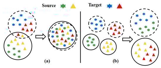
Figure 1. Results of different methods on domain adaptation problem. (a) target domain adaptation based on global domain adaptation method; (b) target domains adaptation based on related subdomain adaptation method.

Aiming to mitigate said deficiencies, the authors proposed a bearing fault diagnosis model based on the deep subdomain adaptive split attention network (SPDSAN). This method extracts the signal features through the residual network fused with multipath and channel attention mechanisms. Next, local maximum mean discrepancy (LMMD) is used to align distributions of related subdomains in two domains—as shown in Figure 1b. The scientific contributions of this paper are as follows:

• The vibration signal was transformed into a time-frequency graph by continuous wavelet transform as the learning object of the network. Compared with the one-dimensional vibration signal, the time-frequency graph can not only provide the time-domain and frequency-domain characteristics of the fault, but also avoid the network to learn the single dimensional characteristics and affect the diagnosis accuracy.
• The split attention module was introduced into the feature extraction network, and the multi-channel structure and attention mechanism were adopted to enrich the feature map diversity and improve the ability of the network to learn fault features.
• LMMD was used to measure the difference of relevant subdomains in the source domain and target domain data, and the distribution of relevant subdomains under the same category was adjusted to capture the fine-grained information of each category, so as to achieve the subdomain alignment.
• The method performance was compared to several widely used intelligent bearing fault diagnosis methods, and its effectiveness was verified.

2. Related Works

2.1. Problem Description

Transfer learning is applying the knowledge learned in the source domain as “experience” to the target domain, given that the source domain contains several labeled samples and meets the network training requirements. Samples in the target domain do not contain labels and are used as network final test sets. In this study, the source domain is the rolling bearing fault state signal collected under working condition A by laboratory simulation of the bearing fault. Furthermore, the target domain is the bearing fault state signal collected under working condition B. Let $D_s={\left\{\left(x_i^s,y_i^s\right)\right\}}_{i=1}^{n_s}$ be the data in the source domain, where $n_s$ is the number of fault samples in $D_s$, $x_i^s$ is the i-th sample in $D_s$, and $y_i^s$ is its corresponding fault label. Assuming that the health status of bearings has class $C$, and $y_{ij}^s=1,j=1,2,\cdots ,C$ indicates that the sample belongs to the j-th type fault. Further, $D_t={\left\{\left(x_j^t\right)\right\}}_{j=1}^{n_t}$ is the target domain, $n_t$ is the number of fault samples in $D_t$, and $x_j^t$ is the j-th sample in $D_t$. The probability distributions of $D_s$ and $D_t$ are denoted as $P$ and $Q$, respectively. It should be noted that $P\ne Q$.

2.2. ResNeSt-Split Attention Network

CNN has a strong ability to learn signal features. However, with the deepening of the network, the CNN gradient will disappear [22]. In 2015, He et al. [23] proposed ResNet residual neural network. Using the residual block structure combined with “Shortcut Connections”, the previous residual block can flow into the following block without obstruction. Thus, the problem of gradient disappearance caused by the network being too deep is avoided. Residual neural network (ResNet) used in this paper adds multiple split-attention (SA) block modules based on the ResNet. Moreover, residual split-attention networks (ResNeSt) combine the multipath structure with the channel attention mechanism, expressing the channel attention as a feature map group and weighting different branch feature channels to generate the final feature map (see Figure 2).

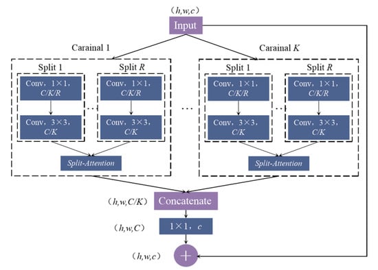
Figure 2. ResNeSt structure.

Firstly, the input feature map was divided into K branches, and each branch was subdivided into R subgroups. Hence, the total number of feature maps was $G=K\times R$. Secondly, $1\times 1,3\times 3$ convolution operation was carried out for each subgroup, and different weights were assigned to each subgroup through the SA module before it was finally aggregated. The feature map outputs obtained via aggregation and the residual module were combined linearly. Figure 3 shows the SA module.

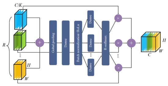
Figure 3. Split-attention module.

In the SA module, the combined feature ${\widehat{U}}^k$ of the k-th branch was obtained by element-wise summation and fusion of R subgroups:

$${\widehat{U}}^k={\displaystyle {\sum }_{j=R(k-1)+1}^{Rk}{U}_j},j\in 1,2,\cdots ,SK;k\in 1,2,\cdots ,K$$

(1)

where $U_j$ represents the j-th input feature in the SA module (the output feature after 3 × 3 convolution shown in Figure 3).

$${\widehat{U}}^k\in {ℝ}^{H\times W\times \frac{C}{K}},k\in 1,2,\cdots ,K$$

(2)

where H, W, and C/K represent the length, width, and the number of channels of each output feature map, respectively.

The global information obtained by global pooling of the fused feature maps was calculated next:

$$r_c^k=\frac{1}{H\times W}{\displaystyle {\sum }_{i=1}^H{\displaystyle {\sum }_{j=1}^W{\widehat{U}}_c^k}}\left(i,j\right)$$

(3)

where $r_c^k$ represents the c-th channel value of the 1 × 1 × C/K feature map of ${\widehat{U}}^k$ following the global pooling. Further, ${\widehat{U}}_c^k(i,j)$ represents the value at pixel (i,j) in the c-th channel of ${\widehat{U}}^k$.

Next, $r^k$ adaptively calculates the weight of each subgroup through the fully connected layer:

$$a_i^k\left(c\right)=\{\begin{array}{c}\frac{\exp (G_i^c(r^k))}{{\displaystyle {\sum }_{j=0}^{Rk}\exp (G_i^c(r^k))}}R>1\\ \frac{1}{1+\exp \left(-G_i^c(r^k)\right)}R=1\end{array}$$

(4)

where $a_i^k(c)$ is the weight of the i-th subgroup and $G_i^c$ is the weight function composed of two fully connected layers and a ReLU activation function.

Therefore, the final weighted fusion feature $V^k\in {ℝ}^{H\times W\times C}$ is generated by multiplying the original feature of each subgroup with the weight of each channel. The output of the c-th channel is as follows:

$$V_r{}^k={\displaystyle {\sum }_{i=1}^R{a}_i^k}(c)U_{R(k-1)+i},i\in 1,2,\cdots ,R$$

(5)

where $V_c^k$ represents the weighted fusion features of the c-th channel of each branch and $U_{S(k-1)+i}$ represents features of the $S(k-1)+i$-th subgroup.

2.3. Subdomain Adaptation

Maximum mean discrepancy (MMD) is widely used to evaluate the distribution difference between $D_s$ and $D_t$ [24]. However, using MMD to align the global distribution ignores the relationship between the source and the target domain’s relevant subdomains, losing each subclass’s fine-grained information. As such, it usually causes data confusion between both domains. Therefore, this paper introduced LMMD to align the distribution between the relevant subdomains. LMMD is expressed as:

$$d_{\mathscr{H}}\left(P,Q\right)\stackrel{△}{=}{\mathbb{E}}_c\Vert {\mathbb{E}}_{P^{(c)}}\left[\varphi (x^s)-{\mathbb{E}}_{Q^{(c)}}[\varphi (x^t)]\right]\Vert {}_{\mathscr{H}}^2$$

(6)

where $x_s$ and $x_t$ represent the sample instances in $D_s$ and $D_t$, respectively, $P$ and $Q$ are the distributions followed by these domains, $\parallel \cdot {\parallel }_{\mathscr{H}}$ is the regenerating kernel Hilbert space (RKHS), $\varphi (\cdot )$ is the mapping function, and $\mathbb{E}(\cdot )$ represents the mathematical expectation of the subclass. This paper introduces the concept of weights, which can be simplified as follows:

$$\{\begin{array}{l}{\stackrel{\wedge }{d}}_{\mathscr{H}}(P,Q)=\frac{1}{C}{\displaystyle \sum _{c=1}^C\Vert {\displaystyle \sum _{x_i\in D_s}{\omega }_i^{sc}}}\varphi (x_i^s)-{{\displaystyle \sum _{x_{j\in D_t}}{\omega }_j^{tc}\varphi (x_j^t)}\Vert }_{\mathscr{H}}^2\\ {\omega }_i^c=\frac{y_{ic}}{{\displaystyle {\sum }_{(x_j,y_j)\in D}{y}_{jc}}}\end{array}$$

(7)

where ${\omega }_i^{sc}$ and ${\omega }_j^{tc}$ are the weights of $x_i^s$ and $x_j^t$ belonging to subclass $c$, respectively. In this study, one-hot coding was used to calculate the weight $\omega$ of each sample belonging to the class. Further, $y_{ic}$ is the c-th element of the source-domain label vector $y_i$, representing the probability that the sample belongs to class $c$. For target domain samples without labels, the pseudo-label $y_j^t$ output by the SoftMax was used to calculate the weight ${\omega }_i^{tc}$ of sample $x_i^t$ belonging to class $c$. Finally, the SPDSAN will generate activation functions in $l$ layer, namely ${\left\{z_i^{sl}\right\}}_{i=1}^{n_s}$ and ${\left\{z_j^{tl}\right\}}_{j=1}^{n_t}$ to achieve the deep network adaptation. Therefore, the subdomain adaptation function is:

$$\begin{array}{r}{\stackrel{\wedge }{d}}_{\mathscr{H}}(P,Q)=\frac{1}{C}{\displaystyle \sum _{c=1}^C[{\displaystyle \sum _{i=1}^{n_s}{\displaystyle \sum _{j=1}^{n_s}{\omega }_i^{sc}}}{\omega }_j^{sc}\mathcal{K}(z_i^{sl},z_j^{sl})}\\ +{\displaystyle \sum _{i=1}^{n_t}{\displaystyle \sum _{j=1}^{n_t}{\omega }_i^{tc}}}{\omega }_j^{tc}\mathcal{K}(z_i^{tl},z_j^{tl})\\ -2{\displaystyle \sum _{i=1}^{n_s}{\displaystyle \sum _{j=1}^{n_t}{\omega }_i^{sc}}}{\omega }_j^{sc}\mathcal{K}(z_i^{sl},z_j^{tl})]\end{array}$$

(8)

where $z^l$ denotes the $l$th $\left(l\in L=\left\{1,2,\cdots ,\left|L\right|\right\}\right)$ layer activation.

3. Method

3.1. The SPDSAN Diagnostic Process

The SPDSAN model process proposed in this paper is shown in Figure 4. It includes the time-frequency image generation, the domain-shared feature extractor, subdomain adaptation, and fault classification.

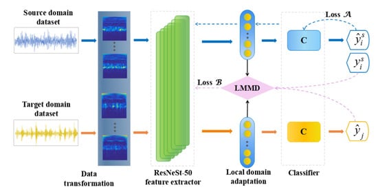
Figure 4. The structure diagram of the SPDSAN network model.

The diagnostic process was carried out as follows: firstly, the vibration signal was transformed into a time-frequency image as the network learning object. Secondly, the ResNeSt-50 was used to extract image signal features. By assigning different weights to channels, the ResNeSt-50 integrated channel attention mechanism improved the weight of fault features in the sample population, thus enabling, the network to learn more about the fault features in the sample. To reduce the training time and accelerate the model convergence, the ResNeSt-50 model was pre-trained using the ImageNet 2012 data for the general feature extraction. Then, the LMMD was used to measure the distribution differences of related subdomains in the subdomain adaptation layer, which was used as the optimization target $Lossℬ$ of the SPDSAN model. Finally, the error between the true $y_i^s$ of $D_s$ and the classifier-predicted label ${\widehat{y}}_i^s$ was assumed as the optimization objective $Loss\mathcal{A}$.

In sum, the training goal of the SPDSAN is to minimize $Loss\mathcal{A}$ and $Lossℬ$ to achieve higher diagnostic accuracy in the final diagnosis.

3.2. Target Optimization

The SPDSAN extracts the domain-transferable feature representations through deep feature representation learning and local maximum mean error learning. There are two optimization objectives in the training process:

• Minimizing the difference of $Loss\mathcal{A}$ between the real and the predicted label of the source domain sample. This will increase the classifier accuracy when diagnosing the source domain sample.
• Minimize the LMMD of $Lossℬ$ between the source and the target domain.

The $Loss\mathcal{A}$ can be expressed as:

$$Loss\mathcal{A}={\displaystyle \sum _{i=1}^{n_s}{J}_s}(f(x_i^s),y_i^s)$$

(9)

where $f(\cdot )$ is the predicted output of the source domain samples on the classifier and $J_s$ is the cross-entropy loss function.

The final optimization objective $J$ can be calculated as follows:

$$J=\min \frac{1}{n_s}Loss\mathcal{A}+\alpha Lossℬ$$

(10)

where $Lossℬ={\stackrel{\wedge }{d}}_{\mathscr{H}}(P,Q)$ and $\alpha$ is the trade-off parameter between the domain adaptation loss and the classifier loss.

4. Experiment and Analysis

All the presented experiments were completed using i7-9700K processor, 128 GB running memory, RTX 3070 TI graphics card, and Windows 10 operating system, while Pytorch was used as the code framework. The batch size of each training was 16, and the stochastic gradient descent algorithm was used for training. The momentum was 0.9, and the learning rate was ${\eta }_{\theta }=0.01/{\left(1+\alpha \theta \right)}^{\beta }$, where $\alpha =10,\beta =0.75$, and $\theta$ linearly changed from 0 to 1 during the training process [25].

4.1. Introduction to the Fault Datasets

The experimental data in this paper were collected from the bearing fault datasets of Case Western Reserve University (CWRU) [26] and the bearing model is SKF6205. The fault data acquisition test bench is shown in Figure 5.

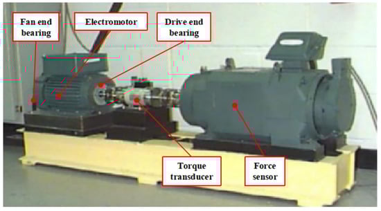
Figure 5. Data acquisition test bench.

The bearing dataset contains inner ring fault (IF), ball bearing fault (BF), and outer ring fault (BF) simulated by artificial electric discharge machining; the sampling frequency is 12 kHz. Each fault type contains three signals of different fault sizes (0.1778 mm, 0.3556 mm, 0.5334 mm). The details are shown in Table 1. In this study, four datasets (0, 1, 2, 3 HP) with different working conditions were generated to simulate the transfer learning tasks.

Table 1. Details of the CWRU dataset.

Serial Number	Healthy State	Fault Size/mm
NA	Normal	0
IF-0.1	Inner ring fault	0.1778
OF-0.1	Outer ring fault	0.1778
BF-0.1	Ball bearing fault	0.1778
IF-0.3	Inner ring fault	0.3556
OF-0.3	Outer ring fault	0.3556
BF-0.3	Ball bearing fault	0.3556
IF-0.5	Inner ring fault	0.5334
OF-0.5	Outer ring fault	0.5334
BF-0.5	Ball bearing fault	0.5334

4.2. Build Experimental Datasets

Continuous wavelet transform (CWT) is used to convert one-dimensional vibration signals into time-frequency graphs. Time-frequency graphs contain the time-domain and frequency-domain features of faults, which can avoid the influence of single feature of network learning on diagnostic accuracy. Therefore, in this study, the continuous wavelet transform was used to convert the vibration signal into a two-dimensional time-frequency image as the input of the network [27].

Firstly, in order to expand the number of datasets, an overlapping sampling technique was employed in each health condition dataset [28]. As shown in the Figure 6, the original vibration signal is sliced with a window of 1024 points, and each data sample contains 1024 points. Then, CWT was used to convert the selected 1024 points into a time-frequency image with a size of 256 × 256, the wavelet base was selected as cmor3-3, and the size sequence length was 64. In addition, another 1024 continuous sampling points were selected in the way of overlapping sampling to generate another time-frequency image; each sample overlaps 500 points.

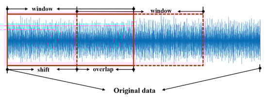
Figure 6. Data argument with overlap.

The number of obtained health status samples is shown in Table 2. The 10 health states under four different loads were alternately used as $D_s$ and $D_t$ for learning and transfer. Samples in the $D_t$ were not labeled during the network learning process to represent different fault samples under unknown working conditions.

For example, in the task “Working condition 0-1”, 10 types of health status data under 0 HP load were used as source domain samples, and another 10 under 1 HP load were used as target domain samples for the transfer learning task.

Table 2. The CWRU sample size scale.

Healthy State	Fault Size	0 HP	1 HP	2 HP	3 HP	All
NA	0	486	966	968	968	3388
	0.1778	241	242	243	244	970
IF	0.3556	242	242	242	242	968
	0.5334	243	242	242	242	969
	0.1778	242	243	241	244	970
OF	0.3556	242	242	242	242	968
	0.5334	243	242	243	242	970
	0.1778	244	241	242	242	969
BF	0.3556	242	243	242	243	970
	0.5334	242	242	243	243	970
All	----	2667	3145	3148	3152	12,112

Table 2. The CWRU sample size scale.

Healthy State	Fault Size	0 HP	1 HP	2 HP	3 HP	All
NA	0	486	966	968	968	3388
	0.1778	241	242	243	244	970
IF	0.3556	242	242	242	242	968
	0.5334	243	242	242	242	969
	0.1778	242	243	241	244	970
OF	0.3556	242	242	242	242	968
	0.5334	243	242	243	242	970
	0.1778	244	241	242	242	969
BF	0.3556	242	243	242	243	970
	0.5334	242	242	243	243	970
All	----	2667	3145	3148	3152	12,112

4.3. The Experimental Contrast

In this paper, four widely cited methods were selected for comparative experiments. These included deep adaptation network (DAN) [29], dynamic adversarial adaption network (DAAN) [30], multi-feature representation adaption network (MRAN) [31], and deep subdomain adaptation network methods with ResNet-50 as a feature extractor (RDSAN).

The input of the selected comparison method is a time-frequency image with a pixel value of 246 px × 246 px. The same feature extractor (ResNeSt-50) is used for DAN, DAAN, and MRAN to ensure that the experimental comparison would be valid. The experimental results are shown in Table 3. The average diagnostic accuracy of the proposed method in 12 migration tasks is 99.9%, which is higher than the accuracy obtained using other diagnostic models.

Table 3. Diagnostic accuracy of different models (%).

Methods/Task	0-1	0-2	0-3	1-0	1-2	1-3	2-0	2-1	2-3	3-0	3-1	3-2	Average
DAN	95.2	99.0	95.6	90.2	96.6	96.3	88.0	93.4	98.8	84.0	90.3	91.5	93.2
DAAN	98.0	97.0	92.0	89.0	99.0	96.0	82.0	93.0	89.0	85.0	82.0	97.0	91.6
MRAN	99.0	100	99.0	94.0	100	99.0	100	99.0	100	97.0	99.0	100	98.8
RDSAN	99.5	99.9	99.8	99.7	100	99.9	99.7	99.3	100	90.5	99.2	100	98.9
SPDSAN	100	100	99.9	99.9	100	99.9	99.9	99.4	99.9	99.5	99.8	100	99.9

Combining Table 3 and Figure 7 shows that the DAN adopts global alignment, with an average diagnostic accuracy of 91.5%. However, the diagnostic accuracy of each task fluctuates greatly, especially for task 2-0 (only 88%). The reason for such behavior is that global adaptation aims to align the overall distribution of the $D_s$ and the $D_t$; thus, the correlation between each subfield is ignored. The DAAN has the weakest recognition effect, with an average diagnostic accuracy of 91.6%. The recognition accuracy fluctuates greatly, and its robustness is the lowest. This is due to the global alignment that is based on adversarial thinking, requiring a large sample set of $D_s$ and $D_t$ to confuse the domain discriminator, making it unable to judge the sample domain label to achieve the global alignment. Therefore, using too few samples is the main reason for its low diagnostic accuracy.

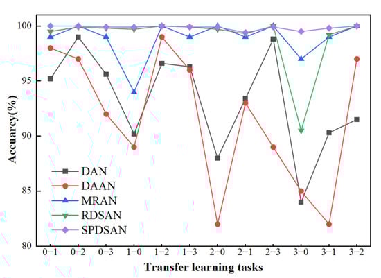
Figure 7. Diagnostic accuracy of the CWRU dataset.

The MRAN makes up for the DAN defect by extracting multi-representation features of sample images and aligning them in different feature spaces. However, the diagnostic accuracy in task 1-0 is only 94%. The primary reason is that when the samples of the $D_s$ and the $D_t$ have high similarity, the extracted multi-representation features are more similar. Hence, they cannot be classified correctly, yielding an average diagnostic accuracy of 98.8%.

Under the premise of using the subdomain migration method, the average diagnostic accuracy of RDSAN using Resnet-50 as a feature extractor is 98.8%. This value is lower than 99.9% obtained for the SPDSAN, proving that the SPDSAN has a stronger ability to learn fault features.

4.4. Feature Visualization

In this paper, the t-distribution random adjacent embedding algorithm [32] was used to visualize the data features of the $D_t$ of 12 transfer learning tasks and present them in the form of scatter plots, as shown in Figure 8 and Figure 9.

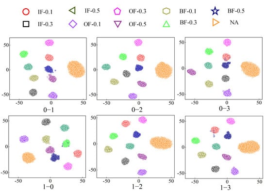
Figure 8. Feature visualization 1.

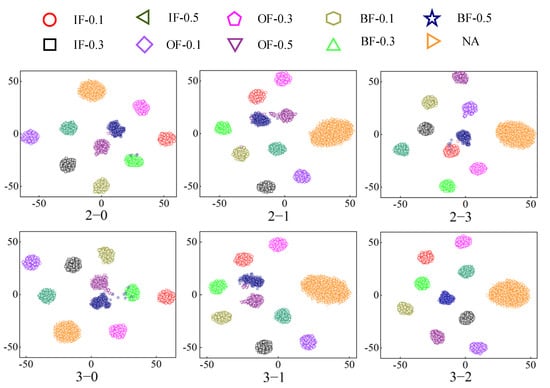
Figure 9. Feature visualization 2.

Each subfigure in Figure 7 and Figure 8 contains 10 health states. Different shapes and colors represent one health status. It is evident from clustering results that each health state can be well clustered with distinct regional characteristics through the adaptive alignment of subdomains. However, in part of the migration task, the 0.5334 mm ball fault was mistakenly assigned to other health states. This may be due to the signal characteristics of the fault, which are similar to those of other health states in different periods. Hence, the diagnosis accuracy of the migration as mentioned above task is slightly lower than that of other migration tasks.

5. Conclusions

To address the inconsistency in feature extraction network problems when applied to bearing fault diagnosis, such as insufficient ability to learn fault features and the characteristic distribution of vibration data of rolling bearing collected under variable working conditions, the authors proposed the SPDSAN diagnostic model. The experimental results have shown that the proposed model has higher robustness and diagnostic accuracy compared to other methods. Based on the results, the following conclusions can be made:

• Compared with ResNet, ResNeSt, which integrates multi-channel and split-attention mechanisms, can more fully learn the transferable fault features in samples. This facilitates subsequent transfer learning tasks.
• In the domain adaptation layer, the subdomain alignment method is used to reduce the distribution difference between the $D_s$ and the $D_t$, and to reduce the misdiagnosis caused by the small subdomain distance caused by the global alignment. Therefore, it is only necessary to train the network with samples under one working condition to complete the fault diagnosis under all working conditions
• The comparison and analysis of different experimental results show that the proposed method has good generalization and robustness.

References

- Qin, Y.F.; Shi, X.J. Fault Diagnosis Method for Rolling Bearings Based on Two-Channel CNN under Unbalanced Datasets. Appl. Sci. 2022, 12, 8474. [Google Scholar] [CrossRef]
- George, G.; Theodore, L.; Chrysostomos, D.S.; Vassilis, K. Bearing fault detection based on hybrid ensemble detector and empirical mode decomposition. Mech. Syst. Signal Process. 2013, 41, 510–525. [Google Scholar] [CrossRef]
- Ambrożkiewicz, B.; Litak, G.; Georgiadis, A.; Meier, N.; Gassner, A. Analysis of Dynamic Response of a Two Degrees of Freedom (2-DOF) Ball Bearing Nonlinear Model. Appl. Sci. 2021, 11, 787. [Google Scholar] [CrossRef]
- Huang, F.Y.F.; Chen, K.K.; Ma, H.; Li, X.; Han, H.Z.; Zhao, Z.F. Meshing and dynamic characteristics analysis of spalled gear systems: A theoretical and experimental study. Mech. Syst. Signal Process. 2020, 139, 106640. [Google Scholar] [CrossRef]
- Hu, B.Q.; Liu, J.; Zhao, R.Z.; Xu, Y.; Huo, T.L. A New Fault Diagnosis Method for Unbalanced Data Based on 1DCNN and L2-SVM. Appl. Sci. 2022, 12, 9880. [Google Scholar] [CrossRef]
- Arkadiusz, S.; Jacek, C.; Piotr, J. Detection of cylinder misfire in an aircraft engine using linear and non-linear signal analysis. Measurement 2021, 174, 108982. [Google Scholar] [CrossRef]
- Wang, H.T.; Guo, Y.Q.; Shi, L.C.; Pu, L.D.; Nie, Y.W.; Wu, W. Mathematical Problems in Engineering Research on Composite Fault Separation of Rolling Bearing Based on Functional Mixing Decoupling Model. Math. Probl. Eng. 2022, 2022, 9037709. [Google Scholar] [CrossRef]
- Almounajjed, A.; Sahoo, A.K.; Kumar, M.K. Diagnosis of stator fault severity in induction motor based on discrete wavelet analysis. Measurement 2021, 182, 109780. [Google Scholar] [CrossRef]
- Wu, J.; Guo, P.F.; Cheng, Y.W.; Zhu, H.P.; Wang, X.B.; Shao, X.Y. Ensemble Generalized Multiclass Support-Vector-Machine-Based Health Evaluation of Complex Degradation Systems. IEEE/ASME Trans. Mechatron. 2020, 25, 2230–2240. [Google Scholar] [CrossRef]
- Li, X.; Yang, Y.; Pan, H.Y.; Cheng, J.; Cheng, J.S. Non-parallelleast squares support matrix machine for rolling bearing fault diagnosis. Mech. Mach. Theory 2020, 145, 103676. [Google Scholar] [CrossRef]
- Sharanya, S.; Venkataraman, R. An intelligent Context Based Multi-layered Bayesian Inferential predictive analytic framework for classifying machine states. J. Ambient. Intell. Humaniz. Comput. 2020, 12, 7353–7361. [Google Scholar] [CrossRef]
- Vyas, N.S.; Satishkumar, D. Artificial neural network design for fault identification in a rotor-bearing system. Mech. Mach. Theory 2000, 36, 157–175. [Google Scholar] [CrossRef]
- Lei, Y.G.; Jia, F.; Lin, J.; Xing, S.B.; Ding, S.X. An Intelligent Fault Diagnosis Method Using Unsupervised Feature Learning Towards Mechanical Big Data. IEEE Trans. Ind. Electron. 2016, 63, 3137–3147. [Google Scholar] [CrossRef]
- Chen, Z.Y.; Wang, Y.Z.; Wu, J.; Deng, C.; Hu, K. Sensor data-driven structural damage detection based on deep convolutional neural networks and continuous wavelet transform. Appl. Intell. 2021, 51, 5598–5609. [Google Scholar] [CrossRef]
- Wang, N.N.; Ma, P.; Zhang, H.L.; Wang, C. Fault diagnosis of rolling bearings based on multi-scale deep convolutional network feature fusion. China J. Sol. Energy 2022, 43, 351–358. [Google Scholar] [CrossRef]
- Wu, Y.C.; Zhao, R.Z.; Jin, W.Y.; Xing, Z.Y. Fault Identification Method Based on Convolutional Neural Network for Data Imbalance. China Vib. Test Diagn. 2022, 42, 299–307, 408. [Google Scholar] [CrossRef]
- Wang, Q.; Deng, L.F.; Zhao, R.Z. Based on improved one-dimensional convolutional neural networks of the rolling bearing fault recognition. China J. Vib. Shock. 2022, 9, 216–223. [Google Scholar] [CrossRef]
- Yang, B.; Lei, Y.G.; Jia, F.; Xing, S.B. An intelligent fault diagnosis approach based on transfer learning from laboratory bearings to locomotive bearings. Mech. Syst. Signal Process. 2019, 122, 692–706. [Google Scholar] [CrossRef]
- Yang, B.; Lei, Y.H.; Jia, F.; Li, N.P.; Du, Z.J. A Polynomial Kernel Induced Distance Metric to Improve Deep Transfer Learning for Fault Diagnosis of Machines. IEEE Trans. Ind. Electron. 2019, 67, 9747–9757. [Google Scholar] [CrossRef]
- Chen, Z.Y.; Zhong, Q.; Huang, R.Y.; Liao, Y.X.; Li, J.P.; Li, W.H. Mechanical Intelligent fault Diagnosis based on Enhanced Migration Convolutional Neural Network. China J. Mech. Eng. 2021, 57, 96–105. [Google Scholar] [CrossRef]
- Cheng, C.; Zhou, B.T.; Ma, G.J.; Wu, D.R.; Yuan, Y. Wasserstein distance based deep adversarial transfer learning for intelligent fault diagnosis with unlabeled or insufficient labeled data. Neurocomputing 2020, 409, 35–45. [Google Scholar] [CrossRef]
- Gai, J.X.; Xue, X.F.; Wu, J.Y.; Nan, R.X. Cooperative spectrum sensing method based on deep convolutional neural network. China J. Electron. Inf. Technol. 2021, 43, 2911–2919. [Google Scholar] [CrossRef]
- He, K.M.; Zhang, X.Y.; Ren, S.Q.; Jian, S. Deep Residual Learning for Image Recognition. CoRR 2016, 12, 770–778. [Google Scholar] [CrossRef]
- Pan, Y.B.; Hong, R.J.; Chen, J.; Feng, J.S.; Wu, W.W. Performance degradation assessment of wind turbine gearbox based on maximum mean discrepancy and multi-sensor transfer learning. Struct. Health Monit. 2021, 20, 118–138. [Google Scholar] [CrossRef]
- Yaroslav, G.; Victor, S.L. Unsupervised Domain Adaptation by Backpropagation. CoRR 2014, 37, 1180–1189. [Google Scholar] [CrossRef]
- Case Western Reserve University Bearing Data Center Website. Available online: https://engineering.case.edu/bearingdatacenter/download-data-file (accessed on 1 April 2022).
- Zhang, L.; Liu, Y.Y.; Zhou, J.M.; Luo, M.X.; Pu, S.X.; Yang, X.T. An Imbalanced Fault Diagnosis Method Based on TFFO and CNN for Rotating Machinery. Sensors 2022, 22, 8749. [Google Scholar] [CrossRef]
- Li, Q.; Huang, Q.Y.; Yang, T.; Zhou, Y.; Yang, K.; Song, H. Internal defects inspection of arc magnets using multi-head attention-based CNN. Measurement 2022, 202, 111808. [Google Scholar] [CrossRef]
- Long, M.S.; Wang, J.M. Learning Transferable Features with Deep Adaptation Networks. CoRR 2015, 37, 97–105. [Google Scholar] [CrossRef]
- Yu, C.H.; Wang, J.D.; Chen, Y.Q.; Huang, M.Y. Transfer Learning with Dynamic Adversarial Adaptation Network. CoRR 2019, 38, 778–786. [Google Scholar] [CrossRef]
- Zhu, Y.C.; Zhuang, F.Z.; Wang, J.D.; Chen, J.W.; Shi, Z.P.; Wu, W.J.; He, Q. Multi-representation adaptation network for cross-domain image classification. Neural Netw. 2019, 119, 214–221. [Google Scholar] [CrossRef]
- Laurens, V.D.M.; Geoffrey, H. Visualizing Data using t-SNE. J. Mach. Learn. Res. 2008, 9, 2579–2605. [Google Scholar]
Publisher’s Note: MDPI stays neutral with regard to jurisdictional claims in published maps and institutional affiliations. |
© 2022 by the authors. Licensee MDPI, Basel, Switzerland. This article is an open access article distributed under the terms and conditions of the Creative Commons Attribution (CC BY) license (https://creativecommons.org/licenses/by/4.0/).