An Optimized Gradient Boost Decision Tree Using Enhanced African Buffalo Optimization Method for Cyber Security Intrusion Detection

Abstract

The cyber security field has witnessed several intrusion detection systems (IDSs) that are critical to the detection of malicious activities in network traffic. In the last couple of years, much research has been conducted in this field; however, in the present circumstances, network attacks are increasing in both volume and diverseness. The objective of this research work is to introduce new IDSs based on a combination of Genetic Algorithms (GAs) and Optimized Gradient Boost Decision Trees (OGBDTs). To improve classification, enhanced African Buffalo Optimizations (EABOs) are used. Optimization Gradient Boost Decision Trees (OGBDT-IDS) include data exploration, preprocessing, standardization, and feature ratings/selection modules. In high-dimensional data, GAs are appropriate tools for selecting features. In machine learning techniques (MLTs), gradient-boosted decision trees (GBDTs) are used as a base learner, and the predictions are added to the set of trees. In this study, the experimental results demonstrate that the proposed methods improve cyber intrusion detection for unused and new cases. Based on performance evaluations, the proposed IDS (OGBDT) performs better than traditional MLTs. The performances are evaluated by comparing accuracy, precision, recall, and F-score using the UNBS-NB 15, KDD 99, and CICIDS2018 datasets. The proposed IDS has the highest attack detection rates, and can predict attacks in all datasets in the least amount of time.

1. Introduction

Recently, the need for cybersecurity and protective measures against cyberattacks has increased. Cyberattacks are typically criminal activities launched over the Internet. Cyberattacks include theft of corporate intellectual property, theft of online bank accounts, creation and distribution of malware on systems, disclosure of valuable corporate information through public media such as the Internet, and disruption of countries’ critical infrastructure. Thefts or losses of data or information are very serious consequences of cyber-attacks worldwide [1]. In order to learn more, cyber threats should be studied proactively, and the experiences of other organizations affected by cyber-attacks should be shared [2].

In both the education and digital industries, especially small and medium enterprises (SMEs), online and computer networks are increasingly exposed to extremely complex cyber threats, resulting in financial losses [3]. Therefore, the research and development of cybersecurity technologies are important for IDSs to establish the first lines of defense, in order to prevent and respond to intrusion threats when new security issues arise. The development of data-driven intelligent IDS can analyze various patterns of cyber events, and then predict threats based on the examined data. Therefore, artificial intelligence (AI) expertise that uses MLTs to learn from security datasets can play a critical role in mitigating these threats. In the area of predictive analytics, tree-based strategies perform better in MLTs [4].

Modern security datasets contain rich features and dimensions in terms of security properties, with many irrelevant features that add to the complexity of efficient cyberattack modeling. These additional features also form the basis for several problems, such as increased variances, leading to overfitting of data in tree-based models that learn decisions based on single paths; an increase in computation and execution time of training models; and a lack of model generalization [5,6,7,8]. This leads to a lower prediction accuracy of attack detection rate. One of the most accurate metrics scores, the accuracy score, illustrates how effectively the model generates correct forecasts in general.

Therefore, the main goal of this work is to minimize the security problems described above and to develop efficient data-driven IDS for cybersecurity. To achieve this goal, this work proposed OGBDT-IDS based on MLTs for network security. The proposed scheme helps to mitigate the above problems. First, the security features are ranked according to their modeling relevance, and then a tree-based generalized IDS is constructed based on the selected relevant features using GAs. Model validation of the OGBDT trees created in training is performed using test data. By reducing overlap in modeling, the computational complexity of the proposed model is reduced by dimensionality reduction before generating the results. The proposed scheme is ideal for the improved prediction of new and not-found cases.

The contributions of this research are listed below:

• For high-dimensional data, MLTs are proposed as a method for ranking the importance of security attributes using Gini indices.
• OGBDT-IDS is a network security technique based on MLTs that produces trees using derived attribute ranks and selects important features using GAs.
• To maximize the predictive power of the GBDT models, an OGBDT is created based on the selected significant attributes. Hyperparameters can be tuned manually or by automated methods, such as those based on EABOs.
• The proposed IDS (OGBDT-IDS) is then evaluated through experiments. The experimental results of this study with test data show that the proposed methods improve cyber intrusion detection for new and unused cases.

The performance of the proposed OGBDT-IDS is compared with the existing one given in the literature [6,7,8,9,10,11], for validation reasons. OGBDTs perform better than all other models in terms of accuracy. In all datasets, OGBDTs can predict attacks in the least amount of time. By simultaneously optimizing GBDTs and improving classification results, the proposed OGBDTs framework can significantly improve cyber-attack classification performance.

After this introductory section, Section 2 describes the background and relevant work on IDSs. Section 3 describes the tree structures used in MLTs for IDSs and the proposed OGBDT-IDS. Section 4 explains the performance evaluation of the final security model and examines the results of experiments conducted on the cybersecurity dataset. Finally, Section 5 concludes this paper and analyzes the planned future work.

2. Related Work

The growing demands for strong and effective IDS have sparked the interest of academic researchers in suspicious activity detection and cyberattacks. MLTs have the potential to play an important role in the development of intelligent and effective IDSs. Recent MLT approaches proposed to predict attacks on communication networks are based on tree-based approaches [12].

Rahouti et al. [13] and Babiker Mohamed et al. [14] proposed an integrated approach that combines two methods: “security with SDN” and “security for SDN”, to better protect globally connected Internet networks from cyberattacks. Sarker et al. [15] proposed a behavior-based method based on DTs (decision trees) to predict user actions in multidimensional environments. Gifty et al. [16] focused on the security and privacy management of CPS, and proposed a reliable IDS with reduced failures for Big Data environments. Improved predictive algorithms to efficiently identify attacks in a given network have also been the focus of several research papers.

Puthran and Shah [17] focused on the poor performance of the ID3 algorithm for Probe, R2L, and U2R attacks. Their model was developed to increase the prediction accuracy while keeping the processing complexity to a minimum (i.e., adaptations and execution times). The goal of this research was to raise awareness of this issue by analyzing the risks associated with DMPC techniques and reviewing defense strategies. Several examples are given at the end to show the way these defense strategies are implemented in DMPC controllers [18]. However, this only shows the development of simple rules. Sarkar [19] proposed Cyber Learning based on binary classifications where anomalies were identified, while their multi-class classifications could detect cyber-attack types.

A study by Reference [20] found that 142 papers between 2010 and 2015 used the KDD99 dataset. The dataset includes five classes (Normal, DoS, Probe, Remote-to-Local (R2L), and User-to-Root) and 41 features (excluding the labels) (U2R). The training and testing sets of the KDD99 [21] contain 494,021 and 311,029 records, respectively. The DoS class holds the most records, followed by the Normal class. Furthermore, there are more entries classed as R2L in the testing set. Numerous duplicate records were discovered in this set of records.

The freely accessible UNSW-NB15 dataset [22] consists of 42 features and ten classes (Normal, Fuzzers, Analysis, Backdoors, DoS, Exploits, Generic, Reconnaissance, Shellcode, and Worms) (not including the labels). Its testing set contains 82,332 records, while its training set contains 175,341 records. Unevenness also exists in the UNSW-training NB15 classes and test sets.

CSE-CIC-IDS2018 [23] is the most recent and realistic cyber dataset from the Canadian Establishment for Cybersecurity (CICmost). CIC and ISCX datasets are used globally for malware identification and intrusion detection. The primary objective of this dataset is to develop a methodological framework for handling the generation of diverse and comprehensive benchmark datasets, for the purpose of intrusion detection on the generation of client profiles, which contain theoretical representations of actions and behaviors carried out on the system. The dataset comprises the captures, structured traffic, and system logs of each machine, as well as 80 highlights that were taken from the traffic recorded using CICFlowMeter-V3.Java code, which was used to create CICFlowMeter-V3, a network traffic flow generator with good control over the features and time flow duration. This particular dataset is prepared as a CSV document containing six key features—SourceIP, FlowID, DestinationIP, DestinationPort, and SourcePort—and 80 features designated as Protocol [9]. Intrusion detection in the internet of things is performed using the supervised machine learning algorithm and the UNSW-NB15 dataset discussed in [10].

Utilizing KDD99 Data and the UNSW-NB 15 Dataset with a gradient-boosted machine, anomaly detection was conducted [11]. The first step in developing the security framework was to apply common MLTs, including NBs (naïve Bayes), LRs (logistic regressions), SGDs (stochastic gradient descents), KNNs (K-nearest neighbors), SVMs (support vector machines), DTs, RFs (random forests), adaptive boosting, extreme gradient boosting, and LD ||As (linear discriminant analyses). Subsequently, a security architecture based on ANNs (artificial neural networks) has also been included, which takes into account numerous hidden layers.

A new approach iReTADS was proposed in [24] to increase network security, while reducing network traffic by leveraging a potent real-time neural network for data summarization. Although data summarizing is a crucial part of data mining, there are no reliable ways to evaluate the summary at the moment. The goal of Li and Liu’s study in [25] was to explore the challenges, drawbacks, and benefits of the proposed approaches by examining and thoroughly analyzing cybersecurity developments. Jahromi et al. [26] described two-stage attack detection and attribution models which they developed for CPS, and specifically for ICS (industrial control systems). First, DTs were integrated with new Ensemble Deep Representation Learning models to detect attacks in unbalanced scenarios of ICS. In the next phase, Ensemble Deep Neural Networks (DNNs) were used to characterize attacks. The proposed model was tested on practical datasets of gas pipelines and water treatment systems.

Zhang et al. [27] proposed a technique for detecting attacks on cyber-physical systems. In their work, KNNs, DTs, bootstrap aggregations or bagging, and RFs were studied as classification models. In their proposed study, an auto-associative kernel regression model was used to improve the timely detection of attacks. Although the proposals were accurate, due to technical issues, their results were not sufficient. To predict attacks in virtual networks, Sedjelmaci et al. [28] developed Bayesian game theory IDS to prevent and predict future activities of monitored vehicles.

Cui et al. [29] proposed attack detection modules relying on Hilbert–Huang transforms and DLTs to detect attacks on DCs (direct current networks), MGs (microgrids), and DGs (distributed power generations). Their KHOs (Krill Swarm Optimizations) were a DLT for current election groups. DTs can play an important role in the development of IDS; however, these systems must handle large amounts of network traffic with multidimensional data, while being resilient and effective, and also reducing computational complexity with increased accuracy in their detection processes.

The African Buffalo Optimal Decision Tree (ABODT) is an algorithm proposed by Panhalkar, A.R., and Doye, D.D. [30] that uses the intelligent and social behavior of African buffalos to generate globally optimized decision trees. In order to use the African buffalo optimization (ABO) method as an optimizer to change the weights of the probabilistic neural network, Alweshah, M. et al. [31] suggested a hybridization strategy (PNN). It is critical to limit the number of input variables so as to reduce the computational cost of modeling and improve model performance in certain cases. A decision tree is a classification technique that can help in knowledge extraction from a database. When there are more features and instances, databases grow tremendously quickly and accumulate much data. Although decision trees have several issues, their key drawbacks are instability, local judgments, and overfitting for this enormous amount of data.

3. Research Methodology

Data exploration, preprocessing and standardization, and ranking and selection are the three key components of the proposed OGBTD IDS. These stages are necessary to develop tree-based IDS methods that select features based on ranks. In the final two modules, the data are trained and put to the test to determine how effectively it can categorize cyberattacks. Figure 1 shows the suggested framework, and the following sections evaluate each stage of the model in more detail.

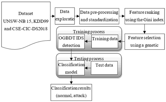
Figure 1. An optimized gradient boost decision trees-based IDSs model.

3.1. Input Dataset and Data Exploration

Data quality is one of the most important factors for the prediction accuracy of the proposed predictive models in data mining methods. Therefore, in this framework, the data are explored in the step of data exploration to learn more about their characteristics and evaluate the data integrity, and the data are cleaned. In addition, the features are explored to find their data types, namely numeric or categorical. The dataset in this study is from UNSW-NB 15 [21], KDD99 [22], and CSE-CIC-DS2018 [23]. The dataset UNSW-NB 15 was developed at the Australian Centre for Cybersecurity’s Cyber Range Lab, and contains 42 features, including attack data. The class features of the dataset define whether the activities are normal or attacks. The attack type attribute was not included in this research, because it did not fit within the scope of this study. After data exploration, 42 features were selected, and the attributes were quantitative, except for the service, proto, and state attributes. The KDD 99 dataset contained 41 attributes, of which three (protocol type, service, and latency) were qualitative and the rest were quantitative [20]. Seven different attack scenarios, including brute force, botnet, denial of service, distributed denial of service, online attacks, and network infiltration, are included in the CSE-CIC-DS2018 dataset. After data exploration, 41 features were selected from the raw network data.

3.2. Steps in Data Preprocessing and Standardization

This section includes checking the presence of input features that are redundant in the datasets, translating the available nominal input features into the numerical form, mapping them to the same scale, extracting the most useful input features to prevent the features from biasing the classification results, and reducing the computational burden during the visualization phase [20]. The mapping of input features to the same scale was performed using six algorithmic data transformations, namely normalizers, scalers (Min-Max, Robust, and Standard), and transformers (Quantile and Power), along with their suitability for numerical inputs. In the earlier section, the nominal security features whose encoding was to be performed were recognized, including Proto, Service, and State. Two techniques (encodings) can be used in this context. The use of label encoding was chosen instead of One Hot Encoding because the number of nominal security features is increased when One Hot Encoding is used. All feature values are converted to numeric values using the Label Encoding method [32,33]. The following step refers to features with different value distributions or scales that are not similar. This technique is considered important for data preprocessing, and should be completed before tree-based IDSs process the data. All features in the dataset that have a significant variation in the scale of the data are rescaled, so that the values for each feature F represent a mean of zero with a variance of one.

$$F_{newscale}=\frac{F_{original}-\overline{F}}{\sigma }$$

(1)

where $F_{newscale}$ denotes the feature’s new-scaled value, while $F_{original}$ denotes the feature’s original values, $F$ denotes the feature’s mean, and $\sigma$ denotes the standard deviation. All features are scaled, encoded, and ranked for the selection processes.

3.3. Features Ranking Using Gini Index

Supervised MLTs, such as DTs, require appropriate use of approaches to identify the most effective attributes that can impact decision-making processes. Two common approaches are generally considered for this purpose, namely information gains and Gini indices. The former indicates that features with maximum information gains are used as root nodes of DTs, while the latter specifies the features with the lowest GIs (Gini indices) for binary splits (decisions for nodes) [34]. In this work, ranks are added to features before evolving trees. Gini indices are added to the feature ranks to detect imprecision in the features. Gini indices are calculated by subtracting one from the sum of the squared probabilities of the classes. According to [35], GIs for characteristics (n) can be calculated using Equation (2).

$$GI\left(n\right)=1-{\displaystyle \sum }_{i=1}^c{\left(P_i\right)}^2$$

(2)

where $P_i$ denotes the likelihood of tuples in n that belong to separate security classes. This work uses threshold values (t = 0.02) for discovering the most relevant qualities of features in its suggested framework based on tree structures. It is important to realize that this number might change depending on the dataset in question.

3.4. Feature Selection Using a Genetic Algorithm

Here, the Genetic Algorithm [36] used is based on a feature selection method to select useful features. In the Genetic Algorithm, different combinations of features are called chromosomes, and every chromosome is be evaluated by the Fitness Function. According to the fitness value, only the highest-scored chromosome can survive to the next evolution round. The new chromosome replaces the old one in the total chromosome pool, which is called the initial population. When the evolutionary loop stops, relatively characteristic features are selected as an output of the Genetic Algorithm. Figure 2 illustrates the flowchart of the proposed feature selection process. The initial population consisted of feature chromosomes. Features in the dataset were coded into binary formations, such as 110110111…00101101. The chromosomes were generated randomly.

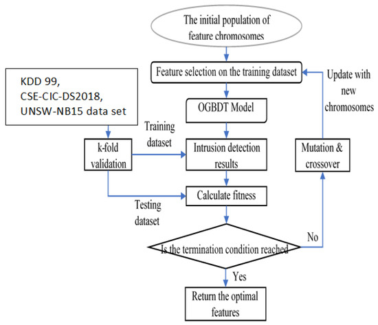
Figure 2. Flowchart of the proposed feature selection process.

However, to capture as many attack categories as possible in both datasets, the number of the initial population is limited to 100 to 150. From previous research, the larger the initial population, the more complex the algorithm, and the more computation time required. On the other hand, if the initial population is too small, the optimal performance of the algorithm is reduced, and it can easily slip into a local optimum. Both original datasets are split into training and test datasets, using K-fold validation during the training process. The mutation rate and crossover rate are kept constant in the experiments. Based on the classification results from RF, the fitness function evaluates each chromosome at the end of the iteration, and the feature extraction algorithm terminates when certain conditions are met. This occurs, e.g., when the highest number of specified iterations is reached, or when the search is complete and the maximum fitness values have not changed for 10 consecutive generations. At the end of each evolutionary step, the chromosome with the highest score by the fitness function replaces the chromosome with the lowest score.

A suitable fitness function should preserve chromosomes with high fitness values and speed up the iterative process of the genetic algorithm. Moreover, in IDS, not only the accuracy and true-positive rate, but also the false-positive rate should be included in the fitness functions. As a result, the number of features is reduced to 19, depending on the feature score. Figure 2 shows the features that will be used to build IDS frameworks based on tree architectures. The data are first prepared for processing using the proposed framework based on tree topologies. This work aims to reduce the computational complexity of building IDS frameworks based on tree architectures, and, thus, to improve their accuracy in terms of attack predictions, as the selected feature significantly affects the decision-making processes. The following section provides an overview of the evolution of tree-based IDS.

3.5. Proposed OGBDTs Cyber-Attack Detection

In this study, the combination of the gradient-boosting technique with EABOs is investigated in order to find the best set of hyperparameters to maximize the predictive performance of the cybersecurity model. Gradient-Boosted Decision Trees (GBDTS) trees are binary trees used in assigning label predictions to instances by performing thresholding on feature values. A decision tree t is initially specified as either a leaf that has a label prediction $\widehat{y}$ or a non-leaf node $\left(f,th,t_{left} ,t_{right}\right)$, where $f$ detects a feature, $th$ refers to the respective threshold, and $t_{left}$, $t_{right}$ specify the decision trees.

During the time of testing, the instance $\overrightarrow{x}$ performs tree $t$ traversal until it reaches the leaf, setting its prediction. Particularly, for every visited non-leaf node $\left(f ,th,t_{left} ,t_{right}\right)$, $\overrightarrow{x}$ is sorted into the left tree $t_{left}$ if $x_f\le th$; otherwise, it is sorted into the right tree $t_{right}$. With a training set $trainingset={\left\{{\overrightarrow{x}}_i,y_i\right\}}_i^n$, the conventional algorithms for decision tree learning initially predict the best label on $the training$ set for a decision tree consisting of one individual leaf, and later evaluate whether the loss can be reduced by substituting this leaf with a non-leaf node, resulting in two new leaves with predictions ${\widehat{y}}_{left}$, ${\widehat{y}}_{ right},$ correspondingly. The best substitute is achieved through an elaborate search of all the probable features $f$ and thresholds which are frequent in $the training set$. The predictions ${\widehat{y}}_{left}$, ${\widehat{y}}_{right}$ are calculated, which reduces the loss over $trainingse{t}_{left}=\{\left({\overrightarrow{x}}_i,y_i\right)\in trainingset|x_f\le th\}$ and $trainingse{t}_{right}=trainingset\backslash trainingse{t}_{left}$, correspondingly. The building recursively continues on the new leaves and terminates if the loss cannot be reduced further or if a certain stop condition is satisfied, e.g., the depth of the decision tree goes beyond a particular limit.

After the GA model has generated the optimum feature subset, data classification was carried out with the help of GBT. GBT was a boosting model, aiding in deriving an exact model with the baseline models included sequentially. The baseline models were trained at each stage of training to minimize the loss function. Friedman [37] developed the GBT model and fine-tuned generalized boosting models, employing DTs in both baseline models.

Formally, given a loss function $Loss$ and a dataset with $n$ instances and $f$ features ($trainingset=\left\{\left(x_i,y_i\right)\right\}\left(\left|trainingset=n,x_i\in I^d, y_i\in I\right|\right))$, GBDT minimizes the following objective function. Loss can be calculated using Equation (3).

$$\widetilde{Loss}={\displaystyle \sum }_{i}Loss\left({\widehat{y}}_i,y_i\right)+{\displaystyle \sum }_k\mathrm{Reg}\left(f_k\right)$$

(3)

where $Reg\left(f\right)=\gamma T_{loss}+\frac{1}{2}\lambda w^2$ refers to a regularization term to penalize the model complexity. Here, $\gamma$ and $\lambda$ are hyper-parameters, $T_{loss}$ indicates the number of leaves, and $w$ stands for the leaf weight. Each $f_k$ corresponds to a decision tree. Training the model in an additive manner, GBDT minimizes the following objective function at the $m$-th iteration. The GBT is initialized with a value $a_0$. A gradient descent process was used for every training process $m$ to minimize the loss function. Loss_min can be calculated using Equation (4).

$$Los{s}_{min}={\displaystyle \sum }_{i=1}^{n}Loss\left(y_i,f_{m-1}\left(x_i\right)+a_{m}bas{e}_m\left(x_i\right)\right)$$

(4)

DTs are built from the ground up until they hit certain constraints, such as the maximum depth. The 1st-order Taylor loss function’s expansions were calculated in training phases, and ${\mathfrak{F}}_{im}$ was calculated for finding the diminishing direction $a_{m}bas{e}_m\left(x_i\right)$. GBTs chose features with maximum information gain, such as the tree’s root node, where root nodes then distribute additional characteristics into child nodes with the next best information gain. Iterations of the division and addition processes resulted in new sets of grandchild nodes. The input space ($I$) was divided into $km$ joint regions $I_{1m},I_{2m},I_{jm},$ with estimated constant values of $c_{1m},c_{2m},c_{jm},$, correspondingly. The base learner $bas{e}_m\left(x\right)$ constitutes the total of these predicted values. In the next step, $a_{m}bas{e}_m\left(x_i\right)$ was chosen to minimize the loss function. At the end, the new model $f_m\left(x\right)$ was updated with the sum of $f\left(m-1\right)$ and $a_{m}bas{e}_m\left(x_i\right)$. However, the highest number of rounds leads to badly generalized models. To deal with this problem, Friedman’s algorithm uses a shrinkage variable $\mathcal{S}$ on the computed technique $a_{m}bas{e}_m\left(x_i\right),$ so that the learning rate of the training process is reduced. Further, the EABOs is used to optimize the hyperparameters of GBDT. $\gamma and \lambda$ are hyper-parameters, $T_{loss}$ refers to the number of leaves, and $w$ indicates the leaf weight.

Enhanced African Buffalo Optimization (EABOs)

The EABOs can be developed using the integration of the Discrete Crossover operators (DCOs) and African Buffalo Optimization (ABO) algorithms, with the special swap sequence operator SS principle, as shown in Algorithm 1.

Algorithm 1: Enhanced African buffalo optimization algorithm

Step 1: The population size (Pop size), the learning parameters L1 and L2, the maximum iterations count tmax, and the GBDT’s parameters, such as $\gamma , \lambda , T_{loss},$ $\mathrm{and} w,$ are set. EABOs evaluate the movements (arbitrary exploitation and exploration of buffalos, i.e., ${\alpha }_k$$\mathrm{and} {\beta }_k$), where the buffalos represent random parameter value vectors, and the characteristics can be chosen. Exploitations are substitutions made up of random sequences produced by the swap operator ($\widetilde{\mathbb{S}\mathbb{O}}$).   Step 2: Buffalo’s evaluations, wherein buffalos are assessed in terms of their objective function values, computed based on (Equation (3)).   Step 3: DCOs (discrete crossover operators): to ensure that the entire population moves towards global optimal solutions, DCOs [26] are incorporated to create a child from two parents using random real numbers. The offspring can be created by randomly selecting genes from both parents and distributing them evenly, depending on the random real number $r\in ⟨ 0,1 ⟩$. To produce new solutions, DCOs are applied between the global herd’s best solution $b_g$ and the present solutions ${\alpha }_k^t$ (i.e., child), resulting in ${\alpha }_{k-cross}^t$ as the solution.   Step 4: Updating exploitations: the initial buffalo’s exploitations ${\beta }_k^t$ consists of random swap operator sets $\widetilde{\mathbb{S}\mathbb{O},}$ which can be modified based on Equation (5). $${\beta }_k^{t+1}={\beta }_k^t\oplus L_1\otimes \left({\alpha }_{k-cross}^t-{\beta }_k^t\right)\oplus L_2\otimes \left(b_g^t-{\alpha }_k^t\right)$$ (5)   When referring to an integrating sequence operator that consists of two swap operators, the terms $L_1$ and $L_2$ specify the learning parameters with random values ranging between [0, 1], respectively. All swap operators can be selected from the swap sequence $\left({\alpha }_{k-cross}^t-{\beta }_k^t\right),$ and all swap operators can be selected from the swap sequence $\left(b_g^t-{\alpha }_k^t\right)$ which are provided as swap sequence operators $SS{O}_1$ and $SS{O}_2$, respectively. Therefore, we find ${\beta }_k^t=\left({\widetilde{\mathbb{S}\mathbb{O}}}_1,{\widetilde{\mathbb{S}\mathbb{O}}}_2,\dots ,{\widetilde{\mathbb{S}\mathbb{O}}}_s\right)$, where s signifies the number of swap operators in ${\beta }_k^t$, $SS{O}_1$ and $SS{O}_2$.   Step 5: The series of swap operators is applied on the existing solution to obtain a new solution, as well as a new movement, based on the present buffalo’s movement using Equation (6). $${\alpha }_k^{t+1}=\frac{\left({\alpha }_k^t+{\beta }_k^t\right)}{\mathfrak{u}}\forall k, k = \left\{1, \dots , Po{p}_{size}\right\}$$ (6) where u is a time interval initialized to 1 unit across the exploration motion.   Step 6: The global herd’s best solution, bg, is checked. Whether the best fitness value of the herd is updated or not is also checked; $if (b_{gmax}^t>b_g^t )$, then the process from step 2 must be repeated until the stop condition ${\max }_{iter}$ is satisfied. Otherwise, we eturn step one, and the procedure is repeated.   Step 7: The global best solution is obtained as the ultimate solution of hyperparameter values after a specific number of repetitions. Algorithm 1 explains the Enhanced African buffalo optimization method procedure.

Figure 3 shows an illustration of the tree structure-based framework in conjunction with penetrating OGBDTs, utilizing a depth of 3 or d = 3 to highlight the part of trees used for IDS that is determined by features. For instance, the branches of the tree were further expanded after the feature was still chosen as the root node based on the Gini indices. The decision nodes show the class names, the feature names, the Gini index, samples, and recorded values. The class name denotes whether a specific behavior is expected or hostile.

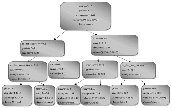
Figure 3. The tree structure-based framework (OGBDTs).

4. Experiment Results and Discussion

The datasets (KDD99, CSE-CIC-DS 2018, and UNSW-NB 15) used in this study were selected based on a variety of factors, including the number of samples, attributes, and classifications. TPs (true positives), FPs (false positives), TNs (true negatives), and FNs (false negatives) were all measured to calculate various performance measures. The first performance measure was precision, which is expressed as the percentage of applicable instances found. Recall, characterized as the percentage of relevant instances, was the second performance metric. Despite their often conflicting nature, the ratings of precision and recall are both critical to how effective a prediction strategy is. Therefore, these two measures can be added together and weighted equally to create the F-measure, a single metric. The accuracy measure, which was the final performance requirement, was defined as the percentage of events which were accurately predicted.

The proposed OGBTDS-IDS was evaluated using accuracies, precisions, recalls, and F-scores, and the results were compared using other traditional MLTs. Evaluating metrics for precisions (Equation (7)), recall (Equation (8)) F-measures (Equation (9)), and accuracy (Equation (10)) are given below.

$$\mathrm{Precision}=\frac{\mathrm{TP}}{\mathrm{TP}+\mathrm{FP}}\times 100$$

(7)

$$\mathrm{Recall}=\frac{\mathrm{TP}}{\mathrm{TP}+\mathrm{FN}}\times 100$$

(8)

$${\mathrm{F}}_{\mathrm{measure}}=2\ast \left(\frac{\mathrm{precision}\ast \mathrm{recall}}{\mathrm{precision}+\mathrm{recall}}\right)$$

(9)

$$\mathrm{Accuracy}=\frac{\mathrm{TP}+\mathrm{TN}}{\mathrm{TP}+\mathrm{FP}+\mathrm{TN}+\mathrm{FN}}\times 100$$

(10)

where TP is true positive, FP is false positive, TN is true negative, and FN is false negative.

Figure 4 compares the precision rates for the suggested and existing methods for identifying cyberattacks. The outcomes indicate that extracting the desired data can be accomplished by ranking the features using OGBDT. The number of usable features in the proposed model has little to no impact on how well the jointly learned feature transformation performs. Due to the lack of high-dimensional features or derived factors, an OGBDT may identify a comparatively better-sorted collection of inputs in a specified amount of time. The performance of the model was superior to all others, and KDD99 had a higher detection rate than the other two datasets.

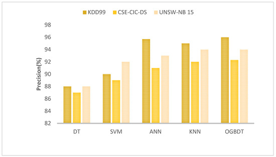
Figure 4. Precision rate comparison.

Recall rate comparison is shown in Figure 5 for proposed and existing models. An increased feature number maximizes recall as well. The OGBDTs achieve higher recall compared to DT, SVM, ANN, and KNN. This is because the EABOs save the computation time of the derived factors, which allows easier fine-tuning of the GBDT. Therefore, the proposed network can be safely used for intrusion detection.

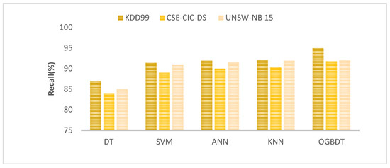
Figure 5. Recall rate comparison.

The f-measure for the number of features in the given databases for the proposed and current models is shown in Figure 6. The OGBDTs have a high f-measure compared to other models. EABOs use the parameters set with random values, and terminate when predefined stop conditions, such as maximum time, number of parameters, or performance target, are met. This avoids overfitting of the data, which is possible in real-time problems and leads to better performance.

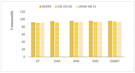
Figure 6. F-measure rate comparison.

Based on the number of features in the given databases, Figure 7 illustrates the accuracy of the proposed and existing models. As a result of OGBDTs, the processing time is reduced and accuracy is increased. The OGBDTs achieve higher accuracy compared to all other models because they do not require a large amount of derived factors during preprocessing. The proposed OGBDTs framework can significantly improve the performance of cyber-attack classification by jointly optimizing the GBDTs and improving the classification results.

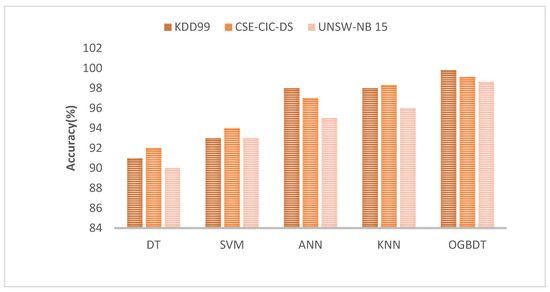
Figure 7. Accuracy comparison.

It can be observed from Figure 8 that the OGBDTs tree outperforms other models by taking the least time to train the framework compared to others. Each one of the approaches consumed much reduced time for training once the relevant attributes were eliminated. In all datasets, OGBDTs have a maximum accuracy rate to predict the attack.

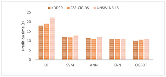
Figure 8. Prediction time comparison.

It can be observed from Figure 8 that the OGBDTs outperform other models by taking the least time to train the framework compared to others. Each one of the approaches significantly reduced the time for training once the relevant attributes were eliminated. In all datasets, OGBDTs have minimum time to predict the attack.

The results of the statistical metrics are as follows:

Accuracy: The accuracy score shows how effectively the model generates precise predictions in general. Among all the proposed models, OGBDT had the highest accuracy rate to predict the attack (0.9981). Out of all the datasets, OGBDTs had the greatest attack prediction accuracy rate. To obtain a more complete picture of the model’s performance, it is important to analyze it using various performance measure scores, such as Recall, Precision, and F1 SCORE.

Recall: Recall can be utilized as a metric to assess the efficacy of our model when all of the real values are positive, and OGBDT has a high recall rate for all of the datasets.

Precision: Compared to all other classifiers over the full dataset, OGBDT’s precision is high, and this actual value can be discriminated from all expected actual values.

F1 score: This metric can combine recall and precision by calculating its mean value, and it is also noticeably higher for OGBDT.

Prediction Time: OGBDTs outperform other models by taking the least time for training the framework, compared to others.

Evaluation criteria used to assess SVM, DT, K.N.N, ANN, and suggested OGBDT algorithms included sensitivity, specificity, accuracy, recall, and F1 score. These algorithms were tested using a binary classification method, and the performance of the algorithms was statistically quantified and compared to the body of existing literature [6,7,8,9,10,11] (Table 1) for validation purposes. The findings showed that the OBGDT algorithm was quite effective in identifying attacks. The performance of the suggested model was superior to all others. KDD99 had a higher detection rate than the other two datasets. The OGBDTs outperformed all other models in terms of accuracy, because they do not require as many derived factors during preprocessing. OGBDTs can forecast attacks with a minimum amount of time in all datasets. The proposed OGBDTs framework can significantly improve the performance of cyber-attack classification by jointly optimizing the GBDTs and improving the classification results.

Table 1. Results compared from similar studies.

Dataset Used	Machine Learning Algorithms	Attack Detection Rate ACCURACY
UNBS-NB 15 Dataset [10]	RF	0.9867
	SVM	0.9769
	ANN	0.9478
	DT	0.9323
KDD99 Dataset [8]	ANN	0.9744
	SVM	0.9155
	USML	0.9808
	DT	0.9333
UNBS-NB 15 Dataset [8]	ANN	0.6397
	SVM	0.8432
	USML	0.9478
	ANN	0.9744
	DT	0.9443
UNBS-NB 15 Dataset [7]	KNN	0.9611
	RF	0.9237
	XGBoost	0.9835
UNSW-NB 15 Dataset [6]	DT	0.9015
	ANN	0.8411
	Proposed approach GIWRF-DT	0.9301
KDD99 Dataset [11]	DT	0.8100
	Proposed approach (GBM)	0.9182
UNBS-NB 15 Dataset [11]	DT	0.9570
	Proposed approach (GBM)	0.9508
CSE-CIC-DS-18 Dataset [9]	ANN	0.9997
	KNN	0.9973
	RF	0.9983
	SVM	0.9980
Proposed System Dataset KD99	DT	0.9110
	SVM	0.9300
	ANN	0.9800
	KNN	0.9810
	Proposed OGBDT	0.9981
Proposed System Dataset UNBS-NB 15	DT	0.9010
	SVM	0.9300
	ANN	0.9500
	KNN	0.9600
	Proposed OGBDT	0.9865
Proposed System Dataset CSE-CIC-IDS2018	DT	0.9201
	SVM	0.9400
	ANN	0.9700
	KNN	0.9832
	Proposed OGBDT	0.9915

5. Conclusions and Future Work

This study proposes an intelligent framework based on tree topologies that is effective and accurate in predicting and detecting cyber threats. The model uses the basic stages seen in MLTs, such as data rescaling and encoding. In addition, a security attribute selection scheme was designed, the processing of which will be based on the ranking of each security attribute prior to the construction of the OGBDTs-based intrusion framework. Gini indices helped to measure the imprecision of security attributes. To obtain useful and accurate results, the features with the highest rank were used for training and testing the proposed framework, instead of using all security attributes, and the optimal features were selected using a genetic algorithm. This model will be compared with other popular machine-learning approaches to determine its accuracy and reliability. Furthermore, future research will focus on predicting the types of cyber-attacks using the model and evaluating its efficiency with additional dimensions of security attributes. The application of deep learning techniques in supervised and semi-supervised MLTs to increase classification rates and minimize training and testing runtimes for cyber-attack classification will also be prioritized.

References

- Ukwandu, E.; Ben-Farah, M.A.; Hindy, H.; Bures, M.; Atkinson, R.; Tachtatzis, C.; Bellekens, X. Cyber-security challenges in aviation industry: A review of current and future trends. Information 2022, 13, 146. [Google Scholar] [CrossRef]
- Quader, F.; Janeja, V.P. Insights into Organizational Security Readiness: Lessons Learned from Cyber-Attack Case Studies. J. Cybersecur. Priv. 2021, 1, 638–659. [Google Scholar] [CrossRef]
- Paulsen, C. Cybersecuring small businesses. Computer 2016, 49, 92–97. [Google Scholar] [CrossRef]
- Ahmad, T.; Zhang, D.; Huang, C.; Zhang, H.; Dai, N.; Song, Y.; Chen, H. Artificial intelligence in sustainable energy industry: Status Quo, challenges and opportunities. J. Clean. Prod. 2021, 289, 125834. [Google Scholar] [CrossRef]
- Nazir, A.; Khan, R.A. A novel combinatorial optimization based feature selection method for network intrusion detection. Comput. Secur. 2021, 102, 102164. [Google Scholar] [CrossRef]
- Disha, R.A.; Waheed, S. Performance analysis of machine learning models for intrusion detection system using Gini Impurity-based Weighted Random Forest (GIWRF) feature selection technique. Cybersecurity 2022, 5, 1. [Google Scholar] [CrossRef]
- Alshahrani, H.M. Coll-iot: A collaborative intruder detection system for internet of things devices. Electronics 2021, 10, 848. [Google Scholar] [CrossRef]
- Tuan, T.A.; Long, H.V.; Son, L.H.; Kumar, R.; Priyadarshini, I.; Son, N.T.K. Performance evaluation of Botnet DDoS attack detection using machine learning. Evol. Intell. 2020, 13, 283–294. [Google Scholar] [CrossRef]
- Kanimozhi, V.; Jacob, T.P. Artificial Intelligence outflanks all other machine learning classifiers in Network Intrusion Detection System on the realistic cyber dataset CSE-CIC-IDS2018 using cloud computing. CT Express 2021, 7, 366–370. [Google Scholar] [CrossRef]
- Ahmad, M.; Riaz, Q.; Zeeshan, M.; Tahir, H.; Haider, S.A.; Khan, M.S. Intrusion detection in internet of things using supervised machine learning based on application and transport layer features using UNSW-NB15 data-set. EURASIP J. Wirel. Commun. Netw. 2021, 2021, 10. [Google Scholar] [CrossRef]
- Tama, B.A.; Rhee, K.H. An in-depth experimental study of anomaly detection using gradient boosted machine. Neural Comput. Appl. 2019, 31, 955–965. [Google Scholar] [CrossRef]
- Gumuşbaş, D.; Yıldırım, T.; Genovese, A.; Scotti, F. A comprehensive survey of databases and deep learning methods for cybersecurity and intrusion detection systems. IEEE Syst. J. 2020, 15, 1717–1731. [Google Scholar] [CrossRef]
- Rahouti, M.; Xiong, K.; Xin, Y.; Jagatheesaperumal, S.K.; Ayyash, M.; Shaheed, M. SDN Security Review: Threat Taxonomy, Implications, and Open Challenges. IEEE Access 2022, 10, 45820–45854. [Google Scholar] [CrossRef]
- Babiker Mohamed, M.; Matthew Alofe, O.; Ajmal Azad, M.; Singh Lallie, H.; Fatema, K.; Sharif, T. A comprehensive sur-vey on secure software-defined network for the Internet of Things. Trans. Emerg. Telecommun. Technol. 2022, 33, e4391. [Google Scholar]
- Sarker, I.H.; Colman, A.; Han, J.; Khan, A.I.; Abushark, Y.B.; Salah, K. Behavdt: A behavioral decision tree learning to build user-centric context-aware predictive model. Mob. Netw. Appl. 2020, 25, 1151–1161. [Google Scholar] [CrossRef]
- Gifty, R.; Bharathi, R.; Krishnakumar, P. Privacy and security of big data in cyber physical systems using Weibull distribution-based intrusion detection. Neural Comput. Appl. 2019, 31, 23–34. [Google Scholar] [CrossRef]
- Shubha, P.; Shah, K. Intrusion detection using improved decision tree algorithm with binary and quad split. In Proceedings of the International Symposium on Security in Computing and Communication, Jaipur, India, 21–24 September 2016; Springer: Singapore, 2016; pp. 427–438. [Google Scholar]
- Arauz, T.; Chanfreut, P.; Maestre, J.M. Cyber-security in networked and distributed model predictive control. Annu. Rev. Control 2021, 52, 338–355. [Google Scholar] [CrossRef]
- Sarker, I.H. Cyberlearning: Effectiveness analysis of machine learning security modeling to detect cyber-anomalies and multi-attacks. Internet Things 2021, 14, 100393. [Google Scholar] [CrossRef]
- Al-Daweri, M.S.; Zainol Ariffin, K.A.; Abdullah, S.; Md. Senan, M.F.E. An analysis of the KDD99 and UNSW-NB15 datasets for the intrusion detection system. Symmetry 2020, 12, 1666. [Google Scholar] [CrossRef]
- UNSW-NB 15 Dataset Was Created by Cyber Range Lab of the Australian Centre for Cyber Security. Available online: https://www.kaggle.com/datasets/mrwellsdavid/unsw-nb15 (accessed on 15 October 2022).
- KDD99 Dataset, Intrusion Detection Dataset. Available online: https://www.kaggle.com/datasets/toobajamal/kdd99-dataset (accessed on 12 November 2022).
- A Collaborative Project between the Communications Security Establishment (CSE) & the Canadian Institute for Cybersecurity (CIC). Available online: https://www.unb.ca/cic/datasets/ids-2018.html (accessed on 12 November 2022).
- Lalotra, G.S.; Kumar, V.; Bhatt, A.; Chen, T.; Mahmud, M. iReTADS: An Intelligent Real-Time Anomaly Detection System for Cloud Communications Using Temporal Data Summarization and Neural Network. Secur. Commun. Netw. 2022, 2022, 9149164. [Google Scholar] [CrossRef]
- Li, Y.; Liu, Q. A comprehensive review study of cyber-attacks and cyber security; Emerging trends and recent developments. Energy Rep. 2021, 7, 8176–8186. [Google Scholar] [CrossRef]
- Jahromi, A.N.; Karimipour, H.; Dehghantanha, A.; Choo, K.K.R. Toward Detection and Attribution of Cyber-Attacks in IoT-Enabled Cyber–Physical Systems. IEEE Internet Things J. 2021, 8, 13712–13722. [Google Scholar] [CrossRef]
- Zhang, F.; Kodituwakku, H.A.; Hines, J.W.; Coble, J. Multilayer data-driven cyber-attack detection system for industrial control systems based on network, system, and process data. IEEE Trans. Ind. Inform. 2019, 15, 4362–4369. [Google Scholar] [CrossRef]
- Sedjelmaci, H.; Brahmi, I.H.; Ansari, N.; Rehmani, M.H. Cyber security framework for vehicular network based on a hierarchical game. IEEE Trans. Emerg. Top. Comput. 2019, 9, 429–440. [Google Scholar] [CrossRef]
- Cui, H.; Dong, X.; Deng, H.; Dehghani, M.; Alsubhi, K.; Aljahdali, H.M.A. Cyber attack detection process in sensor of DC micro-grids under electric vehicle based on Hilbert–Huang transform and deep learning. IEEE Sens. J. 2020, 21, 15885–15894. [Google Scholar] [CrossRef]
- Panhalkar, A.R.; Doye, D.D. Optimization of decision trees using modified African buffalo algorithm. J. King Saud Univ. Comput. Inf. Sci. 2022, 34, 4763–4772. [Google Scholar] [CrossRef]
- Alweshah, M.; Rababa, L.; Ryalat, M.H.; Al Momani, A.; Ababneh, M.F. African Buffalo algorithm: Training the probabilistic neural network to solve classification problems. J. King Saud Univ. Comput. Inf. Sci. 2020, 34, 1808–1818. [Google Scholar] [CrossRef]
- Al-Shehari, T.; Alsowail, R.A. An insider data leakage detection using one-hot encoding, synthetic minority oversampling and machine learning techniques. Entropy 2021, 23, 1258. [Google Scholar] [CrossRef]
- Al-Omari, M.; Rawashdeh, M.; Qutaishat, F.; Alshira, M.; Ababneh, N. An intelligent tree-based intrusion detection model for cyber security. J. Netw. Syst. Manag. 2021, 29, 20. [Google Scholar] [CrossRef]
- Thomas, T.; Vijayaraghavan, A.P.; Emmanuel, S. Machine Learning Approaches in Cyber Security Analytics; Springer: Berlin/Heidelberg, Germany, 2020; pp. 37–200. [Google Scholar]
- Han, J.; Pei, J.; Tong, H. Data Mining: Concepts and Techniques; Morgan Kaufmann: Burlington, MA, USA, 2022. [Google Scholar]
- Mirjalili, S. Evolutionary algorithms and neural networks. In Studies in Computational Intelligence; Springer: Berlin/Heidelberg, Germany, 2019; p. 780. [Google Scholar]
- Friedman, J.H. Contrast trees and distribution boosting. Proc. Natl. Acad. Sci. USA 2020, 117, 21175–21184. [Google Scholar] [CrossRef]
Publisher’s Note: MDPI stays neutral with regard to jurisdictional claims in published maps and institutional affiliations. |
© 2022 by the author. Licensee MDPI, Basel, Switzerland. This article is an open access article distributed under the terms and conditions of the Creative Commons Attribution (CC BY) license (https://creativecommons.org/licenses/by/4.0/).