Abstract
Geometric similarity plays an important role in geographic information retrieval, map matching, and data updating. Many approaches have been developed to calculate the similarity between simple features. However, complex group objects are common in map and spatial database systems. With a micro scene that contains different types of geographic features, calculating similarity is difficult. In addition, few studies have paid attention to the changes in a scene’s geometric similarity in the process of generalization. In this study, we developed a method for measuring the geometric similarity of micro scene generalization based on shape, direction, and position. We calculated shape similarity using the hybrid feature description, and we constructed a direction Voronoi diagram and a position graph to measure the direction similarity and position similarity. The experiments involved similarity calculation and quality evaluation to verify the usability and effectiveness of the proposed method. The experiments showed that this approach can be used to effectively measure the geometric similarity between micro scenes. Moreover, the proposed method accounts for the relationships amongst the geometrical shape, direction, and position of micro scenes during cartographic generalization. The simplification operation leads to obvious changes in position similarity, whereas delete and merge operations lead to changes in direction and position similarity. In the process of generalization, the river + islands scene changed mainly in shape and position, the similarity change in river + lakes occurred due to the direction and location, and the direction similarity of rivers + buildings and roads + buildings changed little.
1. Introduction
Matching and analyzing geometric similarities play important roles in the field of GIS, and these tasks have garnered considerable research attention [1,2,3]. Geometric similarities can also be applied in map quality evaluation [4,5], spatial transmission [6,7], map updating [8,9], cartographic generalization [10,11,12], and others.
Spatial group objects manifest on two-dimensional (2D) maps as point groups, line groups, and polygon groups. The point group is composed of point features, which can be bus stops, commercial outlets, and point-of-interest (POI) data. The line group is considered the greater set of elements in a cartographic database, and it constitutes the primary information presented in a map [13]; the line group may be used to represent geographic vector data, which consist of the following three groups: road networks, river networks, and contour clusters. The polygon group is an important entity of geographical space distribution [14], which includes the building group, island group, and lake group. In the field of cartography, line groups and polygon groups often exist in the form of composite features, such as complex river sections that are composed of islands and river banks, as well as blocks that are composed of roads and buildings. Traditional studies mostly divided the above-mentioned composite features into line groups and polygon groups for separate research [15,16,17], thereby splitting the overall connection between the elements.
In this study, we addressed a spatial scene composed of a line group and a polygon group as a micro scene (Figure 1). These micro scenes were derived from roads, rivers, islands, lakes, and buildings in the real world, such as a block composed of roads and buildings (scene a), an urban waterfront composed of buildings and rivers (scene b), and the river system formed by rivers and lakes (scene c).
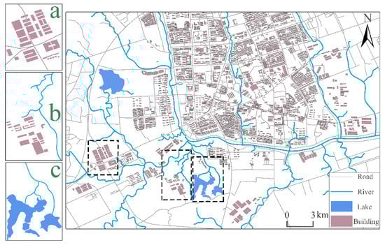
Figure 1.
Map and the extracted micro scenes (a) (block composed of roads and buildings), (b) (an urban waterfront composed of buildings and rivers), and (c) (a river system formed by rivers and lakes).
In practical applications, micro scenes are the basis for hand-drawn scene navigation, fragment scene positioning, and criminal investigation analysis. Numerous studies have attempted to compare scenes based on geometric similarities [18,19]. However, the definition and representation of similarity are complex, and human expression and cognition relative to space are hierarchical [20,21,22]. Almost all of the existing geometric similarity theories, methods, and models are imperfect. The central question of micro scene comparisons is how to associate objects and relationships in one scene to corresponding objects and relationships in another scene. Therefore, it is important to identify what factors should guide the correspondence amongst them.
Our purpose in this study was to research the preservation of micro scenes’ geometric similarity in generalization, and to apply the geometric similarity to evaluate the quality of cartography. Therefore, we chose the three basic geometric characteristics of shape, direction, and position [23], upon which geometric similarity or matching is often based [24]. Complex structures exist in the spatial objects of micro scenes. In the process of calculating similarity, it is necessary to comprehensively calculate the overall shape similarity and the direction similarity, and the position similarity of the objects should also be considered.
Thus, we constructed a method for measuring the geometric similarities of micro scene generalizations, which considers the transformations in shape, direction, and position. The improvements mainly include: (1) a proposed method for accounting the relationships amongst the geometrical shape, direction, and a position of a micro scene during cartographic generalization; and (2) a method that is able to quantitatively evaluate the preservation of geometric features between original micro scenes and their generalized counterparts.
2. Methodology
A micro scene contains line groups and polygon groups; shape transformation, direction transformation, and position transformation should be considered in the similarity calculation of micro scenes (Figure 2). In this study, we constructed a method of evaluating the geometric similarity of micro scenes based on hybrid feature description, a direction Voronoi diagram, and a position graph. Shape similarity was calculated by combining the Included Angle Chain and the Hausdorff distance; the directional Voronoi diagram was used to calculate the direction similarity; the Delaunay triangulation network was constructed to calculate the position similarity.
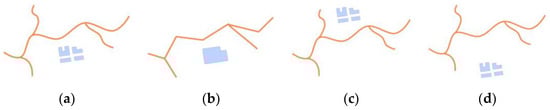
Figure 2.
Factors affecting micro scenes in similarity judgements: (a) original object group; (b) shape transformation; (c) direction transformation; (d) position transformation.
2.1. Shape Similarity
The extraction algorithm for shape features needs to convert the original node sequence into a feature description sequence [25]; the more detailed the descriptions of the morphological features, the more accurate the similarity calculation results [26]. In addition, the algorithm should include the extraction of global and local features [27]. The former involves the use statistical methods to extract global features, such as area, perimeter, circumscribed rectangle, and Hausdorff distance, from geometric figures; the latter describes the local structure of the graph based on curvature [28], key points [29], concave-convex morphology [30], Hough variation [31], etc.
To ensure the accuracy of calculation and to describe complex shapes, this paper proposes a hybrid features description method that combines Included Angle Chain and Hausdorff distance.
We treated polygons as closed line features to calculate the shape similarity of the micro scenes, and the direction Voronoi graph and position graph were constructed. The micro scene similarities were calculated through shape similarity, direction similarity and position similarity.
2.1.1. Shape Feature Extraction by Included Angle Chain
Included Angle Chain [32] is one of the main methods used for the shape similarity analyses of linear features. Its basic idea is as follows:
Two curves are fitted with n line segments of equal length, and the angles between the adjacent line segments are used to form their respective angle sequences (i.e., Included Angle Chain). Then, the similarities between the linear features are measured by calculating the differences in the angle sequences.
The generation process of the isometric polyline is as follows: First, the Minimum Bounding Rectangle (MBR) of the curve is determined, taking the longer side as L1, and then a circle with radius L1/n and the node as the center is drawn. The intersection of the circle and the curve serves as the end of the line segment, and this point is also the center of the second circle (if there are multiple intersections, we select the point closest to the starting point). Then, the above steps are repeated in sequence to obtain the nth intersection In; if the end of the curve is not reached, the remaining curve is regarded as a complete curve, and the above operation is repeated. Finally, within range of error δ, the length of the isometric polyline is obtained after m cycles. The length calculation formula is shown in Equation (1):
2.1.2. Shape Feature Extraction by Hausdorff Distance
The Hausdorff distance reflects the proximity of positions between curves, and similarity is calculated by measuring the distance between discrete point sets. The basic idea is as follows:
Assuming point sets A = {a1, a2, … am} and, B = {b1, b2, … bn} the calculation using the Hausdorff distance calculation formula is as shown in Equation (2):
where h (A, B) and h (B, A) are one-way Hausdorff distances, representing the maximum of the minimum distances between all points in a set of points and another set of points. The details are shown as Equation (3).
2.1.3. Shape Feature Extraction by Hausdorff Distance and Included Angle Chain
The Included Angle Chain is suitable for the calculation of local similarity, but the global features of a curve cannot be described by only the Euclidean distance of the angle chain [33]. The Hausdorff distance is often used as a method of measuring geometric similarity, but its disadvantage is that only the maximum offset value is considered; the detailed features of the curve are not reflected [34].
Thus, this paper proposes a shape similarity calculation method that combines the Included Angle Chain and Hausdorff distance under a curvature constraint. The method is mainly divided into the following three steps:
Step 1: The process of using the Included Angle Chain to determine the equal-length polyline is time consuming, and the curve may not be equally divided into n at the same time. In view of this, the process is transformed in the process of dividing a curve into equal segments, and the curvature is used as the basis of the equal division of the curve.
Taking Figure 3 as an example, the black lines are curves P and Q, which are to be compared, and the number of nodes is m and n; P = ((px,1, py,1), (px,2, py,2),…, (px,m, py,m)), Q = ((qx,1, qy,1), (qx,2, qy,2),…, (qx,m, qy,m)). The red line and the green line are the fitted lines, which are composed of a sequence of equal points, and angle sequences (α1, α2 … α9) and (β1, β2 … β9) are obtained.
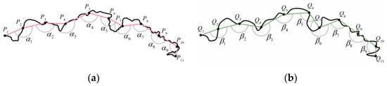
Figure 3.
Curve shape feature extraction: (a) curve P; and (b) curve Q.
To further extract the morphological features of a curve, the number of equally divided segments needs to be increased. Since the first and second derivatives at the node can be approximated by numerical differentiation, the curvature at the node (ax,i, ay,i) is as shown in Equation (4).
Here, and are the first partial derivatives at the node, respectively; and are the second partial derivatives, respectively.
Given a curvature threshold ζ, the mean value of the absolute curvature of each segment is sorted. When the sorted value is less than ζ, the equal division of the linear feature is stopped.
Step 2: The angle sequence and the corresponding length sequence are synthesized to obtain feature sets: M = {(p1, α1), (p2, α2) … (p9, α9)} and N = {(q1, β1), (q2, β2) … (q9, β9)}. Coordinate origin O is taken as the pole, the counterclockwise direction is treated as the positive direction, the length is treated as the polar diameter, and the angle is treated as the polar angle. Then, Equation (5) is used to scatter the points sequence, and the polar coordinate systems (pi, αi) and (qi, βi) are constructed (Figure 4). Finally, according to x = ρcosθ, y = ρsinθ, the polar coordinates are converted into rectangular coordinates, and the feature point sequences of the curves are converted into description sequences of geometric features.
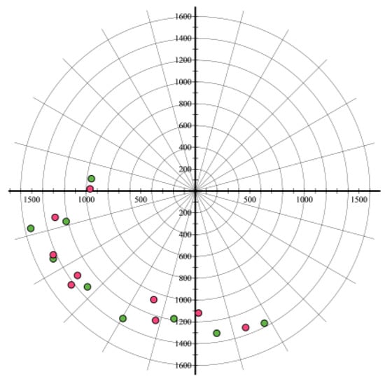
Figure 4.
Feature point sets of curve P and curve Q.
Step 3: The median Hausdorff distance of the point groups is calculated, and the similarity between the two curves can be obtained according to:
where HM,P(P, Q) and HM,Q(P, Q) are the median Hausdorff distance, and is the similarity between P and Q.
2.1.4. Double Lines Shape Similarity Calculation
The method of a constructing skeleton line can describe the shape features of a simple double line to some extent [35]. In Figure 5, the black lines are the curves to be compared and the red lines are the extracted skeleton lines. Shape recognition and element matching can be performed by comparing the geometric features between the skeleton lines.
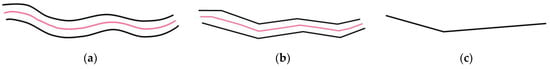
Figure 5.
Shape feature extraction of constructed skeleton lines: (a) original data; (b) the first generalization; (c) the second generalization.
However, this method has certain limitations, such as the four types of double-lines (Figure 6a–d) being converted into straight lines after generalization (Figure 6e). If we use the linear features of generalization or skeleton lines to calculate the geometric similarity, the calculated result will be too large, which is inconsistent with visual perception.
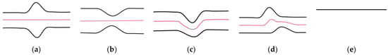
Figure 6.
Several types of double lines: (a) convex symmetry; (b) concave symmetry; (c) curvature difference; (d) misplaced; (e) final generalized result.
The above-mentioned situations mostly occur in fine-grained line groups, such as curved sections and transition sections of a river system, multilane roads, and complex interchanges in road networks. Hence, this method is unable to describe complex shapes, and an effective shape extraction approach should consider the geometric features of both sides of double lines.
We expanded the calculation method of the single line shape similarity that combines the Included Angle Chain and Hausdorff distance under a curvature constraint. We take Figure 7a,b as examples for the similarity calculation of a double line.
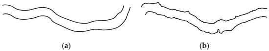
Figure 7.
Curves to be compared: (a) curve A’s; and (b) curve B’s features’ description sequence.
Firstly, dividing the double line into an upper curve and a lower curve , the curvature constraint thresholds of the curves are and , respectively. Then, curves and are initially segmented, the segment curvature is calculated, and the feature description set of the upper curve and the lower curve is obtained. By integrating them under the same coordinate system (Figure 8a,b), the geometric similarity between curve A and curve B is calculated using Equation (7).
where represents the upper and lower curves, and is the similarity between A and B.
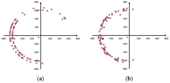
Figure 8.
Extraction of curves’ shape feature point: feature description sequence of (a) curve A and (b) curve B.
2.1.5. Micro Scenes’ Shape Similarity
Humans’ expression and cognition of space are hierarchical, and the multilevel expression of space aligns with the human cognitive perception of space [36,37]. The morphology similarity calculation is based on multilevel grids, where the larger the grid size, the fewer the number of grids; the details of spatial objects are generalized, which can only reflect the global distribution of features. The smaller the grid, the more detailed the description of objects, and the more detailed the extraction of local structural features [38].
Initial grids are constructed and the regions are divided into several levels according to hierarchical control index N. The calculation of N is shown in Equation (8), using the maximum density, minimum density, and the visual discrimination coefficient to estimate the number of levels [39,40].
Here, Dmax is the maximum density, Dmin is the minimum density, and q is the visual discrimination coefficient of the map load.
The geometric similarity of each grid is calculated according to:
where and are the median Hausdorff distance, and SimGrid is the shape similarity between GridA and GridB.
Finally, the shape similarity calculation formula is obtained according to the percentage of the length (Equation (10)):
where w1, w2 and wn are the percentages of each type of grid in the total length, and Simshape is the shape similarity.
2.2. Direction Similarity
Direction relationships between object groups play an important role in spatial computation and spatial recognition. A number of models for the description and computation of direction relations have been proposed, including the cone-based model [41], the 2-D projection model [42], the direction-relation matrix model [43], the statistical weighting orientation [44], and the Voronoi-based model [45].
2.2.1. Direction Voronoi Graph Model
The direction Voronoi graph model considers all sides of the directional relationships between two targets, and uses a set of multiple directions to describe the directional relationships.
To simplify the discussion, the two object groups in Figure 9a are used as an example. The specific calculation process is divided into the following five steps:
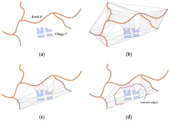
Figure 9.
Procedures for computing direction relationships between two object groups: (a) the object groups; (b) triangulation of the object groups; (c) proximal sections of the object groups; and (d) direction Voronoi diagram.
- Construct a point set of the two object groups.
- Generate the Voronoi diagram. If the three vertices of a triangle belong to the same object group, it is called the first type of triangle; otherwise, it is called the second type of triangle (Figure 9b).
- Delete the first type of triangles, and the remaining triangles form a visible triangulation network (Figure 9c). The area covered by the triangulation network is the visible area between the targets.
- Connect the midpoints of the triangle waists to generate the Voronoi diagram of the direction (Figure 9d).
- Calculate the azimuth angle of the normal of each Voronoi side, and use the eight-direction system to classify the azimuths within the same direction into one category. Then, calculate the percentage of the length of the Voronoi side in each main direction. As such, the precise directional relationship between group targets can be obtained.
2.2.2. Micro Scenes’ Direction Similarity
The direction Voronoi diagram model uses the 8-direction system to calculate the percentage of the Voronoi edge in each main direction to obtain the direction relationship, and it cannot be directly applied to the calculation of direction similarity [46]. For example, for the case shown in Figure 10, Table 1 provides the calculation result of the direction relationship. The result is semi-qualitative, and the percentages in each direction cannot be directly applied to similarity calculations.
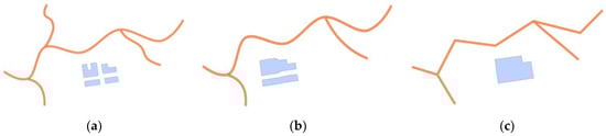
Figure 10.
Object group generalization: (a) original data, (b) the first generalization, and (c) the second generalization.

Table 1.
Computation results of the direction relationship.
As such, we constructed a direction similarity measurement method that combines a direction Voronoi diagram and Hausdorff distance. This method quantifies the overall distribution characteristics of the direction Voronoi diagram, and calculates the directional similarity through the Hausdorff distance.
Firstly, the equipartition spacing of lines and polygons is determined using Equation (11), and the direction Voronoi diagram is constructed (Figure 11).
where Int[] is a function that returns the integer part, and MapScale (A) is the scale denominator of data A. MapScale (A)/1000 indicates the actual length of the graph corresponding to 1 mm, 1⁄10 represents the proportion that can be recognized by human eyes at a distance of 1 mm on the drawing, and ε represents the distance tolerance coefficient.
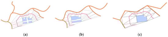
Figure 11.
Construction of direction Voronoi diagram: (a–c) the directional Voronoi diagrams constructed using the three scales of micro scenes.
Subsequently, the ratio of the area of the triangle in each direction to the total area is calculated so that it can be used as the X coordinate. The ratio of the length of each line segment to the total length is used as the Y coordinate. The size of the direction angle is used as the offset value of the Z axis. Thereby, a three-dimensional feature point set describing the direction relationship is obtained (Figure 12).
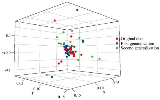
Figure 12.
Feature point set of the direction relationship.
Then, the directional similarity between the micro scenes is calculated by the Hausdorff distance of the feature point set. The calculation formula is as follows:
where and are the median Hausdorff distance, and Simdirection is the direction similarity between S1 and S2.
2.3. Position Similarity
The position similarity calculation of the micro scenes needs to consider the positional relationship between lines and lines, lines and polygons, and polygons and polygons. In this paper, the position similarity between the elements is obtained through the construction of the position graph.
2.3.1. Position Graph
Generally, the position similarity is obtained by calculating the center distance between objects, where position graphs and Delaunay triangulation are commonly used methods [47,48]. Micro scenes contain lines and polygons, and the positional relationship between features needs to be described separately. Delaunay triangulation has been widely used in the description of spatial relations and it meets the above requirements. We selected Figure 10a as an example; three types of triangles describing position relationships were obtained through the construction of Delaunay triangulation (Figure 13).
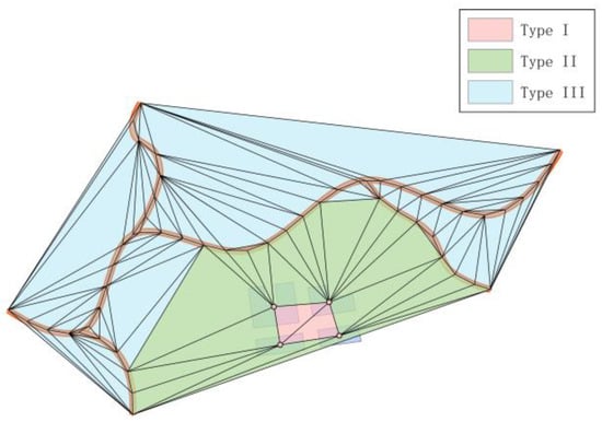
Figure 13.
Construction of position graph.
The first type of triangulation describes the position relationships between polygons, the second triangulation describes the position relationships between lines and polygons, and the third triangulation describes the position relationships between lines.
2.3.2. Micro Scenes Position Similarity
It is necessary to calculate the similarity of these triangles separately, and the similarity of any two triangles can be calculated according to the fuzzy similarity method. The specific process is as follows:
First, a pair of similar triangles is taken and marked as ΔABC and ΔA’B’C’, and the corresponding vertex angle degrees are denoted as θa and θ’a. The similarity of the corresponding internal angles of the triangle is denoted as Sima, Simb, and Simc, and the angle similarity equation is:
Then, the similarity of the other two pairs of vertices is obtained using Equation (13), and the similarity of this pair of triangles is:
The similarity of all triangles in the Delaunay triangulation of the two images is calculated using Equations (13) and (14) to construct the following similarity M × N matrix:
The mean value is:
Subsequently, the position similarity of each type of triangulation is:
Finally, the position similarity calculation formula is obtained according to the percentage of the area:
where w1, w2, and w3 are the percentages of each type of triangulation in the total area, and Simposition is the position similarity.
2.4. Geometric Similarity Measurements of Micro Scenes
At present, the overall similarity is mainly determined through the weight calculation of each similarity index, and the similarity calculation formula is obtained by combining the similarity evaluation factors. However, due to the complex structure of the micro scenes, the analytic hierarchy process (AHP) and entropy methods have certain limitations. These methods may be suitable for specific areas, but they are not capable of describing a wider range of situations. For example, the weight value of river + islands obtained through AHP is not applicable to roads + buildings.
Referring to recent research [31,49], we took the geometric mean of the direction similarity, position similarity, and shape similarity as the value of the global similarity (Equation (19)); we found the calculation results were more stable and more in line with the actual situations by tests, indicating the geometric mean is suitable for the micro scene similarity calculation.
Here, Simshape is the shape similarity calculated by Equation (10), Simdirection is the direction similarity calculated by Equation (12), Simposition is the position similarity calculated by Equation (18), and SIM is the overall similarity.
3. Experiments and Analysis
To fully test the performance of the presented approach, a Fourier shape descriptor was implemented to conduct a contrast experiment. In the first experiment, we applied the proposed method to calculate the similarities of micro scene. In the second experiment, we applied similarity to evaluate the quality of micro scene generalization.
3.1. Study Area and Data
The experiments were based on a preprocessed GF-2 remote sensing image (Figure 14); the study area was Lanzhou, China. The image acquisition time was 6 December 2016, and the coordinate system was WGS-84.
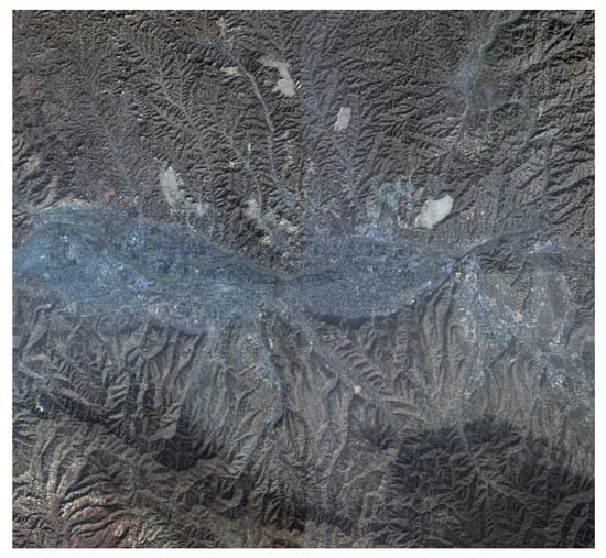
Figure 14.
The original remote sensing image.
3.2. Similarity Measurement for Micro Scene Generalization
The purpose of this part of the study was to verify the usability of the experimental methods in the detection of changes in the shape, direction, and position of micro scenes. We extracted five micro scenes (Figure 15a–e) from the remote sensing image: Figure 15a,b depicts the complex river section formed by islands and rivers, Figure 15c is the river system composed of rivers and lakes, Figure 15d depicts the urban waterfront, and Figure 15e shows the block composed of roads and buildings. Four basic operations of displacement, simplification, merging, and deletion in cartographic generalization were carried out sequentially. Similarities between each micro scene were computed, and the experimental results are shown in Figure 16.
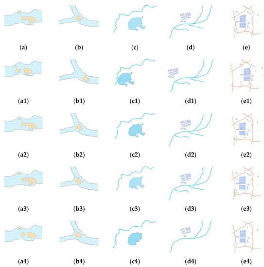
Figure 15.
Original data and generalization data: (a–e) the original data; (a1–e1) the data after the displacement operation; (a2–e2) the data after the simplify operation; (a3–e3) the data after the merge operation; and (a4–e4) the data after the delete operation.
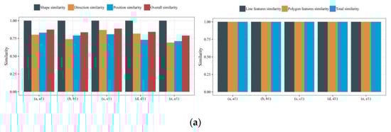
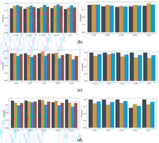
Figure 16.
The similarity of the original data and generalization data calculated by the proposed method and the Fourier shape descriptor: (a) displacement operation; (b) simplify operation; (c) merge operation; (d) delete operation.
Figure 16a shows that the shape similarities of the five micro scenes obtained by the proposed method are all one, and the directional and positional similarities change considerably. Taking the set (a, a1) as an example, the positional similarities of the first and third types of triangulation are both one, indicating that the relative position of island to island and river bank to river bank has not changed; the similarity of the second type of triangulation is 0.740, indicating that the relative position between the islands and the river banks changed. The similarities calculated by the Fourier shape descriptor are all one, which is inconsistent with the actual situation. This is because Fourier calculates the similarities of line features and polygon features separately, ignoring the direction and position relationship between the elements of the micro scenes.
Figure 16b provides the calculation result of the similarity between the original data and the simplified data. The shapes of the five micro scenes calculated by the proposed method changed markedly, but the changes in position and direction are small, which is consistent with the actual situation. The Fourier calculation results only showed that the similarities of the line group and polygon group reduced, and the specific operations could not be deduced from the calculation results.
According to the calculation results of the proposed method, we found that the position similarity of the five micro scenes was relatively low, and the direction and shape similarities were high (Figure 16c). The Fourier calculation results showed that the similarity of line features did not change, but the similarity of polygon features changed considerably. The above results showed that the two methods are complementary under the merge operation.
From the calculation results of the proposed method, we found that the position similarity changes greatly, and the changes in shape and direction similarities were small (Figure 16d), which is in line with the characteristics of the deletion operation. Fourier detected that the object of the deletion operation was mainly polygon features, but in the (d, d1) set, we deleted both line features and polygon features, and the calculation results did not show the type of cartography operation.
In conclusion, Fourier divides micro scenes into independent line features and polygon features to calculate similarity, which breaks the overall connection between the objects in the micro scenes and cannot express the direction and position changes in the process of generalization. The proposed method compensates for the above shortcomings, and the similarity calculation results are more in line with the actual situation.
3.3. Quality Assessment of Micro Scene Generalization
The main purpose of this part of the study was to verify the effectiveness of applying geometric similarity to assessing the quality of micro scene generalization. We chose Figure 17a–e as the original data, and small-scale maps were generated on this basis. The similarities between each micro scene were computed, and the experimental results are shown in Table 2 and Table 3.
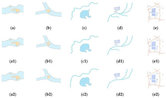
Figure 17.
Generalization results of micro scenes: (a–e) original data; (a1–e1) the results of the first generalization; (a2–e2) the results of the second generalization.
Table 2.
Calculation results produced by the method proposed in this paper.
Table 3.
Calculation results of Fourier shape descriptor.
From the calculation results in Table 2 and Table 3, we found that as the degree of generalization increased, the similarity between the two methods gradually decreased. However, the Fourier shape descriptor breaks the overall connection between the objects in the micro scenes and cannot express the direction and position changes in the process of generalization. Only the similarity of a single feature can be described through the Fourier shape descriptor; it cannot be directly applied to the quality evaluation of micro scene generalization. However, the proposed method compensates for this deficiency.
In the map generalization process, we used the selection and merging methods. Some islands, buildings, and lakes were discarded, and smaller units were merged, which caused (1) the similarity of the second and third types of triangular nets to be reduced, and (2) the direction difference between composite features to increase and the similarity between micro scenes to decrease. In addition, the simplification method reduces the details, and the shape similarity is decreased. The details of the similarity changes between micro scenes are as follows:
In the river + islands micro scene, such as in Figure 17a–a2,b–b2, the simplification operation of the river caused the main shape to change, and the changes in direction similarity and position similarity mainly occurred due to the deletion of islands. In Figure 17a–a2, the shape similarities dropped from 0.923 to 0.818; the position similarities of the first type changed from 0.847 to 0.759, and the second changed from 0.791 to 0.656. These calculation results are consistent with the actual situation.
In the river +lakes micro scene, as shown in Figure 17c–c2, due to the generalization operation between river and lakes, the directional similarity decreased, and the changes in position similarity occurred due to the merge operation. In Figure 17c–c2, the directional similarity dropped from 0.819 to 0.730, and the positional similarities of the first type dropped from 0.864 to 0.679. The calculation results detected the changes in the position and direction before and after generalization.
In the rivers + buildings micro scene, such as in Figure 17d–d2, the change in direction similarity was small, and the change was mainly due to the merge operation. For Figure 17d–d2, the change rate of directional similarity was 5.05%, and the positional similarities dropped from 0.785 to 0.703.
In the roads + buildings micro scene, such as in Figure 17e–e2, the change in directional similarity was small, and the change was due to the merge operation. For Figure 17e–e2, the change rate in direction similarity was 5.63%, and the change rate of position similarity was 13.26%; the results are consistent with the actual situation.
The proposed method comprehensively considers the overall distribution relationships between features in micro scenes, and measures the changes in shape, direction, and position. Overall, the calculation results are more consistent with the actual situation, and the changes in geometric similarity before and after generalization can be quantitatively evaluated.
4. Conclusions
In this study, we examined the geometric similarity of micro scenes from the perspective of generalization. The geometric similarity changes in the micro scene were described from three aspects: shape similarity, direction similarity and position similarity. This study’s findings contribute to existing research on cartographic generalization by analyzing the geometric features and the generalization process.
The findings illustrated that the three factors can quantitatively describe the geometric similarity changes in micro scene generalization. In the river + islands micro scene, the simplification operation caused the shape similarities to decrease from 0.923 to 0.818, and the delete and merge operations caused the position similarity to change from 0.769 to 0.692. In the river +lakes micro scene, the changes in position similarity occurred due to the merge operation, and the directional similarity dropped from 0.819 to 0.730. In the rivers + buildings and roads + buildings micro scenes, the change rates of directional similarity were 5.05% and 5.63%, respectively; the changes mainly came from the deletion and simplification operations.
In general, the geometric similarities of micro scenes can be comprehensively calculated, even if they contain different types of geographic features. The proposed method effectively detects the changes in shape, direction, and position during generalization. In addition, it is able to quantitatively evaluate the preservation of geometric features between original micro scenes and their generalized counterparts; the calculation results were more in line with the actual situation.
However, several issues should be investigated further. The proposed approach could be improved further by considering the constraints of spatial relationships, such as topological constraints, and the method should be extended to the similarity calculation of multiscale and multi-morphological micro scenes. In addition, automatic micro scene extraction and segmentation methods need to be further studied.
Author Contributions
Z.W. helped conceive and design the study; F.Y. carried out the method and wrote the manuscript; H.Y. and X.L. offered significant contribution to result evaluation. All authors have read and agreed to the published version of the manuscript.
Funding
This research was funded by National Natural Science Foundation of China (No. 41930101, 41861060, 42161066, and 42174003), Local Science and Technology Development Fund Projects under the Guidance of Central Government, Gansu Province Natural Sciences Fund (No. 637020), and LZJTU EP (No. 201806).
Institutional Review Board Statement
Not applicable.
Informed Consent Statement
Not applicable.
Data Availability Statement
Not applicable.
Acknowledgments
We sincerely appreciate the Editor’s encouragement and the anonymous reviewer’s valuable support.
Conflicts of Interest
The authors declare that they have no conflict of interest.
References
- Ali, A.R.; Chehreghan, A.; Karimi, A. Assessing the efficiency of shape-based functions and descriptors in multi-scale matching of linear objects. Geocarto Int. 2018, 33, 879–892. [Google Scholar]
- Kim, J.; Yu, K.; Bang, Y. A multi-criteria decision-making approach for geometric matching of areal objects. Trans. GIS 2018, 22, 269–287. [Google Scholar] [CrossRef]
- Fan, H.; Yang, B.; Zipf, A. A polygon-based approach for matching OpenStreetMap road networks with regional transit authority data. Int. J. Geogr. Inf. Sci. 2016, 30, 748–764. [Google Scholar] [CrossRef]
- Mackaness, W.A.; Ruas, A. Evaluation in the map generalisation process. In Generalisation of Geographic Information; Elsevier Science BV: Amsterdam, The Netherlands, 2007; pp. 89–111. [Google Scholar]
- Yu, W. Quality assessment in point feature generalization with pattern preserved. Trans. GIS 2018, 22, 872–888. [Google Scholar] [CrossRef]
- Tang, L.; Li, Q.; Yang, B. Shape similarity measuring for multi resolution transmission of spatial datasets over the Internet. Acta Geod. Et Cartogr. Sin. 2009, 38, 336–340. [Google Scholar]
- Tian, R.; Li, S.; Yang, G. Traffic Flow Data Preprocessing Method Based on Spatio-temporal Similarity. In Proceedings of the 2017 International Conference Advanced Engineering and Technology Research (AETR 2017), Xi’an, China, 29–31 December 2017; Atlantis Press: Paris, France, 2018; pp. 128–131. [Google Scholar]
- Zhou, X.; Wang, H.; Wu, Z. An incremental updating method for land cover database using refined 2-dimensional intersection type. Acta Geod. Et Cartogr. Sin. 2017, 46, 114–122. [Google Scholar]
- Kim, J.Y.; Yu, K.Y. Automatic detection of the updating object by areal feature matching based on shape similarity. J. Korean Soc. Surv. Geod. Photogramm. Cartogr. 2012, 30, 59–65. [Google Scholar] [CrossRef][Green Version]
- Zhang, X.; Stoter, J.; Ai, T. Automated evaluation of building alignments in generalized maps. Int. J. Geogr. Inf. Sci. 2013, 27, 1550–1571. [Google Scholar] [CrossRef]
- Stoter, J.; Burghardt, D.; Duchêne, C. Methodology for evaluating automated map generalization in commercial software. Comput. Environ. Urban Syst. 2009, 33, 311–324. [Google Scholar] [CrossRef]
- Harrie, L.; Stigmar, H.; Djordjevic, M. Analytical estimation of map readability. ISPRS Int. J. Geo-Inf. 2015, 4, 418–446. [Google Scholar] [CrossRef]
- Cuenin, R. Cartographie générale: Tome 1: Notions générales et principes d’élaboration; Eyrolles: Paris, France, 1972. [Google Scholar]
- Shen, Y.; Ai, T.; Wang, L. A new approach to simplifying polygonal and linear features using superpixel segmentation. Int. J. Geogr. Inf. Sci. 2018, 32, 2023–2054. [Google Scholar] [CrossRef]
- Chehreghan, A.; Ali Abbaspour, R. An assessment of spatial similarity degree between polylines on multi-scale, multi-source maps. Geocarto Int. 2017, 32, 471–487. [Google Scholar] [CrossRef]
- Zhang, W.B.; Ge, Y.; Leung, Y.; Zhou, Y. A georeferenced graph model for geospatial data matching by optimising measures of similarity across multiple scales. Int. J. Geogr. Inf. Sci. 2020, 34, 1–17. [Google Scholar] [CrossRef]
- Yong, X.; Zhong, X.; Chen, Z.; Liang, W. Shape similarity measurement model for holed polygons based on position graphs and Fourier descriptors. Int. J. Geogr. Inf. Sci. 2016, 31, 253–279. [Google Scholar]
- Stefanidis, A.; Agouris, P.; Georgiadis, C. Scale-and orientation-invariant scene similarity metrics for image queries. Int. J. Geogr. Inf. Sci. 2002, 16, 749–772. [Google Scholar] [CrossRef][Green Version]
- Nedas, K.A.; Egenhofer, M.J. Spatial-scene similarity queries. Trans. GIS 2008, 12, 661–681. [Google Scholar] [CrossRef]
- Gavrila, D.M. A Bayesian, Exemplar-Based approach to hierarchical shape matching. IEEE Trans. Pattern Anal. Mach. Intell. 2007, 29, 1408–1421. [Google Scholar] [CrossRef]
- Latecki, L.J.; Lakamper, R. Shape similarity measure based on correspondence of visual parts. IEEE Trans. Pattern Anal. Mach. Intell. 2000, 22, 1185–1190. [Google Scholar] [CrossRef]
- Zhou, M.; Hu, W.; Ai, T. Multi-level thematic map visualization using the Treemap hierarchical representation model. J. Geovisualization Spat. Anal. 2020, 4, 1–11. [Google Scholar] [CrossRef]
- Acton, C.; Bachman, N.; Semenov, B. A look towards the future in the handling of space science mission geometry. Planet. Space Sci. 2018, 150, 9–12. [Google Scholar] [CrossRef]
- Yan, H.; Chu, Y. On the fundamental issues of spatial similarity relations in multi-scale maps. Geogrphy Geo-Inf. Sci. 2009, 25, 42–44. [Google Scholar]
- Sebastian, T.B.; Kimia, B.B. Curves vs skeletons in object recognition. Signal Process. 2005, 85, 247–263. [Google Scholar] [CrossRef]
- Wang, S.; Ji, H.; Li, P.; Li, H.; Zhan, Y. Growth diffusion-limited aggregation for basin fractal river network evolution model. AIP Adv. 2020, 10, 075317. [Google Scholar] [CrossRef]
- Zeng, J.; Zhan, L.; Fu, X. Straight line matching method based on line pairs and feature points. IET Comput. Vis. 2016, 10, 459–468. [Google Scholar] [CrossRef]
- Federer, H. Curvature measures. Trans. Am. Math. Soc. 1959, 93, 418–491. [Google Scholar] [CrossRef]
- An, X.; Liu, P.; Yang, Y.; Hou, S. A geometric similarity measurement method and applications to linear feature. Geomat. Inf. Sci. Wuhan Univ. 2015, 40, 1225–1229. [Google Scholar]
- Li, Z.; Zhai, J.; Fang, W. Shape similarity assessment method for coastline generalization. ISPRS Int. J. Geo-Inf. 2018, 7, 283. [Google Scholar] [CrossRef]
- Xu, Y.; Xie, Z.; Chen, Z.; Xie, M. Measuring the similarity between multi-polygons using convex hulls and position graphs. Int. J. Geogr. Inf. Sci. 2021, 35, 847–868. [Google Scholar] [CrossRef]
- Zhao, Y.; Chen, Y.Q. Included angle chain: A method for curve representation. J. Softw. 2004, 15, 300–307. [Google Scholar]
- Ohbuchi, R.; Minamitani, T.; Takei, T. Shape-similarity search of 3d models by using enhanced shape functions. Int. J. Comput. Appl. Technol. 2005, 23, 70–85. [Google Scholar] [CrossRef]
- Min, T.; Lee, M.; Kim, Y.J. Interactive Hausdorff distance computation for general polygonal models. ACM Trans. Graph. (TOG) 2009, 28, 1–9. [Google Scholar] [CrossRef]
- Yang, B.; Zhang, Y. Pattern-mining approach for conflating crowdsourcing road networks with POIs. Int. J. Geogr. Inf. Sci. 2015, 29, 786–805. [Google Scholar] [CrossRef]
- Brodeur, J.; Bédard., Y.; Edwards, G.; Moulin, B. Revisiting the concept of geospatial data interoperability within the scope of human communication processes. Trans. GIS 2003, 7, 243–265. [Google Scholar] [CrossRef]
- Jiang, X.; Center, C.G. The multi-scale expression design for web map based on map visual perception. Geomat. Spat. Inf. Technol. 2014, 37, 43–45. [Google Scholar]
- Shoman, W.; Alganci, U.; Demirel, H. A comparative analysis of gridding systems for point-based land cover/use analysis. Geocarto Int. 2019, 34, 867–886. [Google Scholar] [CrossRef]
- Guo, D. Geospatial Analysis Based on Similar Spatial Scenes; Science Press: Beijing, China, 2016; pp. 57–83. [Google Scholar]
- Wu, H. Basic Model and Algorithm of GIS and Map Information Generalization; Wuhan University Press: Wuhan, China, 2012; pp. 115–130. [Google Scholar]
- Peuquet, D.; Zhan, C. An algorithm to determine the directional relation between arbitrarily-shaped polygons in the plane. Pattern Recognit. 1987, 20, 65–74. [Google Scholar] [CrossRef]
- Frank, A.U. Qualitative spatial reasoning about distances and directions in geographic space. J. Vis. Lang. Comput. 1992, 3, 343–371. [Google Scholar] [CrossRef]
- Goyal, R.K. Similarity Assessment for Cardinal Directions between Extended Spatial Objects; The University of Maine: Orono, ME, USA, 2000. [Google Scholar]
- Duchêne, C.; Bard, S.; Barillot, X.; Ruas, A.; Trevisan, J.; Holzapfel, F. Quantitative and Qualitative Description of Building Orientation. In Proceedings of the Fifth Workshop on Progress in Automated Map Generalisation, ICA, Commission on Map Generalisation, Paris, France, 28–30 April 2003. [Google Scholar]
- Yan, H.; Wang, Z.; Li, J. An approach to computing direction relations between separated object groups. Geosci. Model Dev. 2013, 6, 1591–1599. [Google Scholar] [CrossRef]
- Chen, Z.; Gong, X.; Wu, L.; An, X. A quantitative calculation method of composite spatial direction similarity concerning scale differences. Acta Geod. Et Cartogr. Sin. 2016, 45, 362–371. [Google Scholar]
- Ai, T.; Shu, K.; Min, Y.; Li, J. Envelope generation and simplification of polylines using Delaunay triangulation. Int. J. Geogr. Inf. Sci. 2017, 31, 297–319. [Google Scholar] [CrossRef]
- Sundaram, V.M.; Paneer, P. Discovering Co-Location patterns from spatial domain using a Delaunay approach. Procedia Eng. 2012, 38, 2832–2845. [Google Scholar] [CrossRef]
- Touya, G. Multi-criteria geographic analysis for automated cartographic generalization. Cartogr. J. 2021, 1–17. [Google Scholar] [CrossRef]
Publisher’s Note: MDPI stays neutral with regard to jurisdictional claims in published maps and institutional affiliations. |
© 2022 by the authors. Licensee MDPI, Basel, Switzerland. This article is an open access article distributed under the terms and conditions of the Creative Commons Attribution (CC BY) license (https://creativecommons.org/licenses/by/4.0/).