Superpixel Image Classification with Graph Convolutional Neural Networks Based on Learnable Positional Embedding

Abstract

Graph convolutional neural networks (GCNNs) have been successfully applied to a wide range of problems, including low-dimensional Euclidean structural domains representing images, videos, and speech and high-dimensional non-Euclidean domains, such as social networks and chemical molecular structures. However, in computer vision, the existing GCNNs are not provided with positional information to distinguish between graphs of new structures; therefore, the performance of the image classification domain represented by arbitrary graphs is significantly poor. In this work, we introduce how to initialize the positional information through a random walk algorithm and continuously learn the additional position-embedded information of various graph structures represented over the superpixel images we choose for efficiency. We call this method the graph convolutional network with learnable positional embedding applied on images (IMGCN-LPE). We apply IMGCN-LPE to three graph convolutional models (the Chebyshev graph convolutional network, graph convolutional network, and graph attention network) to validate performance on various benchmark image datasets. As a result, although not as impressive as convolutional neural networks, the proposed method outperforms various other conventional convolutional methods and demonstrates its effectiveness among the same tasks in the field of GCNNs.

1. Introduction

Convolutional neural networks (CNNs) have exhibited the best performance in many machine learning tasks, especially image processing [1,2,3]. However, the CNN structure has a rectangular-based grid data type, and the same input dimensions must be provided. Therefore, the application of CNNs to irregular atypical data (e.g., social networks and molecular structures) and 3D modeling, often encountered in real life, is limited. There are some studies that adapt CNNs on irregular domains but it therefore includes the design of classical convolutional layers as a particular case, in which the underlying graph is a grid [4]. Various problems that attempt to capture complex relationships or interdependencies between data can be expressed and analyzed more naturally in graphs.

Normally, goal of convolution operation is to summarize input data to a reduced form. Unfortunately, dot product to compute convolution is sensitive to the order, i.e., dot product is not permutation-invariant. So, convolution requires permutation-invariant operator that get the same result from a spatial region even if there is randomly shuffled pixels inside that region. CNNs can detect and recognize the object of image which translate to left or right by sharing same filter`s weights across all locations. However, it is difficult to define convolution on graphs. The main problem is that there is no well de-fined order of nodes in graphs because nodes are a set. So, unless we learn to order them, or come up with some heuristic that will result in a canonical order form graph to graph, applying a convolution to the graphs is meaningless.

Designed to be applied to graph data based on the CNN`s convolution, graph convolutional neural networks (GCNNs) use a permutation-invariant operator to aggregate information of nodes in any direction. The most popular choices are averaging [5] and summation [6] aggregator of all neighbors, so that GCNNs overcome the limitation of the ordering issue. Furthermore, GCNNs are not restricted to fixed dimensions of input and can flexibly treat different types of data in low-dimensional Euclidean (e.g., image [7,8,9,10,11,12,13,14,15,16,17,18,19], text [20], video [19]), and high-dimensional non-Euclidean domains (e.g., social network [21,22], and chemical molecules [23,24]). Based on the flexibility and extensionality of GCNNs, new approaches have recently been developed through graph representations of various data used in many deep learning fields.

In computer vision, some research has segmented original images into superpixel images, grouping perceptually meaningful pixels and preprocessing them into a graph to display the results in image classification [7,8,9,10], object detection [11,12,13,14], and semantic segmentation [15,16,17,18] based on GCNNs. Among these areas, we focus on the image classification task.

Generally, the superpixel image classification task requires procedures. First, a certain number of superpixels are generated from the original image using segmented algorithms [25,26,27]. Each superpixel region is defined as a node and connected to an edge through a region adjacency graph (RAG) [8,9,10]. These graph-represented images are input to spectrum-based [7,28,29] or spatial-based [5,30] GCNNs to learn the aggregated graph information during training and predict the class from it. However, even in the same class, the generated graph structures are arbitrary according to the different shapes of objects, and they are not sufficiently provided to the network to distinguish them. Thus, compared to the CNN, the results of the GCNNs are worse.

In this paper, we improve the power of GCNNs, according to Dwivedi et al. [31], by learning embedded positional information with structural information to create a more expressive graph representation in superpixel image classification. Furthermore, we use a specific loss function called ArcFace [32] that can supervise the learning process by increasing the angle difference among classes and decreasing it within classes based on the class-central weight vector and each feature vector to improve the result slightly.

This paper is organized as follows. Section 2 explains the superpixel segmentation algorithms and development of GCNNs with mathematical formulas and various methods from related work regarding superpixel image classification with GCNNs and graph positional embedding. Section 3 proposes the GCNNs with learnable positional embedding applied on images (IMGCN-LPE) and explains the ArcFace loss function in detail. Section 4 presents the comparative experiments and results with previous studies using various benchmark image datasets. Finally, the conclusion is drawn in Section 5.

2. Related Work

2.1. Superpixel Segmentation Algorithms

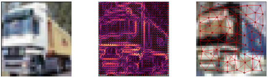
The superpixel method, frequently used in computer vision tasks, clusters pixels that share various common characteristics (color, location, etc.) in an image into one group. It is better than the original pixel, as the superpixel increases the computational efficiency by reducing the input size and number of learnable parameters. Moreover, it is much more practical for learning models by implicating perceptual information. There are many effective algorithms for segmenting images into superpixels, typically simple linear iterative clustering (SLIC) [25], Quickshift [26], and Felzenswalb [27]. Among the algorithms, SLIC is most commonly used in many studies because of its high stability and fast segmentation speed. We selected this algorithm for a fair comparison of the related work. Figure 1 presents a sample of the original images and the segmented pixel-based and SLIC-based graph images.

Figure 1. Sample of segmenting the original image into pixel-based and SLIC-based graph representation.

2.2. Advances in Graph Convolution definition

The application of graph representation in computer vision is usually conducted based on GCNNs. GCNNs emerged from the spectral-based graph convolution method, and many studies have been derived from this, as GCNNs produce good result. Therefore, as a step towards understanding GCNNs, we describe the advances in graph convolution definition, from the initial definition of graph convolution operation to the recent one, in this section.

Bruna et al. [28] initially defined the spectral graph convolutional method based on the convolution theorem in signal and image processing. In this paper, they defined a symmetric normalized Laplacian matrix (${ℒ}^{\mathrm{sym}}$) with a degree matrix ($\mathcal{D}$) and adjacency matrix ($\mathcal{A}$) from the structural graph information in Equation (1) and defined graph convolution using the eigenvector and eigenvalue from the eigendecomposition of $ℒ$^sym in Equation (2):

$${ℒ}^{\mathrm{sym}}=\mathsf{{\rm I}}-{\mathcal{D}}^{-\frac{1}{2}}\mathcal{A}{\mathcal{D}}^{-\frac{1}{2}}=U^T\Lambda U,$$

(1)

$$X^{l+1}=U(U^T{X}^l\odot U^T{W}_{spectral}^l).$$

(2)

where $\mathsf{{\rm I}}$ denotes the identity matrix, $U\in {ℝ}^{nxn}$ is the Fourier basis in which eigenvectors are treated with column vectors, $\Lambda \in {ℝ}^{nxn}$ is defined as a diagonal matrix of eigenvalues, $X^l\in {ℝ}^{nxF}$ is a feature vector in $l^{th}$ layer, $\odot$ represents the element-wise Hadamard product, and $W_{spectral}^l\in {ℝ}^{nxF}$ denotes the spectral convolutional filter.

However, due to the high dependence of graph size encoded by the eigenvector, it cannot be applied to the variable structure of the large-scale graph data. The computational cost is high because the complexity of the eigendecomposition related to the Fourier basis $U$ is $\mathcal{O}(n^2)$, where $n$ is the number of nodes in the graph.

To overcome this issue, Defferrard et al. [29] proposed the Chebyshev graph convolutional network (GCN) called ChebNet based on the Chebyshev polynomial in Equation (3), and the initial term is in Equation (4):

$$T_i(x)=2x{T}_{i-1}(x)-T_{i-2}(x),$$

(3)

$$T_0(x)=1, T_1(x)=x.$$

(4)

Based on the approximated filter by the K-order Chebyshev polynomial, the above graph convolutional method defines a localized filter by recursively aggregating only the information of nodes up to the $K^{th}$ distance from each node. Equation (5) defines an approximated filter $g_{\theta }$, and the convolutional operation for the input graph $G$ based on the filter is defined in Equation (6):

$$g_{\theta }\approx {\Sigma }_{k=0}^{K-1}{\theta }_k{T}_k( \tilde{\mathsf{\Lambda }}),$$

(5)

$$G\ast g_{\theta }\approx U({\Sigma }_{k=0}^{K-1}{\theta }_k{T}_k( \tilde{\mathsf{\Lambda }}))U^{T}G,$$

(6)

where $T_k(\tilde{\mathsf{\Lambda }})\in {ℝ}^{nxn}$ denotes the $K^{th}$-order Chebyshev polynomial based on the diagonal matrix of eigenvalues $\tilde{\mathsf{\Lambda }}$, with values from −1 to 1, in Equation (7), and ${\theta }_k\in {ℝ}^K$ represents the coefficient of the Chebyshev polynomial:

$$\tilde{\mathsf{\Lambda }}=\frac{2\mathsf{\Lambda }}{{\mathsf{\lambda }}_{\max }}-\mathsf{{\rm I}}.$$

(7)

By redefining the graph convolution that is unaffected by the Fourier basis $U$ in Equation (9), according to Equation (8), Defferrard reduced the computational complexity to $\mathcal{O}(K|\epsilon |)\ll \mathcal{O}(n^2),$ where $|\epsilon |$ is the number of edge sets:

$$T_i(\widetilde{ℒ})=U{T}_k(\tilde{\mathsf{\Lambda }})U^T,$$

(8)

$$G\ast g_{\theta }\fallingdotseq {\Sigma }_{k=0}^{K-1}{\theta }_k{T}_k(\widetilde{ℒ})G,$$

(9)

$$\widetilde{ℒ}=\frac{2ℒ}{{ \mathsf{\lambda }}_{\max }}-\mathsf{{\rm I}}.$$

(10)

where $\widetilde{ℒ}$ denotes the rescaled Laplacian matrix, defined in Equation (10).

According to Equation (9), graph convolution can be widely expanded and applied regardless of the graph size because it is not necessary to calculate the eigenvectors. However, the Chebyshev polynomial is recursive, making it impossible to parallelize; thus, it requires the repeated computation of convolutional operations $K$ times on the forward and backward passes. Thus, the network is slow to operate. In addition, if $K$ is equal to the number of graph nodes $n$, the receptive field of the filter becomes the entire graph, and the total number of learnable parameters is extremely increased, which is likely to lead to overfitting. Therefore, $K$ takes a reasonably small value.

Kipf et al. [5] proposed a spatial graph convolutional network (GCN) that aggregates information from neighbor nodes, the fastest efficient first approximation of the Chebyshev graph convolution. As indicated in Equation (11), the information of the neighbor nodes is aggregated based on the adjacency matrix $(\tilde{\mathcal{A}}\in {ℝ}^{nxn}$), including self-information, by adding the identity matrix in Equation (12) and the degree matrix $(\tilde{\mathcal{D}}\in {ℝ}^{nxn})$ defined in Equation (13) to update the node features:

$$H^{(l+1)}=\sigma ({\tilde{\mathcal{D}}}^{-\frac{1}{2}}\tilde{\mathcal{A}}{\tilde{\mathcal{D}}}^{-\frac{1}{2}}{H}^{(l)}{W}^{(l)}),$$

(11)

$$\tilde{\mathcal{A}}=\mathcal{A}+\mathrm{I} ,$$

(12)

$$\tilde{\mathcal{D}}=\Sigma {\tilde{\mathcal{A}}}_{ij}(j\in \mathbb{N}(i)).$$

(13)

Inspired by the transformer [33] attention mechanism, Veličković et al. [30] proposed the graph attention network (GAT) that applied a self-attention mechanism using different weights for each neighbor node in the aggregation process. The GAT did not consider the importance of neighbor nodes for each node in the same way as the GCN but learned the relative weights of two connected nodes to assign more weight to more important nodes. Thus, it has the advantages of being applied to graph nodes with different degrees and is easily generalized to new graphs. The GAT learns, as revealed in Equation (15), based on the attention score defined in Equation (14):

$${\alpha }_{ij}=\frac{\exp (LeakyReLU(\overrightarrow{a}[W{\overrightarrow{h}}_i|W{\overrightarrow{h}}_j]))}{{\Sigma }_{k\in \mathbb{N}(i)}\exp (LeakyReLU(\overrightarrow{a}[W{\overrightarrow{h}}_i|W{\overrightarrow{h}}_k]))},$$

(14)

$$\overrightarrow{h_i^{\prime }}=\sigma ({\Sigma }_{j\in {\mathcal{N}}_i}{\alpha }_{ij}W{\overrightarrow{h}}_j).$$

(15)

In addition, multihead attention was applied to improve the stability of the self-attention mechanism, further improving the model performance and obtaining an appropriate graph representation according to the data characteristics.

2.3. Superpixel Image Classification Using Graph Convolutional Neural Networks

Monti et al. [7] proposed the Monet framework that operates by assigning weights to aggregate information based on the relative distance between the central node and neighbor nodes. They initially applied the graph neural network (GNN) to the MNIST [34] dataset, which was segmented into superpixels for the image classification task. However, because all segmented regions of superpixels are fully connected, it has a high computational cost and is inefficient for memory.

To solve the above problem, Avelar et al. [8] proposed the RAG-GAT, which segmented an input image into superpixels and generated the RAG by connecting each region to the neighbors and supplying it to the GAT. The RAG-GAT performed better than other GNN models on grayscale images but had very low accuracy on three-channel RGB images because unnecessary information was aggregated due to the forced connection between adjacent areas. The original color information was lost by averaging the color values of each region; thus, it was difficult to optimize the model.

To solve this information loss problem, Jihoon et al. [9] proposed the convolutional graph attention network (CGAT), which first inputs the superpixel image into the CNN model to obtain feature maps and then inputs the feature maps into the GAT. However, the fundamental problem in the graph-generated process was only alleviated by the CNN’s power, and the information loss and overfitting could not be solved.

Instead of generating a graph fully connected to all superpixel regions (e.g., Monet) or forcibly connecting to adjacent regions (e.g., RAG-GAT), Youn et al. [35] proposed the Dynamic superpixel cloud graph convolutional network (DISCO-GCN), which could learn spatial features and overall graph features at once using the point cloud instead of using the superpixel method. The DISCO-GCN defined a positional encoder to compensate for the loss of the positional information, enabling the model to learn in a broad context and consequently significantly improving the expressive power of the graph. However, using the fixed central coordinates of input pixels as positional information, DISCO-GCN cannot embed sufficient information on the arbitrary position of nodes into the feature vector.

Long et al. [10] proposed the Hierarchical graph neural network (HGNN) that embeds superpixel coordinates and color information into the feature vector of the node. However, they used the residual connection, the main idea of ResNet [1], and concatenated every output of the previous layers to overcome the information loss issue. In addition, the HGNN used the GAT as a base model to aggregate information with different weights for each neighbor, solving the over-smoothing problem, where the overall node embedding results become similar as model layers deepen. In addition, Long et al. defined the loss function by mixing cross-entropy [36] with ArcFace, primarily used in face recognition, to enhance classification results.

2.4. Graph Positional Embedding Methods

When graph data are input, the existing GCNNs initialize the positional information by placing nodes in a random order, which is sensitive to the number of nodes. If the number of nodes is $n$, the number of cases determining the order of nodes is $n!$. Thus, the complexity of GCNNs is high when there are many large graphs. When new graphs have an arbitrary order, they cannot distinguish them, greatly reducing performance. Therefore, a positional embedding method with permutation-invariant properties independent of the graph structure that can obtain the same output from the arbitrary order of the input graph is required.

Bresson and Dwivedi et al. [37] proposed the graph positional embedding method based on the global graph information, which could be encoded in eigenvectors from the eigendecomposition of the graph Laplacian matrix. These eigenvectors maintain the important characteristics of the graph, so they have the advantages of being robust and generalizable for arbitrary graphs. However, the vector direction sign was $\pm 1$ (+1: forward vector, −1: reverse vector), so when $k$ eigenvectors are selected, the total number of directional cases is $2^k$, resulting in the sign-ambiguity issue.

Dwivedi et al. [38] defined a learning algorithm in which GCNNs could learn the invariance of the eigenvector sign. This method minimizes problematic cases by choosing a small value of $k\ll n$ and randomly selecting eigenvectors within directional cases ($2^k\ll n$).

In addition, Li et al. [39] proposed a method in which GCNNs could learn distance-based positional encoding as a node feature. In addition, You et al. [40] proposed a learnable positional embedding method based on anchor node sets randomly selected using the minimum vertex cover algorithm.

3. Proposed Method

In Section 3, we describe a novel approach to learning by supplying embedded positional information for each node with the neighbor features in the standard MP. Section 3.1 presents the basic graph notation related to the proposed method, and Section 3.2 briefly details the standard MP. Next, Section 3.3 explains how to embed the proposed learnable positional information, and Section 3.4 describes the loss function in this paper.

3.1. Notation

We describe the basic graph notation used in the proposed method. For the input graph $G=(\mathcal{V}, ℰ)$, $\mathcal{V}$ indicates a set of nodes, and $ℰ$ represents a set of edges. In the graph, $n=\left|\mathcal{V}\right|$ is the number of nodes, and $E=|ℰ|$ is the number of edges. The feature vector of node $\mathfrak{i}\in \mathcal{V}$ is $h_i$. The positional vector is denoted by $p_i$, and the edge feature connected to neighbor node $j\in {\mathcal{N}}_i$ is represented by $e_{ij}\in ℰ$, where ${\mathcal{N}}_i$ is a neighbor node of node $\mathfrak{i}$. The depth of the layer is $l$, where the input layer is $l=0$, and the message-passing function for the information of each feature is indicated by ${ℱ}_h, {ℱ}_p, \mathrm{and} {ℱ}_e$.

3.2. Standard Message-Passing Process

Based on the available node and edge feature information, the standard MP is defined in Equation (16), considering the updated graph $G$ at each convolutional layer $l$:

$$MP=\{\begin{array}{c}{h}_i^{l+1}={ℱ}_h(h_i^l,{\{h_j^l\}}_{j\in {\mathcal{N}}_i},e_{ij}^l)\\ e_{ij}^{l+1}={ℱ}_e(h_i^l, h_j^l, e_{ij}^l)\end{array},$$

(16)

where ${ℱ}_h$ and ${ℱ}_e$ are selected differently depending on the structure of the GCNNs. In addition, in the case of undirected graphs, the usage of edge features is optional because the edge features are not included in updating the node feature in the MP. The features $h_i^{IN}\in {ℝ}^{{\mathrm{d}}_{\mathsf{\upsilon }}} \mathrm{and} e_{ij}^{IN}\in {ℝ}^{{\mathrm{d}}_{\mathrm{e}}}$ of the input data are supplied to the input layer $l=0$ as $h_i^{l=0}\in {ℝ}^{\mathrm{d}} \mathrm{and} e_{ij}^{l=0}\in {ℝ}^{\mathrm{d}}$ through the linear embedding function ($LL$) in Equation (17):

$$\{\begin{array}{c}{h}_i^{l=0}=L{L}_h(h_i^{IN})=A^0{h}_i^{IN}+a^0\\ e_{ij}^{l=0}=L{L}_e(e_{ij}^{IN})=B^0{e}_{ij}^{IN}+b^0\end{array} ,$$

(17)

where $A^0\in {ℝ}^{\mathrm{d}\times {\mathrm{d}}_{\mathsf{\upsilon }}},B^0\in {ℝ}^{\mathrm{d}\times {\mathrm{d}}_e}$, and $a^0, b^0\in {ℝ}^{\mathrm{d}}$ are the learnable parameters of the linear layers. In the standard MP of integrating positional information in Equation (18), embedded positional information based on the transformer method is commonly used by concatenating it with the initial node feature:

$$h_i^{l=0}=L{L}_h\left(\left[\begin{array}{c}{h}_i^{IN}\\ p_i^{IN}\end{array}\right]\right)=C^0\left(\left[\begin{array}{c}{h}_i^{IN}\\ p_i^{IN}\end{array}\right]\right)+c^0.$$

(18)

where $p_i^{IN}\in {ℝ}^k$ is the embedded input positional information, and $C^0\in {ℝ}^{\mathrm{d}\times ({\mathrm{d}}_{\mathsf{\upsilon }}+k)} \mathrm{and} c^0\in {ℝ}^{\mathrm{d}}$ are the learnable parameters of the linear layers, and $[ ]$ is the concatenate operation.

However, this MP only initially merges the graph structural and positional information; thus, the GCNNs learn based on the fixed positional information. When the position is newly changed, it cannot be recognized.

3.3. Learnable Positional Embedding Methods

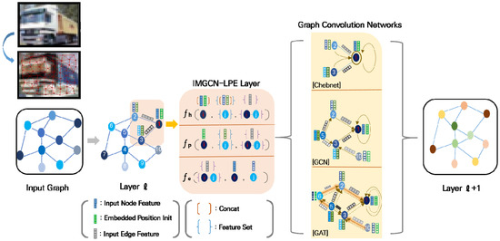
Instead of initially merging fixed positional information with structural information, we propose initializing the information separately and integrating it after learning. In this paper, we call this method IMGCN-LPE. The overall architecture of the IMGCN-LPE is depicted in Figure 2.

Figure 2. Main architecture of the graph convolutional network with learnable positional embedding applied on images (IMGCN-LPE).

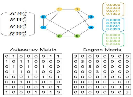
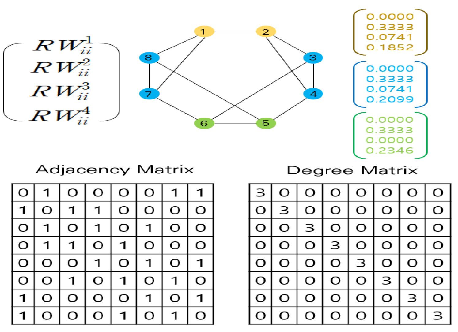
The procedure of initializing the positional information before supplying it in the IMGCN-LPE is essential. Initializing the positional information is defined based on a random walk ($RW)$, as presented in Equation (19), and the initial positional embedding at the input layer $l=0$ in Equation (20):

$$p_i^{RW}=\left\{R{W}_{ii}^1, R{W}_{ii}^2, \dots , R{W}_{ii}^k\right\},$$

(19)

$$p_i^{l=0}=L{L}_p(p_i^{RW})=D^0{p}_i^{RW}+d^0,$$

(20)

where the $RW$ operator is defined in Equation (21):

$$RW=\mathcal{A}{\mathcal{D}}^{-1}.$$

(21)

This paper considers only the probability of returning to itself through random steps on each node, which solves the direction problem of Laplacian-based positional embedding methods. If the embedding dimension $\mathbb{k}$ is sufficiently large, it is possible to express the unique graph topology by learning the broad positional information up to the node reached by $\mathbb{k}$ hops. Figure 3 illustrates an example of an RW-based initialization of positional embedding with $\mathbb{k}=4$.

Figure 3. Example of initialization of positional embedding based on the random walk algorithm ($\mathbb{k}=4)$.

The learning process of IMGCN-LPE is defined in Equation (22):

$$IMGCN-LPE :\{\begin{array}{c}{h}_i^{l+1}={ℱ}_h\left(\left[\begin{array}{c}{h}_i^l\\ p_i^l\end{array}\right], {\left\{\left[\begin{array}{c}{h}_j^l\\ p_j^l\end{array}\right]\right\}}_{j\in {\mathcal{N}}_i}, e_{ij}^l\right)\\ p_i^{l+1}={ℱ}_p(p_i^l, {\{p_j^l\}}_{j\in {\mathcal{N}}_i}, e_{ij}^l)\\ e_{ij}^{l+1}={ℱ}_e(h_i^l, h_j^l, e_{ij}^l)\end{array}.$$

(22)

The difference between IMGCN-LPE and the standard MP defined in Equation (18) is that it continues updating the feature and positional embedding using learned positional embedding $p_i^l$, initialized based on the RW in $l=0$. In addition, using an activation function, such as rectified linear unit (ReLU), for selecting the message-passing function is the same, but in the case of ${ℱ}_p$, $tanh$ is used to allow both positive and negative values for position coordinates.

3.4. ArcFace Loss Function

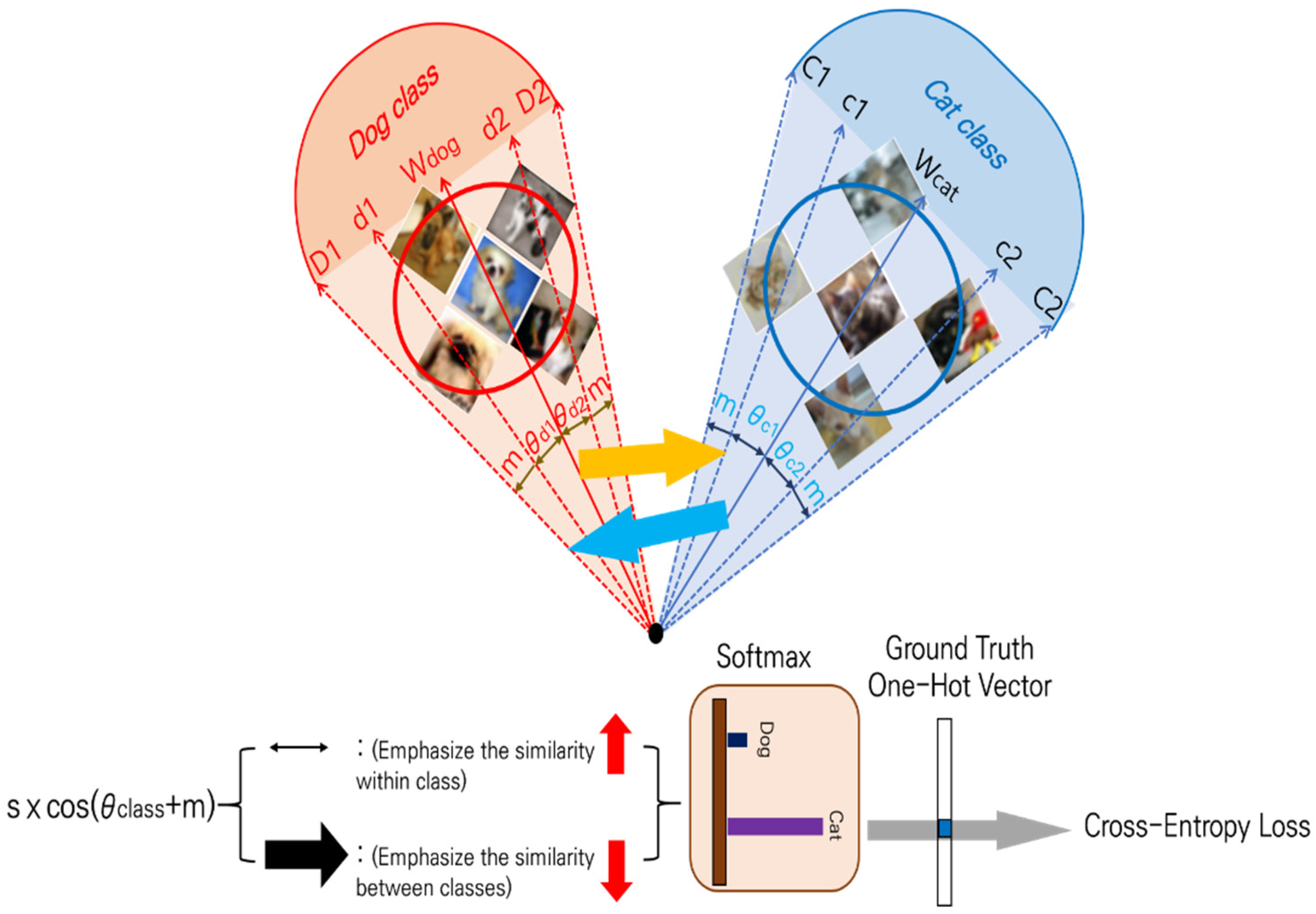
The ArcFace [32] loss function, primarily used in face recognition, focuses on the difference of angle between the class vector set $\mathcal{W}$ and data feature vector $𝓍$, minimizing it within the class and maximizing it among classes. In addition, the angle differences are further emphasized using the angular margin penalty (m) and scaling parameter (s), allowing GCNNs to learn boundary formations better between classes. The operation of ArcFace is presented in Figure 4.

Figure 4. Configuration of the ArcFace loss function.

Similarly to the HGNN, in this paper, we combined ArcFace and cross-entropy to define the final loss function ($\mathbb{L})$ in Equation (23):

$$\mathbb{L}=\alpha \times ArcFace+\beta \times CrossEntropy (\alpha \ne \beta ).$$

(23)

The main difference is that HGNN assigned the same weights as the loss functions, but we assigned different weights so that the learning process can concentrate on a specific loss function.

4. Experiments

In Section 4.1, we briefly summarize the basic information and preprocessing method about datasets we used for experiments. In the next Section 4.2, we present the experiment details about image preprocessing method and design of model architecture and hyper-parameters of experiments. Finally, in the last section (Section 4.3), we present the comparison of results of our proposed method with related studies and baseline GCNNs models and analysis of why the performance improved significantly on the results of ChebNet. In addition, we conclude the section by presenting the results of adding the ArcFace loss function.

4.1. Datasets

We experimented with the learnable positional embedding-based GCNNs performance on six benchmark datasets: FashionMNIST [41], CIFAR10 [42], SVHN [43], CAR196 [44], CUB200-2011 [45], and EuroSAT [46]. First, FashionMNIST is a grayscale image dataset of 10 kinds of fashion products with a size of 28 × 28 and consists of 60,000 training data and 10,000 testing data. Next, CIFAR10 is an RGB color-based image dataset of 10 categories with a size of 32 × 32, consisting of 50,000 training data and 10,000 testing data. The SVHN is an RGB street house-number image dataset divided into 10 numeric categories of 32 × 32 size and consists of 73,257 training data and 26,082 testing data. In addition, CAR196 is an RGB image dataset of 196 types of automobile brands with various sizes, consisting of 8041 training data and 8144 testing data. In the following dataset, we adjusted the image size equally to 224 × 224. Further, CUB200-2011 is an RGB image dataset of 200 kinds of birds of various sizes, consisting of 5794 training data and 8994 testing data. In this case, we adjusted the image sizes to 64 × 64 and 128 × 128. Finally, EuroSAT is a dataset of 27,000 Sentinel-2 satellite RGB-based 64 x 64 images divided into 10 categories. We split this dataset into 80% training data (approximately 21,600) and 20% testing data (approximately 5400).

In this paper, we compare the graph-represented superpixel image classification results with the state-of-the-art paper using the same dataset. Both FashionMNIST and CIFAR10 are compared with RAG-GAT [8], DISCO-GCN [35], and HGNN [10], whereas SVHN and EuroSAT are compared to RAG-GAT and HGNN, respectively. Moreover, CAR196 and CUB200-2011 compare the results of the IMGCN-LPE with the baseline models (ChebNet [29], GCN [5], and GAT [30]) because we could not find a paper that provided results on the same datasets.

4.2. Experiment Details

In this paper, when segmenting the benchmark images to superpixels, we equally used the SLIC algorithm and generated 75 superpixel regions. All baseline models initialize the positional vector of all nodes based on the RW algorithm. The vector dimension $\mathbb{k}$ was set to the same value as the Chebyshev polynomial order $K$ for ChebNet and was set to a fixed value of 4 for the GCN and GAT.

The configuration of the baseline model is described as follows. Similar to all datasets, ChebNet has two graph convolutional layers consisting of aggregating the information for $K$ hop nodes and the ReLU activation function and a graph max-pooling layer in order after passing the last convolution layer. In addition, it has two fully connected layers and has class prediction accuracy based on the softmax regression classifier.

Unlike ChebNet, we designed a different GCN configuration for one-channel and three-channel datasets. The FashionMNIST dataset is passed two graph convolutional layers based on the MP and the readout layer defined as the mean function, graph max-pooling layer, and fully connected layer in order. Furthermore, its accuracy is based on the softmax regression classifier. The other RGB datasets are passed four graph convolutional layers, mean-readout, graph max-pooling, and three fully connected layers to obtain a result.

The GAT, similar to all datasets, has two layers of graph convolution based on two multihead attention mechanisms and readout layers, defined by the sum function, and passes the multilayer perceptron as a fully connected layer to obtain the results.

The learning procedures of the baseline models with the learnable positional embedding method are provided in Equations (24)–(26) in the order of the ChebNet, GCN, and GAT:

$$\mathit{Cheb}-\mathit{LPE}:\{\begin{array}{c}{h}_i^{l+1}=ReLU\left(BN\left(\left[A_1^l\left[ \begin{array}{c}{h}_i^l\\ p_i^l\end{array} \right], \left({\displaystyle {\displaystyle \sum }_{k=1}^{K-1}}{A}_2^l\left[ \begin{array}{c}{h}_k^l\\ p_k^l\end{array} \right]\right)\right]\right)\right)\\ e_{ij}^{l+1}=ReLU (BN({\displaystyle {\displaystyle \sum }_{k=1}^{K-1}}(B_2^l{e}_{ik}^l)), \\ p_i^{l+1}=\text{tanh}(C_1^l{p}_i^l+{{\displaystyle \sum }}_{j\in {\mathcal{N}}_i}{C}_2^l{p}_j^l)\end{array}$$

(24)

$$GCN-LPE: \{\begin{array}{c}{h}_i^{l+1}=ReLU(BN(A_1^l\left[\begin{array}{c}{h}_i^l\\ p_i^l\end{array}\right]+{{\displaystyle \sum }}_{j\in {\mathcal{N}}_i}{A}_2^l\left[\begin{array}{c}{h}_j^l\\ p_j^l\end{array}\right])),\\ e_{ij}^{l+1}=ReLU(BN(B_1^l{h}_i^l+B_2^l{h}_j^l+e_{ij}^l)), \\ p_i^{l+1}=\tanh (C_1^l{p}_i^l+{{\displaystyle \sum }}_{j\in {\mathcal{N}}_i}{C}_2^l{p}_j^l)\end{array}$$

(25)

$$\mathit{GAT}-\mathit{LPE}:\{\begin{array}{c}{e}_{ij}=\overrightarrow{a}(A_1^l\left[\begin{array}{c}{h}_i^l\\ p_i^l\end{array}\right], A_2^l\left[\begin{array}{c}{h}_j^l\\ p_j^l\end{array}\right]), {\alpha }_{ij}=Softmax(e_{ij})\\ h_i^{l+1}=ELU(\frac{1}{K}{\displaystyle {\displaystyle \sum }_{k=1}^K}{{\displaystyle \sum }}_{j\in {\mathcal{N}}_i}{\alpha }_{ij}^k{A}_2^l{h}_j^l),\\ e_{ij}^{l+1}=ReLU(BN(B_1^l{h}_i^l+B_2^l{h}_j^l+B_3^l{e}_{ij}^l)\\ p_i^{l+1}=\text{tanh}(C_1^l{p}_i^l+{{\displaystyle \sum }}_{j\in {\mathcal{N}}_i}{C}_2^l{p}_j^l)\end{array}$$

(26)

where BN denotes batch normalization.

We set the hyperparameters that the epoch was 100, the batch size was 64, the learning rate was 0.001, and the dropout rate was 0.5. For optimization, we used the stochastic gradient descent [47] with a momentum of 0.9 for ChebNet and Adam [48] with a weight decay of 0.95 for the GCN and GAT. In addition, the scale parameter (s) and the angular margin penalty (m) were set to 64 and 0.5 radian (approximately 29°), respectively. The weight of ArcFace was set to 0.2.

4.3. Results Details

The results of SLIC and IMGCN-LPE for the six benchmark image datasets are listed in Table 1, and the best results are marked in bold. When the baseline model is ChebNet, the performance decreases significantly when the superpixel images are supplied because the filter of ChebNet is isotropic. The concept of direction does not exist, and it cannot clearly distinguish the different graphs represented in each image. However, in the case of IMGCN-LPE, the filter has obtained orientation by continuously learning positional information in training and can understand the graph topology in a broad context so that the power of distinguishing various graph structures increases and achieves better results.

Table 1. Detailed experimental results of baseline models (Chebyshev graph convolutional network (ChebNet) of aggregating maximum K = 25 neighbors information, graph convolutional network(GCN) with stacking single layer (1Layer) or two layers (2Layers), and graph attention network (GAT) with single head (1Head) or two multi-heads attention (2Heads)) and IMGCN-LPE applied to SLIC-75 images.

Preprocess	Model	Dataset
		F-MNIST (28 × 28)	CIFAR10 (32 × 32)	SVHN (32 × 32)	CAR196 (224 × 224)	CUB200 (64 × 64)	CUB200 (128 × 128)	EuroSAT (64 × 64)
SLIC-75	GCN-1Layer	87.542	46.497	72.682	51.498	58.477	58.070	66.487
	GCN-2Layers	89.794	57.219	73.454	53.842	62.813	63.466	67.921
	GAT-1Head	89.688	57.693	79.211	58.903	65.813	67.544	71.608
	GAT-2Heads	90.874	61.103	80.726	59.582	67.560	69.620	74.863
	ChebNet (K = 25)	79.167	33.297	52.045	27.663	47.093	45.647	54.236
	IMGCN-LPE
	GCN-1Layer	89.183	50.563	74.133	55.712	61.916	64.866	65.736
	GCN-2Layers	90.561	60.464	75.486	57.808	65.848	67.212	66.388
	GAT-1Head	90.618	66.480	80.511	61.438	68.223	69.838	74.758
	GAT-2Heads	92.013	68.632	81.986	62.729	70.192	72.101	76.373
	ChebNet (K = 25)	91.21	73.086	80.714	60.861	70.484	69.637	75.482

The comparison of the experimental results with the related work is presented in Table 2. Compared to the previous state-of-the-art models, the IMGCN-LPE method in FashionMNIST is about 2% higher than the DISCO-GCN, about 2.5% higher than the HGNN in CIFAR10, and about 1.2% higher than the HGNN in EuroSAT. For CAR196 and CUB200-2011, IMGCN-LPE is better by about 1.9% to 2.5% compared to the baseline models.

Table 2. Comparison of the experimental results with related studies.

Method	Model	Dataset
		F-MNIST (28 × 28)	CIFAR10 (32 × 32)	SVHN (32 × 32)	CAR196 (224 × 224)	CUB200 (64 × 64)	CUB200 (128 × 128)	EuroSAT (64 × 64)
SLIC-75	RAG-GAT	83.07	45.93	80.72	-	-	-	-
	DISCO-GCN	90.02	70.01	-	-	-	-	-
	HGNN	-	70.61	-	-	-	-	75.22
	GCN-2Layers	-	-	-	53.84	62.81	63.49	-
	GAT-2Heads	-	-	-	59.58	67.56	69.62	-
	IMGCN-LPE
	Baseline models	92.01	73.09	81.99	62.73	70.48	72.10	76.37

When determining the final loss function, experimentally, a higher weight for the cross-entropy loss function provides better results. Compared to using just cross-entropy, the performance improves by about 0.2% to 5.3%. The experimental results with the 0.2 weighted ArcFace loss function are presented in Table 3.

Table 3. Experimental results of ChebNet, GCN, and GAT after adding the ArcFace loss function with a weight of 0.2.

Preprocess	Model	Dataset
		F-MNIST (28 × 28)	CIFAR10 (32 × 32)	SVHN (32 × 32)	CAR196 (224 × 224)	CUB200 (64 × 64)	CUB200 (128 × 128)	EuroSAT (64 × 64)
SLIC-75	IMGCN-LPE
	GCN-1Layer	89.18 → 89.32	50.56 → 55.85	74.13 → 75.38	55.71 → 55.79	61.92 → 63.01	65.74 → 65.93	65.74 → 66.04
	GCN-2Layers	90.56 → 90.98	60.46 → 60.84	75.47 → 76.61	57.61 → 57.88	65.85 → 65.92	67.21 → 67.74	66.39 → 66.77
	GAT-1Head	90.62 → 90.90	66.46 → 67.28	80.51 → 81.17	61.44 → 61.76	68.22 → 69.06	69.90 → 72.45	74.76 → 74.96
	GAT-2Heads	92.01 → 92.25	68.63 → 69.71	81.99 → 82.52	62.73 → 63.46	70.19 → 70.62	72.10 → 73.85	76.37 → 76.96
	ChebNet (K = 25)	91.21 → 91.63	73.09 → 73.22	80.71 → 82.02	60.86 → 61.20	70.48 → 72.99	69.64 → 71.26	75.48 → 76.61

5. Conclusions

In this paper, we present a new approach to the problem of superpixel image classification based on GCNNs. Using an SLIC algorithm, the distance between pixels is calculated based on each positional coordinate and is segmented into a specific number of superpixels. The RAG algorithm creates a graph using the central coordinates as new positional information for each region. However, it is not robust to various graph structures due to the fixed positional information defined by the central coordinates, which is the main issue of the degradation of the ability of the GCNNs.

The IMGCN-LPE method we proposed makes GCNNs powerful enough to extend its coverage to various graph structures by continuously learning the positional property. As shown by the experiment results of various benchmark image datasets, it outperforms other related work on various benchmark image datasets that improve about 1.2% to 2.5% of accuracy. In addition, it is confirmed that adding ArcFace to the cross-entropy as loss function increases performance about 0.2% to a maximum of 5.3% more.

Although the proposed method does not perform as impressively as the CNN, it can provide a useful framework for graph representation-based computer vision tasks. Moreover, it is also a good indicator for more advanced ideas regarding more complicated visual issues in the future.

References

- He, K.; Zhang, X.; Ren, S.; Sun, J. Deep residual learning for image recognition. In Proceedings of the IEEE Conference on Computer Vision and Pattern Recognition, Las Vegas, NV, USA, 27–30 June 2016; pp. 770–778. [Google Scholar]
- Krizhevsky, A.; Sutskever, I.; Hinton, G.E. Imagenet classification with deep convolutional neural networks. Commun. ACM 2017, 60, 84–90. [Google Scholar] [CrossRef]
- Simonyan, K.; Zisserman, A. Very deep convolutional networks for large-scale image recognition. arXiv 2014, arXiv:1409.1556. [Google Scholar]
- Pasdeloup, B.; Gripon, V.; Vialatte, J.C.; Pastor, D.; Frossard, P. Convolutional neural networks on irregular domains based on approximate vertex-domain translations. arXiv 2017, arXiv:1710.10035. [Google Scholar]
- Kipf, T.N.; Welling, M. Semi-supervised classification with graph convolutional networks. arXiv 2016, arXiv:1609.02907. [Google Scholar]
- Xu, K.; Hu, W.; Leskovec, J.; Jegelka, S. How powerful are graph neural networks? arXiv 2018, arXiv:1810.00826. [Google Scholar]
- Monti, F.; Boscaini, D.; Masci, J.; Rodola, E.; Svoboda, J.; Bronstein, M.M. Geometric deep learning on graphs and manifolds using mixture model cnns. In Proceedings of the IEEE Conference on Computer Vision and Pattern Recognition, Honolulu, HI, USA, 21–26 July 2017. [Google Scholar]
- Avelar, P.H.; Tavares, A.R.; da Silveira, T.L.; Jung, C.R.; Lamb, L.C. November. Superpixel image classification with graph attention networks. In Proceedings of the 33rd SIBGRAPI Conference on Graphics, Patterns and Images (SIBGRAPI), Porto de Galinhas, Brazil, 7–10 November 2020. [Google Scholar]
- Bae, J.H.; Vu, D.T.; Kim, J.Y. Superpixel Image Classification based on Graph Neural Network. In Proceedings of the Korea Telecommunications Society Conference, Pyeongchang, Korea, 9–11 February 2022; pp. 971–972. [Google Scholar]
- Long, J.; Yan, Z.; Chen, H. A Graph Neural Network for superpixel image classification. J. Phys. Conf. Ser. 2021, 1871, 012071. [Google Scholar] [CrossRef]
- Dadsetan, S.; Pichler, D.; Wilson, D.; Hovakimyan, N.; Hobbs, J. Superpixels and Graph Convolutional Neural Networks for Efficient Detection of Nutrient Deficiency Stress from Aerial Imagery. In Proceedings of the IEEE/CVF Conference on Computer Vision and Pattern Recognition, virtual, 19–25 June 2021; pp. 2950–2959. [Google Scholar] [CrossRef]
- Wang, K.; Li, L.; Zhang, J. End-to-end trainable network for superpixel and image segmentation. Pattern Recognit. Lett. 2020, 140, 135–142. [Google Scholar] [CrossRef]
- Yang, C.; Zhang, L.; Lu, H.; Ruan, X.; Yang, M.H. Saliency detection via graph-based manifold ranking. In Proceedings of the IEEE Conference on Computer Vision and Pattern Recognition, Portland, OR, USA, 23–28 June 2013; pp. 3166–3173. [Google Scholar]
- Zhang, K.; Li, T.; Shen, S.; Liu, B.; Chen, J.; Liu, Q. Adaptive graph convolutional network with attention graph clustering for co-saliency detection. In Proceedings of the IEEE/CVF Conference on Computer Vision and Pattern Recognition, Seattle, WA, USA, 13–19 June 2020; pp. 9050–9059. [Google Scholar]
- Diao, Q.; Dai, Y.; Zhang, C.; Wu, Y.; Feng, X.; Pan, F. Superpixel-Based Attention Graph Neural Network for Semantic Segmentation in Aerial Images. Remote Sens. 2022, 14, 305. [Google Scholar] [CrossRef]
- Mentasti, S.; Matteucci, M. Image Segmentation on Embedded Systems via Superpixel Convolutional Networks. In Proceedings of the European Conference on Mobile Robots (ECMR), Prague, Czech Republic, 4–6 September 2019; pp. 1–7. [Google Scholar]
- Zhang, C.; Lin, G.; Liu, F.; Guo, J.; Wu, Q.; Yao, R. Pyramid graph networks with connection attentions for region-based one-shot semantic segmentation. In Proceedings of the IEEE/CVF International Conference on Computer Vision, Seoul, Korea, 27 October–2 November 2019; pp. 9587–9595. [Google Scholar]
- Schlichtkrull, M.; Kipf, T.N.; Bloem, P.; Van Den Berg, R.; Titov, I.; Welling, M. Modeling Relational Data with Graph Convolutional Networks. In European Semantic Web Conference; Springer: Berlin/Heidelberg, Germany, 2018; pp. 593–607. [Google Scholar] [CrossRef]
- Pradhyumna, P.; Shreya, G.P. Graph neural network (GNN) in image and video understanding using deep learning for computer vision applications. In Proceedings of the Second International Conference on Electronics and Sustainable Communication Systems (ICESC), Coimbatore, India, 4–6 August 2021; pp. 1183–1189. [Google Scholar]
- Wu, L.; Chen, Y.; Shen, K.; Guo, X.; Gao, H.; Li, S.; Pei, J.; Long, B. Graph neural networks for natural language processing: A survey. arXiv 2021, arXiv:2106.06090. [Google Scholar]
- Zhong, T.; Wang, T.; Wang, J.; Wu, J.; Zhou, F. Multiple-Aspect Attentional Graph Neural Networks for Online Social Network User Localization. IEEE Access 2020, 8, 95223–95234. [Google Scholar] [CrossRef]
- Li, Y.; Ji, Y.; Li, S.; He, S.; Cao, Y.; Liu, Y.; Liu, H.; Li, X.; Shi, J.; Yang, Y. Relevance-aware anomalous users detection in social network via graph neural network. In Proceedings of the International Joint Conference on Neural Networks (IJCNN), Shenzhen, China, 18–22 July 2021; pp. 1–8. [Google Scholar]
- Wang, Y.; Wang, J.; Cao, Z.; Farimani, A.B. Molclr: Molecular contrastive learning of representations via graph neural networks. arXiv 2021, arXiv:2102.10056. [Google Scholar]
- Godwin, J.; Schaarschmidt, M.; Gaunt, A.L.; Sanchez-Gonzalez, A.; Rubanova, Y.; Veličković, P.; Kirkpatrick, J.; Battaglia, P. Simple gnn regularisation for 3d molecular property prediction and beyond. In Proceedings of the International Conference on Learning Representations, Virtual Event, 3–7 May 2021. [Google Scholar]
- Achanta, R.; Shaji, A.; Smith, K.; Lucchi, A.; Fua, P.; Süsstrunk, S. SLIC superpixels compared to state-of-the-art superpixel methods. IEEE Trans. Pattern Anal. Mach. Intell. 2012, 34, 2274–2282. [Google Scholar] [CrossRef] [PubMed]
- Vedaldi, A.; Soatto, S. Quick shift and kernel methods for mode seeking. In Proceedings of the European Conference on Computer Vision, Marseille, France, 12–18 October 2008; pp. 705–718. [Google Scholar]
- Felzenszwalb, P.F.; Huttenlocher, D.P. Efficient graph-based image segmentation. Int. J. Comput. Vis. 2004, 59, 167–181. [Google Scholar] [CrossRef]
- Bruna, J.; Zaremba, W.; Szlam, A.; LeCun, Y. Spectral networks and locally connected networks on graphs. arXiv 2013, arXiv:1312.6203. [Google Scholar]
- Defferrard, M.; Bresson, X.; Vandergheynst, P. Convolutional neural networks on graphs with fast localized spectral filtering. In Advances in Neural Information Processing Systems 29 (NIPS 2016); Curran Associates, Inc.: Red Hook, NY, USA, 2017; Volume 29. [Google Scholar]
- Veličković, P.; Cucurull, G.; Casanova, A.; Romero, A.; Lio, P.; Bengio, Y. Graph attention networks. arXiv 2017, arXiv:1710.10903. [Google Scholar]
- Dwivedi, V.P.; Luu, A.T.; Laurent, T.; Bengio, Y.; Bresson, X. Graph neural networks with learnable structural and positional representations. arXiv 2021, arXiv:2110.07875. [Google Scholar]
- Deng, J.; Guo, J.; Xue, N.; Zafeiriou, S. Arcface: Additive angular margin loss for deep face recognition. In Proceedings of the IEEE/CVF Conference on Computer Vision and Pattern Recognition, Long Beach, CA, USA, 15–20 June 2019; pp. 4690–4699. [Google Scholar]
- Vaswani, A.; Shazeer, N.; Parmar, N.; Uszkoreit, J.; Jones, L.; Gomez, A.N.; Kaiser, Ł.; Polosukhin, I. Attention is all you need. In Advances in Neural Information Processing Systems 30 (NIPS 2017); Curran Associates, Inc.: Red Hook, NY, USA, 2017; Volume 30. [Google Scholar]
- LeCun, Y. The MNIST Database of Handwritten Digits. 1998. Available online: http://yann.lecun.com/exdb/mnist/ (accessed on 4 August 2022).
- Youn, C.H. Dynamic graph neural network for super-pixel image classification. In Proceedings of the International Conference on Information and Communication Technology Convergence (ICTC), Jeju Island, Korea, 20–22 October 2021; pp. 1095–1099. [Google Scholar]
- De Boer, P.T.; Kroese, D.P.; Mannor, S.; Rubinstein, R.Y. A tutorial on the cross-entropy method. Ann. Oper. Res. 2005, 134, 19–67. [Google Scholar] [CrossRef]
- Dwivedi, V.P.; Bresson, X. A generalization of transformer networks to graphs. arXiv 2020, arXiv:2012.09699. [Google Scholar]
- Dwivedi, V.P.; Joshi, C.K.; Laurent, T.; Bengio, Y.; Bresson, X. Benchmarking graph neural networks. arXiv 2020, arXiv:2003.00982. [Google Scholar]
- Li, P.; Wang, Y.; Wang, H.; Leskovec, J. Distance encoding: Design provably more powerful neural networks for graph representation learning. In Advances in Neural Information Processing Systems 33 (NIPS 2020); Curran Associates, Inc.: Red Hook, NY, USA, 2020; Volume 33, pp. 4465–4478. [Google Scholar]
- You, J.; Ying, R.; Leskovec, J. Position-aware graph neural networks. In Proceedings of the International Conference on Machine Learning, Long Beach, CA, USA, 10–15 June 2019; pp. 7134–7143. [Google Scholar]
- Xiao, H.; Rasul, K.; Vollgraf, R. Fashion-mnist: A novel image dataset for benchmarking machine learning algorithms. arXiv 2017, arXiv:1708.07747. [Google Scholar]
- Krizhevsky, A.; Hinton, G. Learning Multiple Layers of Features from Tiny Images; University of Toronto: Toronto, ON, Canada, 2009. [Google Scholar]
- Netzer, Y.; Wang, T.; Coates, A.; Bissacco, A.; Wu, B.; Ng, A.Y. Reading digits in natural images with unsupervised feature learning. In Proceedings of the NIPS Workshop on Deep Learning and Unsupervised Feature Learning, Granada, Spain, 12–17 December 2011. [Google Scholar]
- Krause, J.; Stark, M.; Deng, J.; Fei-Fei, L. 3d object representations for fine-grained categorization. In Proceedings of the IEEE International Conference on Computer Vision Workshops, Sydney, NSW, Australia, 2–8 December 2013; pp. 554–561. [Google Scholar]
- Wah, C.; Branson, S.; Welinder, P.; Perona, P.; Belongie, S. The Caltech-UCSD Birds-200-2011 Dataset; California Institute of Technology: Pasadena, CA, USA, 2011. [Google Scholar]
- Helber, P.; Bischke, B.; Dengel, A.; Borth, D. EuroSAT: A Novel Dataset and Deep Learning Benchmark for Land Use and Land Cover Classification. IEEE J. Sel. Top. Appl. Earth Obs. Remote Sens. 2019, 12, 2217–2226. [Google Scholar] [CrossRef]
- Bottou, L. Large-Scale Machine Learning with Stochastic Gradient Descent. In Proceedings of the 19th International Conference on Computational Statistics, Paris, France, 22–27 August 2010; pp. 177–186. [Google Scholar] [CrossRef] [Green Version]
- Kingma, D.P.; Ba, J. Adam: A method for stochastic optimization. arXiv 2014, arXiv:1412.6980. [Google Scholar]
Publisher’s Note: MDPI stays neutral with regard to jurisdictional claims in published maps and institutional affiliations. |
© 2022 by the authors. Licensee MDPI, Basel, Switzerland. This article is an open access article distributed under the terms and conditions of the Creative Commons Attribution (CC BY) license (https://creativecommons.org/licenses/by/4.0/).