DeConNet: Deep Neural Network Model to Solve the Multi-Job Assignment Problem in the Multi-Agent System

Abstract

In a multi-agent system, multi-job assignment is an optimization problem that seeks to minimize total cost. This can be generalized as a complex problem in which several variations of vehicle routing problems are combined, and as an NP-hard problem. The parameters considered include the number of agents and jobs, the loading capacity, the speed of the agents, and the sequence of consecutive positions of jobs. In this study, a deep neural network (DNN) model was developed to solve the job assignment problem in a constant time regardless of the state of the parameters. To generate a large training dataset for the DNN, the planning domain definition language (PDDL) was used to describe the problem, and the optimal solution that was obtained using the PDDL solver was preprocessed into a sample of the dataset. A DNN was constructed by concatenating the fully-connected layers. The assignment solution obtained via DNN inference increased the average traveling time by up to 13% compared with the ground cost. As compared with the ground cost, which required hundreds of seconds, the DNN execution time was constant at approximately 20 ms regardless of the number of agents and jobs.

1. Introduction

In a multi-agent system, the job assignment problem between multiple agents and jobs is a combinational optimization problem that minimizes the total cost of the traveling time or distance.

There are multiple agents and jobs in the job assignment problem, and each agent and job is in a specific two-dimensional position. Each agent has a different movement speed and loading capacity for the allocated job. A job is an ordered sequence that results in movement from a starting position to a target position. Agents can select several jobs that are within their loading capacity. A robot, for example, may move multiple objects, or a worker may receive multiple delivery requests. When all the jobs have been moved to their target location and are completed, the allocation between the agents and the jobs aims to minimize the sum of the time spent traveling, which is calculated based on each agent’s moving speed, or the time spent on the last completed task.

This multi-parameter allocation problem can be generalized as the vehicle routing problem (VRP). Since the VRP was first proposed [1], VRP with pickup and delivery (VRPPD) [2,3], capacitated VRP (CVRP) [4], open VRP (OVRP) [5], multi-depot VRP (MDVRP) [6,7], and many other variants have been investigated.

An agent in VRPPD must handle multiple sequential jobs from specific start (pickup) locations to other destination (delivery) locations. In the CVRP, each agent with the same capacity is assigned a set of jobs to achieve minimum-cost routes that originate and terminate at a depot. The OVRP is similar to the CVRP, but unlike the CVRP, an agent does not have to return to a depot. As a result, the route terminates when the last job is completed. The MDVRP extends the CVRP by allowing depots to be placed in multiple locations.

This study’s allocation problem is a combination of all of the aforementioned conditions, which reflect a real-world scenario. Based on the problem definition, all jobs should be selected only once; one job only moves from the starting position to the target position; multiple agents can select and process any number of jobs; and there is no need to return to the agent’s starting position when the jobs have been completed. Therefore, this can be regarded as a variation of the vehicle routing problem wherein an open VRP in which vehicles with different loading capacity limitations start from multiple depots pick up at a specific location in the job and deliver to another location, and the pickup of other jobs may occur between the pickup and delivery of a job. This is an NP-hard problem known as the multi-depot capacitated open vehicle routing problem with pickup and delivery (MDCOVRPPD).

In previous studies that applied a metaheuristic algorithm to VRP variants such as MDVRP or VRPPD, the computation time increased by hundreds of seconds as the number of agents and jobs increased [8,9,10]. As such, the direct application of the algorithm to problem-solving in a real-world environment is difficult.

In this study, we designed a deep neural network (DNN) that infers a result close to the optimal solution to solve the subproblem with a time complexity of $O\left(1\right)$ for the MDCOVRPPD that considers several complex parameters. The results indicate that the proposed approach can be applied to real-world scenarios by solving the allocation problem within a specified time (e.g., tens of microseconds). The number of input agents and jobs for the inference of a DNN is limited owing to the limitations of the computing resources used in this study. Many agents and jobs in the real world are handled by subsets using divide-and-conquer methods.

The following is a summary of the study’s contributions:

• This study entailed the development of a DNN model for solving the assignment problem between multiple agents and multiple jobs in a variant of the VRP with real-world parameters. As compared to the previously proposed methods, the proposed method executes quickly without sequential procedures.
• We devised a method for generating a dataset for training the proposed deep neural network model by using the planning domain definition language (PDDL). Various parameter types were defined and relationships between parameters were expressed in the PDDL description of the domain. By running the solver, a large number of data samples can be acquired from multiple PDDL problem descriptions with different initial values and goals.

In this paper, related works are discussed in Section 2. Section 3 defines the job assignment problem and describes the implementation of the PDDL to generate assignments based on global search, which is created by varying multiple parameters in many instances. Section 4 describes the DNN structure and the specification of the training dataset. Section 5 outlines the proposed DNN inference result by comparing it with the ground cost. Finally, in Section 6 we present the main conclusions and outline our future work.

2. Related Works

In this section, we briefly survey related studies, including VRP variants, PDDL, and machine learning for solving the assignment problem.

2.1. Vehicle Routing Problem and Variants

The VRP is defined as the optimal set of routes for a fleet of vehicles and agents that travel to perform delivery to a given customer. This is referred to as a combinational integer optimization problem [11]. The VRP is a generalization of the traveling salesman problem; as it is NP-Hard, polynomial-time algorithms are unlikely to exist unless $P=NP$. Despite the computational complexity of these problems, novel heuristic methods are able to obtain near-optimal solutions within seconds for a few specific datasets.

There are several VRP variants [12,13,14] as follows:

• Multi-depot vehicle routing problem (MDVRP): In this variant, multiple vehicles leave from different depots and return to their original depots at the end of their assigned jobs.
• Capacitated vehicle routing problem (CVRP): This variant is a particular case of the MDVRP in which the number of depots is one. Each vehicle has a limited carrying capacity.
• Vehicle routing problem with pickup and delivery (VRPPD): Several items/jobs must be moved/processed from certain pickup locations to other delivery locations. The objective of the VRPPD is to determine a set of optimal routes for the vehicle to visit the pickup and delivery locations.
• Open vehicle routing problem (OVRP): In this variant, the vehicle does not have to return to the depot.

Given that methods with exact solutions such as vehicle flow formulations, commodity flow formulations, and set partitioning problems [15] generally fail to solve real-world problems within feasible computation time frames, the emphasis of VRP solution methods has shifted to heuristic approaches. However, there is no guarantee of quality solutions.

Heuristic algorithms for VRP can be categorized into constructive and improvement methods. Constructive methods are typically quick, greedy approaches. Improvement methods are more sophisticated and typically require a VRP solution as the input [16]. Well-known constructive methods for VRP include the nearest neighbor heuristic algorithm, sweep algorithm [17], and the cluster-first path-second method [18]. Heuristic improvement methods utilize a strategy called metaheuristics, iteratively moving from one solution to a new solution via modifications. The metaheuristics for the VRP include simulated annealing [19], tabu search [20], genetic algorithms [21], memetic algorithms [22], and neural networks [23].

2.2. Planning Domain Definition Language

The PDDL is an action-oriented language inherited from the well-known STRIPS [24] formulations of planning problems [25]. It implements a simple standardization of the syntax for expressing this behavioral semantics, which uses pre- and post-conditions to describe the applicability and effectiveness of behaviors. A planning problem is represented by the pairing of a domain description with a problem description. A domain description is sometimes coupled with many different problem descriptions to create different planning problems. An instance of a problem description includes the parameterized actions that characterize domain behaviors based on the description of objects, initial conditions, and goals. The pre- and post-conditions of actions are expressed as logical sentences constructed from predicates, arguments, and logical operators. In [26,27,28], PDDL models were developed for several VRP variants, such as CVRP and VRPTW, and their performances were compared.

2.3. Machine Learning for Solving the Assignment Problem

Recently, with advances in machine learning methodologies, many researchers have attempted to solve combinatorial optimization problems using only methods based on this approach, without mathematical models or metaheuristic algorithms.

In one study [29], to solve a large-scale VRP, a training dataset was created by merging several outputs that were computed using a heuristic solver based on small, partitioned problem instances with approximately 100 jobs/cities. Using the machine learning model, the execution time was reduced from tens of minutes to several seconds, while maintaining a similar cost compared to the previous heuristic solver.

In another study [30], the linear sum assignment problem was decomposed into multiple sub-assignment problems, allowing for the reconstruction of the problem to classify subproblems and simultaneously reduce the size of the DNN. The accuracy of the DNN model of the feed-forward neural network was approximately 10% lower than that of the Hungarian algorithm. However, the execution time was reduced by 1%.

3. Definition and PDDL Description of the Job Assignment Problem between Multiple Agents and Multiple Jobs

3.1. Problem Definition for MDCOVRPPD

There are many agents ($W_j, j=1,2,\dots ,m$), and many jobs ($J_k, k=1,2,\dots ,n$) are arranged in two-dimensional space. In the initial position, the agent (W_j) has a moving speed (V_j), energy level (B_j), residual performance (R_j), and maximum loading capacity (L_j) for multiple job selections. Job ($J_k$) is a sequence that moves from the starting position ($S_k$) to the target position ($T_k$), and a sequence of other jobs may overlap during the execution of the sequence of a job. All jobs must be selected and processed, but not all agents must do the job. The agent may select fewer jobs than their maximum loading capacity and, in some cases, may not select any jobs. The agent can move to the target position of the current job or the starting position of another job after arriving at the starting position of the selected job. According to this selection, the time of travel was calculated as the distance between the positions divided by the moving speed of each agent.

In the case of a general CVRP, the parameters that define the problem are the number of customers/jobs ($N$), the number of vehicles/agents ($K$), and the capacity of the vehicle/agent ($C$). ($C$) has a fixed value based on ($N$) and ($K$).

In contrast, the parameters considered in the instance of MDCOVRPPD are the number of jobs ($N$), number of agents ($K$), payload loading capacity of an agent ($L$), velocity of an agent ($V$), starting position of a job ($S$), target position of a job ($T$), energy level of an agent ($B$), and residual performance of an agent (R). When creating each problem instance, all parameters were randomly generated within a specified range, except for ($N$) and ($K$).

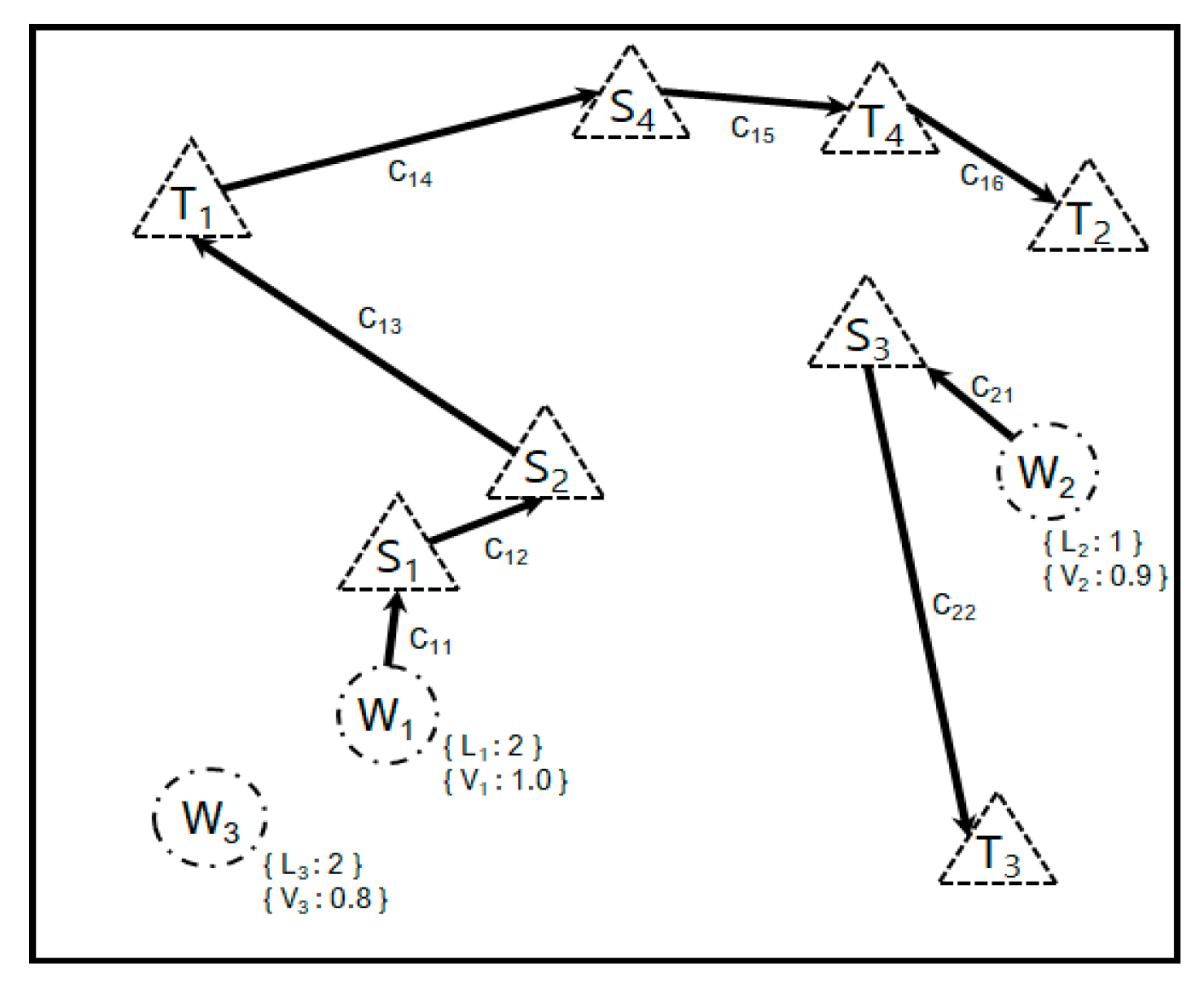
Figure 1 shows an example of a job assignment. When the number of agents is three and the number of jobs is four, job $\left\{J_1, J_2, J_4\right\}$ is assigned to agent $\left\{W_1\right\}$, job $\left\{J_3\right\}$ is assigned to agent $\left\{W_2\right\}$, and agent $\left\{W_3\right\}$ is not assigned a job.

Figure 1. An example of the multi-agent (M = 3) and multi-job (N = 4) assignment problem.

If agent $W_i$ selects $N$ jobs, the maximum number of state transitions is calculated in Equation (1) as follows:

$$\#MA{X}_{TR}{\left.\right|}_{W_i}=N\ast \left(N+1\right)\ast \left(N-1\right)!=\left(N+1\right)!$$

(1)

The actual number of state transitions is smaller than that of Equation (1) because the target position in which the starting position is not selected in the sequence for the state transition cannot be changed.

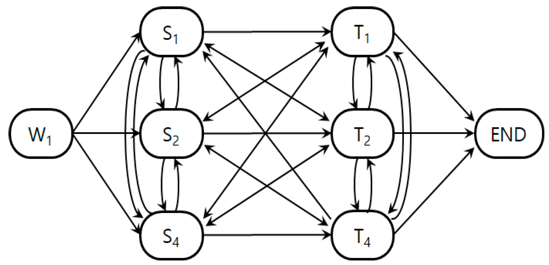
Figure 2 shows an example of a state transition diagram. Agent $W_1$ can display a path of state transitions that can be selected for three jobs $\left\{J_1\left(S_1\to T_1\right),J_2\left(S_2\to T_2\right),J_4\left(S_4\to T_4\right)\right\}$.

Figure 2. An example of a state-transition diagram for 3 jobs by a worker.

The sparse state-transition matrix $M$ for the moving path of agent $W_1$ is illustrated in Figure 3. The values of gray and blank in the matrix are zero ($M_{ij}=0$).

Figure 3. An example of a sparse state-transition matrix M.

The total cost of the agent $W_1$’s traveling path is as shown in Equations (2) and (3).

$$\begin{array}{ll}totalcost& {\left.\right|}_{W_1}=\sum c\left(T{r}_i,T{r}_j\right){\left.\right|}_{W_1}\\ & =\mathrm{c}\left(W_1,S_1\right){\left.\right|}_{W_1}+c\left(S_1,S_2\right){\left.\right|}_{W_1}+c\left(S_2,T_1\right){\left.\right|}_{W_1}+\\ & c\left(T_1,S_4\right){\left.\right|}_{W_1}+c\left(S_4,T_4\right){\left.\right|}_{W_1}+c\left(T_4,T_2\right){\left.\right|}_{W_1}+\\ & c\left(T_2,END\right){\left.\right|}_{W_1}\end{array}$$

(2)

$$c\left(T{r}_i,T{r}_j\right){\left.\right|}_{{\mathrm{W}}_1}=\left\{\begin{array}{c}0 ; M_{ij}=0, T{r}_j=END \\ \frac{\sqrt{{\left(T{r_i}_x-T{r_j}_x\right)}^2+{\left(T{r_i}_y-T{r_j}_y\right)}^2}}{V_1}; M_{ij}\ne 0\end{array}\right.$$

(3)

3.2. PDDL Description for MDCOVRPPD

When an agent selects an arbitrary number of jobs within its maximum loading capacity, there are several scenarios in which it can transition from one state to the next, as illustrated in Figure 2. The state-transition cost of the agent is calculated as different values when moving between the same positions, because it is expressed in time according to the speed of each agent. Therefore, it is necessary to calculate and compare the sum of the total costs by searching every sequence for a path that passes through all states only once.

The PDDL is a standardized language for generating action plans and describing relationships for various parameters. The domain description, for example, defines agent, job, and position as types. The domain description describes the expressions for the agent’s position, the position of the job, whether the agent is moved to the start or target position of the job, and actions that create pre- and post-conditions using these expressions. The problem description includes the parameterized actions that characterize domain behaviors based on the description of objects, initial conditions, and goals. A problem description instance, for example, has initial conditions such as the number of agents, the number of jobs, the starting positions of agents and jobs, and a goal condition that all jobs reach a target position.

The definitions of the types and predicates in the PDDL domain description for the assignment problem are shown in Algorithm 1. Appendix A presents a detailed description of the MDCOVRPPD planning domain. Each agent and job has its starting position and attempts to match all possible agents and jobs. The agent moves from its current location to the starting position of the first job in a sequence, and then to the target position for the job or to the starting position of the other jobs. To facilitate the movement of the agent to the target job position, it is necessary to pick the state of the starting position of the corresponding job.

Algorithm 1 Types and predicates definition of MDCOVRPPD planning domain description.

(define (domain MDCOVRPPD)  (:types job agent position)  (:predicates   (agent_at ?a—agent ?pt—position)   (job_at ?jb—job ?pt—position)   (job_targetpos ?jb—job ?pt—position)   (matched_job_with_agent ?jb—job ?a—agent)   (moved_agent_to_job_startpos ?a—agent ?jb—job)   (moved_agent_to_job_targetpos ?a—agent ?jb—job)   (picked_job ?jb—job ?a—agent)   (placed_job ?jb—job)  )

The function definitions in the PDDL domain are listed in Algorithm 2. For each agent, the speed of movement and the maximum capacity for the number of selectable jobs are specified, and the distances between the positions of all the agents and the jobs are precalculated and recorded in the PDDL problem description. When searching the sequence of several jobs selected by the agent, it determines whether the job is within each agent’s loading capacity.

Algorithm 2 Function definition of MDCOVRPPD planning domain description.

(:functions   (agent_velocity ?a—agent)   (agent_loadingspace_capacity ?a—agent)   (distance_between_pts ?pt1—position ?pt2—position)   (total_cost)   (count_loaded_jobs ?a—agent)  )

An example of the result of job assignment using the PDDL implementation when the number of agents is six and the number of jobs is five is shown in Algorithm 3. Jobs $\left\{J_2, J_4\right\}$ were assigned to agent $\left\{W_2\right\}$, and agent $\left\{W_4\right\}$ was not assigned any jobs.

Algorithm 3 An example of the job assignment result for MDCOVRPPD.

match_job_with_agent, job_03, agent_06  match_job_with_agent, job_05, agent_03  match_job_with_agent, job_02, agent_02  match_job_with_agent, job_04, agent_02  match_job_with_agent, job_01, agent_01  move_agent_to_job_startpos, agent_03, job_05  move_agent_to_job_startpos, agent_02, job_04  move_agent_to_job_startpos, agent_06, job_03  move_agent_to_job_startpos, agent_01, job_01  pick_job, job_03, agent_06  move_agent_to_job_targetpos, agent_06, job_03  pick_job, job_04, agent_02  move_agent_to_job_startpos, agent_02, job_02  pick_job, job_01, agent_01  move_agent_to_job_targetpos, agent_01, job_01  pick_job, job_05, agent_03  move_agent_to_job_targetpos, agent_03, job_05  place_job, job_03, agent_06  place_job, job_01, agent_01  pick_job, job_02, agent_02  move_agent_to_job_targetpos, agent_02, job_04  place_job, job_05, agent_03  place_job, job_04, agent_02  move_agent_to_job_targetpos, agent_02, job_02  place_job, job_02, agent_02

4. Design of Deep Neural Network

4.1. Generation of Raw Samples for the Training Dataset

The variable parameters in the PDDL domain description are the two-dimensional position ($S_W$) and moving speed ($V_j$), the maximum number of multiple job selections ($L_j$), and the two-dimensional starting ($S_k$) and target ($T_k$) positions of each job ($J_k$).

The PDDL problem description can be generated in large quantities by varying the values of several parameters considered in the assignment problem. In this study, the number of agents and jobs was set from 1 to 10, and the starting positions of the agents and the jobs generated arbitrary coordinates within 100 m in width and height. The moving speed of the agent was set at a ratio between 0.8 and 1.0, and the maximum number of the agent’s job selection was set to be smaller than the number of jobs. The assignment results of agents and jobs are obtained by the PDDL solver, which uses the CPLEX-based OPTIC [31].

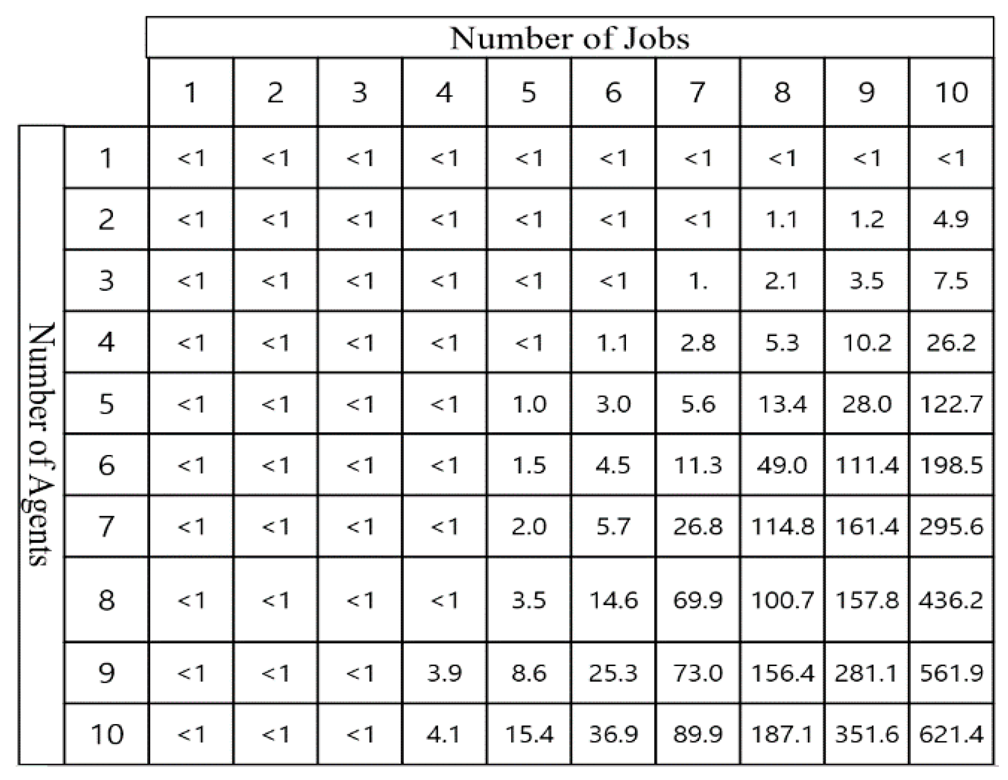
A total of 783,239 samples was generated for the raw data of the assignment to create the training dataset of the DNN. Figure 4 shows the average generation time of the PDDL solver for different numbers of agents and jobs. The generation time of the PDDL solver depends on the values of the parameters in each case and is calculated for up to 15 min to obtain samples of the dataset. If a sample that has elapsed for more than 15 min for generation is considered to be unsuccessful, it is excluded from the dataset.

Figure 4. Average generations time [s] for the combinations of the number of workers and jobs for the PDDL solver.

The PDDL method can be used to obtain results for the assignment problem. However, as the number of agents and jobs increases, the execution time of the PDDL solver increases rapidly. In a real-world application, it is necessary to solve the problem within a few seconds or less, depending on the required conditions, and a method that requires tens to hundreds of seconds to solve the problem is not practical.

In this study, a DNN was utilized to reduce the execution time of the search and to solve the assignment problem. The search time can be reduced to $O\left(1\right)$ by inferring that the DNN was trained using the dataset generated under the condition that the subproblem of the number of agents and jobs is within a maximum of 10.

4.2. Structures of the Training Dataset

The dataset for DNN training was created by preprocessing a large amount of raw data. The positions of the agents and jobs in the training dataset were scaled down to a size of 32 × 32. All agents and jobs were adjusted such that their positions did not overlap. The depth of the training dataset was 37 layers, and detailed information for each layer is shown in Table 1.

Table 1. Data Information for Each Layer in the Depth Direction of the Dataset.

Number of Depth Layers	Data Information
1	Worker’s unique ID $(\frac{\left(0~\left(m-1\right)\right)}{M}$)
2	Worker’s velocity ratio
3	Worker’s loading capacity ratio
4–13	Each worker’s sparse distance map between a worker and all jobs
14	Job’s unique ID $(\frac{\left(0~\left(n-1\right)\right)}{N}$) at start position
15–24	Each job’s sparse distance map between all workers and jobs from start position
25	Job’s unique ID $(\frac{\left(0~\left(n-1\right)\right)}{N}$) at target position
26–35	Each job’s sparse distance map between all workers and jobs from target position
36	All one value
37	All zero value

The target label data for multiclass classification is expressed as a two-dimensional matrix in which up to ten agents and ten jobs are matched, and labels are arranged in a one-dimensional array by concatenating each row of the matrix in succession.

4.3. Architecture of the Deep Neural Network

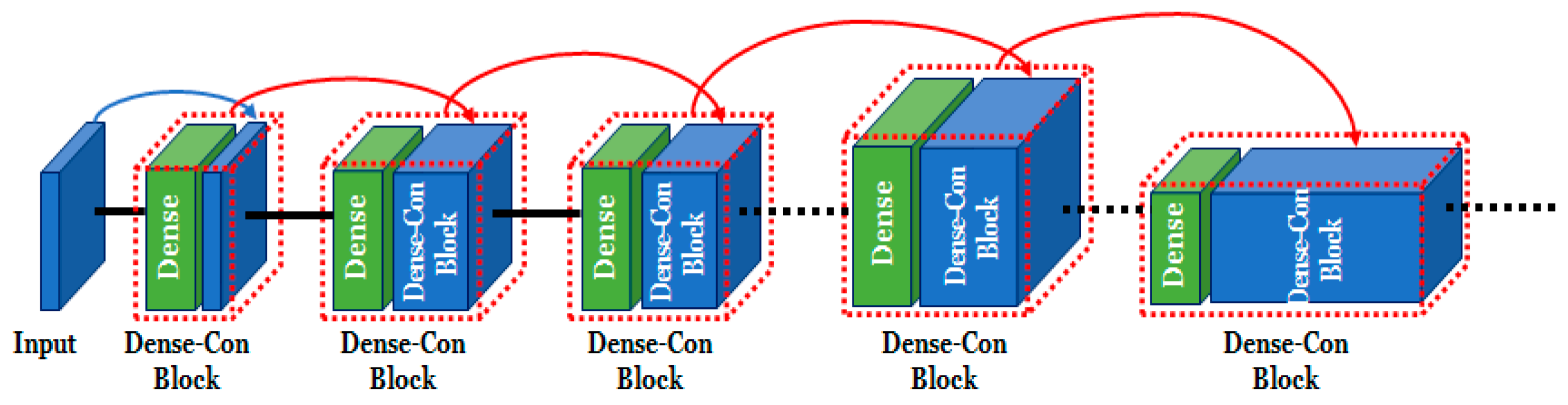
The proposed DNN is a dense-concatenate network (DeConNet) wherein the output of the previous dense layer is concatenated to the current layer and is connected to the input of the next layer. Its network structure is shown in Figure 5. The advantage of this network structure is that more layers can be stacked as the effect of the gradient vanishing problem is reduced. Deeper layers enable the neural network model to comprehend and elucidate complex domain contexts.

Figure 5. Network structure of nested block connection using the previous dense-concatenate block output as the input.

The architecture described in Table 2 utilizes the idea of DenseNet [32], which continuously connects the gradient calculated in the upper layer to the lower layer and is known to improve the vanishing gradient problem and feature propagation.

Table 2. DeConNet architecture for MDCOVRPPD dataset.

Layers	Layer Size (Output Shape)
Input	$\left(16\times 16\times 37\right)$
Dense-concatenate Block 1	$concatenat{e}_i {\left(\left[\begin{array}{c}Dense\left(74\right)\\ concatenat{e}_{i-1}\end{array}\right]\right)}_{i=1\dots 10}$
	$\left(16\times 16\times \left(74i+37\right)\right)$
Dense-concatenate Block 2	$concatenat{e}_i {\left(\left[\begin{array}{c}Dense\left(111\right)\\ concatenat{e}_{i-1}\end{array}\right]\right)}_{i=1\dots 10}$
	$\left(16\times 16\times \left(111i+777\right)\right)$
Dense-concatenate Block 3	$concatenat{e}_i {\left(\left[\begin{array}{c}Dense\left(148\right)\\ concatenat{e}_{i-1}\end{array}\right]\right)}_{i=1\dots 10}$
	$\left(16\times 16\times \left(148i+1887\right)\right)$
Dense-concatenate Block 4	$concatenat{e}_i {\left(\left[\begin{array}{c}Dense\left(111\right)\\ concatenat{e}_{i-1}\end{array}\right]\right)}_{i=1\dots 10}$
	$\left(16\times 16\times \left(111i+3367\right)\right)$
Dense-concatenate Block 5	$concatenat{e}_i {\left(\left[\begin{array}{c}Dense\left(74\right)\\ concatenat{e}_{i-1}\end{array}\right]\right)}_{i=1\dots 10}$
	$\left(16\times 16\times \left(74i+4477\right)\right)$
Dense-concatenate Block 6	$concatenat{e}_i {\left(\left[\begin{array}{c}Dense\left(37\right)\\ concatenat{e}_{i-1}\end{array}\right]\right)}_{i=1\dots 20}$
	$\left(16\times 16\times \left(37i+5217\right)\right)$
Dense-concatenate Block 7	$concatenat{e}_i {\left(\left[\begin{array}{c}Dense\left(18\right)\\ concatenat{e}_{i-1}\end{array}\right]\right)}_{i=1\dots 10}$
	$\left(16\times 16\times \left(18i+5957\right)\right)$
Dense Block	$\left(16\times 16\times 100\right)$
Classification Layer	$Flatten$
	$110D fully connected, softmax or sigmoid$

4.4. Training the Deep Neural Network

To train the DNN, each sample in the dataset was augmented by mixing the rotation for different directions, in addition to vertical and horizontal inversion. The number of augmented data was approximately 6,264,000 samples, which was eight times that of the original dataset.

Figure 6 shows the loss and accuracy of the epoch in the training and validation of the DNN. Given that the number of epochs was approximately 100 K, the loss decreased and the accuracy increased rapidly.

Figure 6. Loss and accuracy of training and validation for the deep neural network.

5. Experimental Results

5.1. Test Dataset of DNN

In the test dataset used to evaluate the performance of the DNN, test samples were generated for all cases within the maximum number of agents and jobs of 10, and the total number of samples was approximately 67,430. Table 3 lists the ground cost values for the test dataset. Table 3a represents the maximum (worst) and minimum (best) average travel times of the agent when all jobs are assigned to one agent. The left column of Table 3b is the sum of the average travel times of all agents when jobs are assigned to multiple agents. The right column of Table 3b shows the bottleneck of the average travel time of the agent, which was the longest when all agents started at the same time and completed their assigned jobs. Table 3c shows the average travel time reduction ratio when several agents divide and perform multiple jobs versus when one agent executes all jobs.

Table 3. Ground cost value of the test dataset.

Number of $\mathbf{Agents}\left(\mathit{j}\right)$ and $\mathbf{Jobs}\left(\mathit{k}\right)$		Cost (Average Travel Time [s])
		An Agent Does All the Work (a)		Multi-Agent Does Their Work (b)		Average Travel Time Reduction Ratio (c)
$\mathit{j}$	$\mathit{k}$	$\mathit{W}\mathit{o}\mathit{r}\mathit{s}\mathit{t}$	$\mathit{B}\mathit{e}\mathit{s}\mathit{t}$	$\mathit{S}\mathit{u}\mathit{m}$	$\mathit{B}\mathit{o}\mathit{t}\mathit{t}\mathit{l}\mathit{e}\mathit{n}\mathit{e}\mathit{c}\mathit{k}$	$\mathit{S}/\mathit{B}\mathit{e}\mathit{s}\mathit{t}$	$\mathit{B}/\mathit{B}\mathit{e}\mathit{s}\mathit{t}$
1	1	14.7	14.7	14.7	14.7	1.00	1.00
1	10	131.6	131.6	61.2	61.2	0.47	0.47
3	3	49.2	30.0	36.7	10.9	1.22	0.36
3	10	103.9	61.3	78.4	16.0	1.28	0.26
5	5	79.8	39.4	53.9	8.3	1.37	0.21
5	10	107.2	58.7	86.2	8.9	1.47	0.15
8	5	80.8	38.3	55.7	7.5	1.45	0.20
8	8	109.4	51.7	81.1	6.6	1.57	0.13
8	10	110.4	58.1	93.1	6.3	1.60	0.11
9	5	82.3	38.6	56.7	7.5	1.47	0.19
9	10	111.6	58.5	94.2	5.9	1.61	0.10
10	3	52.6	27.6	36.8	8.6	1.33	0.31
10	5	83.4	38.5	56.0	6.9	1.45	0.18
10	10	111.1	57.3	94.4	5.5	1.65	0.10

5.2. Inference Result of DNN

The hardware specifications used in the experiment for inference were a ASUS GL504G laptop with an Intel^® Core™ i7-8750H CPU and an NVIDIA GeForce RTX2070 GPU. Table 4 shows the results of comparing the ground cost of the test dataset to the prediction cost of the DNN. The left column of Table 4a is the sum of the average travel times of all the agents for the assignment of the PDDL solver in the test dataset. The right column of Table 4a shows the agent’s bottleneck of the longest average travel time when all agents started simultaneously and completed all jobs. Table 4b shows the sum and bottleneck of the average travel time of all agents for the assignment result based on the predictions of the DNN. Table 4c presents the reduction ratio of the average travel time for the assignment based on the DNN prediction or PDDL solver calculation.

Table 4. Result of comparing the ground cost of the test dataset with the prediction cost of the DeConNet.

Number of $\mathbf{Agents}\left(\mathit{j}\right)$ and $\mathbf{Jobs}\left(\mathit{k}\right)$		Cost (Average Travel Time [s])
		Ground Cost in the Test Dataset (a)		Prediction Cost of the DeConNet (b)		Average Travel Time Reduction Ratio (c)
$\mathit{j}$	$\mathit{k}$	${\mathit{G}}_{\mathit{S}}$	${\mathit{G}}_{\mathit{B}}$	${\mathit{P}}_{\mathit{S}}$	${\mathit{P}}_{\mathit{B}}$	${\mathit{P}}_{\mathit{S}}/{\mathit{G}}_{\mathit{S}}$	${\mathit{P}}_{\mathit{B}}/{\mathit{G}}_{\mathit{B}}$
1	1	14.7	14.7	14.7	14.7	1.00	1.00
1	10	61.2	61.2	61.2	61.2	1.00	1.00
3	3	36.7	10.9	36.6	12.0	1.00	1.10
3	10	78.4	16.0	79.7	17.2	1.02	1.09
5	5	53.9	8.3	54.3	8.9	1.01	1.07
5	10	86.2	8.9	85.7	9.7	0.99	1.09
8	5	55.7	7.5	55.3	7.8	0.99	1.03
8	8	81.1	6.6	79.9	6.9	0.98	1.04
8	10	93.1	6.3	91.8	6.8	0.99	1.08
9	5	56.7	7.5	56.2	7.6	0.99	1.01
9	10	94.2	5.9	94.0	6.4	0.99	1.10
10	3	36.8	8.6	36.7	9.1	0.99	1.04
10	5	56.0	6.9	55.9	7.5	1.00	1.08
10	10	94.4	5.5	93.6	6.1	0.99	1.13

As a result of the assignment between multiple agents and multiple jobs by inference of the DNN, the average travel time increased by a maximum of 13% in the case of a bottleneck compared with the ground truth. The result of the DNN inference is sometimes better than the cost value of the ground truth in the case of the sum of the average travel times, indicating that the PDDL solver’s job assignment was not optimal globally.

Table 5 shows the inference computation time for the DNN, which has a time complexity of $O\left(1\right)$ because it requires an average of approximately 20 ms of constant time, regardless of the number of agents and jobs.

Table 5. Comparison of the execution time [s] of the ground cost to the prediction time of the DeConNet.

Number of $\mathbf{Agents}\left(\mathit{j}\right)$ and $\mathbf{Jobs}\left(\mathit{k}\right)$		Time (Algorithm Running Time [s])
		PDDL Solver (OPTIC) (a)	DeConNet (b)	Runtime Reduction Ratio (c)
$\mathit{j}$	$\mathit{k}$	${\mathit{T}}_{\mathit{G}}$	${\mathit{T}}_{\mathit{P}}$	${\mathit{T}}_{\mathit{P}}/{\mathit{T}}_{\mathit{G}}$
3	10	$7.48\times {10}^0$	$2.59\times {10}^{-2}$	$3.46\times {10}^{-3}$
5	10	$1.23\times {10}^2$	$2.50\times {10}^{-2}$	$2.03\times {10}^{-4}$
8	5	$3.49\times {10}^0$	$1.41\times {10}^{-2}$	$4.04\times {10}^{-3}$
8	8	$1.01\times {10}^2$	$1.52\times {10}^{-2}$	$1.50\times {10}^{-4}$
8	10	$4.36\times {10}^2$	$2.08\times {10}^{-2}$	$4.77\times {10}^{-5}$
9	5	$8.56\times {10}^0$	$2.10\times {10}^{-2}$	$2.45\times {10}^{-5}$
9	10	$5.62\times {10}^2$	$2.48\times {10}^{-2}$	$2.45\times {10}^{-3}$
10	5	$1.54\times {10}^1$	$1.40\times {10}^{-2}$	$9.09\times {10}^{-4}$
10	10	$6.21\times {10}^2$	$2.49\times {10}^{-2}$	$4.01\times {10}^{-5}$

6. Conclusions and Future Work

In this study, we developed a deep neural network to solve the job assignment problem between multiple agents and multiple jobs for a multi-agent system within a constant time.

To create a training dataset for the deep neural network, the PDDL domain describes the environment defined by various parameters for agents and jobs; the PDDL problem is described by varying the values of the parameters; and finally, the PDDL solver generates the assignment problem result for each case.

Our test results showed that the job assignment based on the inference of the deep neural network increased by up to 13% compared with the results of the PDDL solver in the case of a bottleneck. The proposed DNN method had a constant execution time (approximately 20 ms), whereas that of the algorithm used for the PDDL solver or the metaheuristic method in other studies increased rapidly according to the number of agents and jobs, and other parameters.

In future work, it will be necessary to reduce the size of the network and improve the deep neural network to solve the assignment problem. This includes the use of extended parameters to better represent real-world situations. We also intend to implement a deep neural network that predicts the order of execution of multiple jobs assigned to each agent in order to help agents perform their tasks.

References

- Dantzig, G.B.; Ramser, J.H. The Truck Dispatching Problem. Manag. Sci. 1959, 6, 80–91. [Google Scholar] [CrossRef]
- Gasque, D.; Munari, P. Metaheuristic, models and software for the heterogeneous fleet pickup and delivery problem with split loads. J. Comput. Sci. 2022, 59, 101549. [Google Scholar] [CrossRef]
- Martinovic, G.; Aleksi, I.; Baumgartner, A. Single-Commodity Vehicle Routing Problem with Pickup and Delivery Service. Math. Probl. Eng. 2008, 2008, 697981. [Google Scholar] [CrossRef] [Green Version]
- Alesiani, F.; Ermis, G.; Gkiotsalitis, K. Constrained Clustering for the Capacitated Vehicle Routing Problem (CC-CVRP). Int. J. Appl. Artif. Intell. 2022, 36, 1–25. [Google Scholar] [CrossRef]
- Torres, F.; Gendreau, M.; Rei, W. Crowdshipping: An Open VRP Variant with Stochastic Destinations. Transp. Res. Part C Emerg. Technol. 2022, 140, 103677. [Google Scholar] [CrossRef]
- Ramos, T.R.P.; Gomes, M.I.; Barbosa-Póvoa, A.P. A New Matheuristic Approach for the Multi-depot Vehicle Routing Problem with Inter-depot Routes. OR Spektrum 2020, 42, 75–110. [Google Scholar] [CrossRef]
- Shen, L.; Tao, F.; Wang, S. Multi-Depot Open Vehicle Routing Problem with Time Windows Based on Carbon Trading. Int. J. Environ. Res. Public Health. 2018, 15, 2025. [Google Scholar] [CrossRef] [Green Version]
- Wassan, N.; Nagy, G. Vehicle Routing Problem with Deliveries and Pickups: Modelling Issues and Meta-heuristics Solution Approaches. Int. J. Transp. 2014, 2, 95–110. [Google Scholar] [CrossRef]
- Shi, Y.; Lv, L.; Hu, F.; Han, Q. A Heuristic Solution Method for Multi-depot Vehicle Routing-Based Waste Collection Problems. Appl. Sci. 2020, 10, 2403. [Google Scholar] [CrossRef] [Green Version]
- Sitek, P.; Wikarek, J. Capacitated Vehicle Routing Problem with Pick-Up and Alternative Delivery (CVRPPAD): Model and Implementation Using Hybrid Approach. Ann. Oper. Res. 2017, 273, 257–277. [Google Scholar] [CrossRef] [Green Version]
- Panos, M.; Pardalos, D.; Graham, R.L. Handbook of Combinatorial Optimization; Springer: Berlin/Heidelberg, Germany, 2013; ISBN 978-1-4419-7996-4. [Google Scholar]
- Montoya-Torres, J.R.; Franco, J.L.; Isaza, S.N.; Jimenez, H.A.F.; Herazo-Padilla, N. A literature review on the vehicle routing problem with multiple depots. Comput. Ind. Eng. 2015, 79, 115–129. [Google Scholar] [CrossRef]
- Kumar, S.N.; Panneerselvam, R. A Survey on the Vehicle Routing Problem and Its Variants. Intell. Inf. Manag. 2012, 4, 66–74. [Google Scholar] [CrossRef] [Green Version]
- Braekers, K.; Ramaekers, K.; Van Nieuwenhuyse, I. The Vehicle Routing Problem: State of the Art Classification and Review. Comput. Ind. Eng. 2016, 99, 300–313. [Google Scholar] [CrossRef]
- Toth, P.; Vigo, D. The Vehicle Routing Problem. Monographs on Discrete Mathematics and Applications; Society for Industrial and Applied Mathematics: Philadelphia, PA, USA, 2002; Volume 9, ISBN 0-89871-579-2. [Google Scholar]
- Ngo, T.S.; Jaafar, J.; Aziz, I.A.; Aftab, M.U.; Nguyen, H.G.; Bui, N.A. Metaheuristic Algorithms Based on Compromise Programming for the Multi-objective Urban Shipment Problem. Entropy 2022, 24, 388. [Google Scholar] [CrossRef] [PubMed]
- Xiao, H. Algorithm of Transportation Vehicle Optimization in Logistics Distribution Management. In Lecture Notes on Data Engineering and Communications Technologies; Springer: Berlin/Heidelberg, Germany, 2022; Volume 125, pp. 861–865. [Google Scholar] [CrossRef]
- Li, J.; Fang, Y.; Tang, N. A Cluster-Based Optimization Framework for Vehicle Routing Problem with Workload Balance. Comput. Ind. Eng. 2022, 169, 108221. [Google Scholar] [CrossRef]
- Pasha, J.; Nwodu, A.L.; Fathollahi-Fard, A.M.; Tian, G.; Li, Z.; Wang, H.; Dulebenets, M.A. Exact and Metaheuristic Algorithms for the Vehicle Routing Problem with a Factory-in-a-Box in Multi-objective Settings. Adv. Eng. Inform. 2022, 52, 101623. [Google Scholar] [CrossRef]
- Kyriakakis, N.A.; Sevastopoulos, I.; Marinaki, M.; Marinakis, Y. A hybrid Tabu search–Variable neighborhood descent algorithm for the cumulative capacitated vehicle routing problem with time windows in humanitarian applications. Comput. Ind. Eng. 2021, 164, 107868. [Google Scholar] [CrossRef]
- Son, N.; Jaafar, J.; Aziz, I.; Anh, B. A Compromise Programming for Multi-Objective Task Assignment Problem. Computers 2021, 10, 15. [Google Scholar] [CrossRef]
- Moscato, P.; Cotta, C. A Gentle Introduction to Memetic Algorithms. In Handbook of Metaheuristics; Glover, F., Kochenberger, G.A., Eds.; Springer: Boston, MA, USA, 2010; Volume 57, pp. 105–144. [Google Scholar] [CrossRef]
- Accorsi, L.; Lodi, A.; Vigo, D. Guidelines for the Computational Testing of Machine Learning Approaches to Vehicle Routing Problems. Oper. Res. Lett. 2022, 50, 229–234. [Google Scholar] [CrossRef]
- Bylander, T. The Computational Complexity of Propositional STRIPS Planning. Artif. Intell. 1994, 69, 165–204. [Google Scholar] [CrossRef]
- Fox, M.; Long, D. PDDL2.1: An Extension to PDDL for Expressing Temporal Planning Domains. J. Artif. Intell. Res. 2003, 20, 61–124. [Google Scholar] [CrossRef]
- Agerberg, G. Solving the Vehicle Routing Problem: Using Search-Based Methods and PDDL. Master’s Thesis, Uppsala University, Uppsala, Sweden, 2013; p. 71. [Google Scholar]
- Cheng, W.; Gao, Y. Using PDDL to Solve Vehicle Routing Problems. Lecture Notes in Computer Science. In Proceedings of the 8th International Conference on Intelligent Information Processing (IIP), Oxford, UK, 28–30 August 2014; pp. 207–215. [Google Scholar] [CrossRef]
- Allard, T.; Gretton, C.; Haslum, P. A TIL-Relaxed Heuristic for Planning with Time Windows. In Proceedings of the International Conference on Automated Planning and Scheduling, Delft, The Netherlands, 24–29 June 2018; Volume 28, pp. 2–10. [Google Scholar]
- Sirui, L.; Zhongxia, Y.; Cathy, W. Learning to Delegate for Large-Scale Vehicle Routing. arXiv 2021, arXiv:2107.04139. [Google Scholar] [CrossRef]
- Lee, M.; Xiong, Y.; Yu, G.; Li, G.Y. Deep Neural Networks for Linear Sum Assignment Problems. IEEE Wirel. Commun. Lett. 2018, 7, 962–965. [Google Scholar] [CrossRef]
- Benton, J.; Coles, A.; Coles, A. Temporal Planning with Preferences and Time-Dependent Continuous Costs. In Proceedings of the Twenty-Second International Conference on Automated Planning and Scheduling, São Paulo, Brazil, 25–29 June 2012; Volume 22, pp. 2–10. [Google Scholar]
- Huang, G.; Liu, Z.; Laurens, V.D.M.; Weinberger, K.Q. Densely Connected Convolutional Networks. In Proceedings of the IEEE Conference on Computer Vision and Pattern Recognition, Honolulu, HI, USA, 21–26 July 2017. [Google Scholar] [CrossRef] [Green Version]