Sequence Planner: A Framework for Control of Intelligent Automation Systems

Abstract

This paper presents a framework that tackles the challenges met in the development of automation systems featuring collaborative robotics and other machines that have some degree of autonomy. These machines rely on online algorithms for both sensing and acting in order to achieve a very high level of flexibility. To take advantage of these new machines and algorithms, control systems must also be increasingly flexible. In this paper, we present a framework for control of this new class of intelligent automation systems called Sequence Planner (SP), which helps with control of both traditional automation equipment and machines with autonomy. To aid the complex task of developing automation control solutions, SP relies on supporting algorithms for control logic synthesis and online planning. SP has been implemented with plug-in support for the Robot Operating System (ROS) and applied to an industrial demonstrator. We present our findings on how SP performed as a control system for this demonstrator, where we show that it is an adequate approach to implement automation for a highly flexible single station system. As a standardized way of automating such systems is missing, we hope that our contribution will provide a foundation for how to develop intelligent automation systems.

1. Introduction

Automated production systems are currently undergoing a transformation. Manually programmed operations are in the process of being replaced by online algorithms that are more dynamic and can react to a changing environment [1,2].

Current trends in automation include introducing more collaborative robots [3] and automated guided vehicles (AGVs), which, together with human operators, can provide more dynamic automation solutions. However, in order to provide a fully dynamic automation solution, the automation system needs to be able to both anticipate and react to what the surrounding environment as well as each subsystem will do next. In this work, this type of system is denoted as an intelligent automation system. This means that online algorithms for vision and motion planning need to be part of the automation system. Online algorithms for computer perception and complex motion tasks, such as grasping, do not have a 100% success rate today (e.g., [4,5,6]), and because of this, the use of such algorithms naturally increases the expected number of unsuccessful operations. Failures need to be handled as a natural part of controlling the automation system. This adds complexity to the control system software since more situations need to be handled. New methods and tools will be required to handle this increased complexity while maintaining high standards in safety and reliability.

One challenge in developing this type of system is software integration. The Robot Operating System (ROS) [7] is a set of software libraries for integrating various hardware drivers and online algorithms. Integration is performed by communicating over a publish/subscribe protocol using standardized message types. Using the standardized message types allows for quick and easy integration of new algorithms and drivers.

In order to handle large distributed networks, ROS leverages the Data Distribution Service (DDS) [8] communication architecture. While it cannot handle true real-time communication [9], being built on top of DDS makes it possible to use in real-world industrial applications [10].

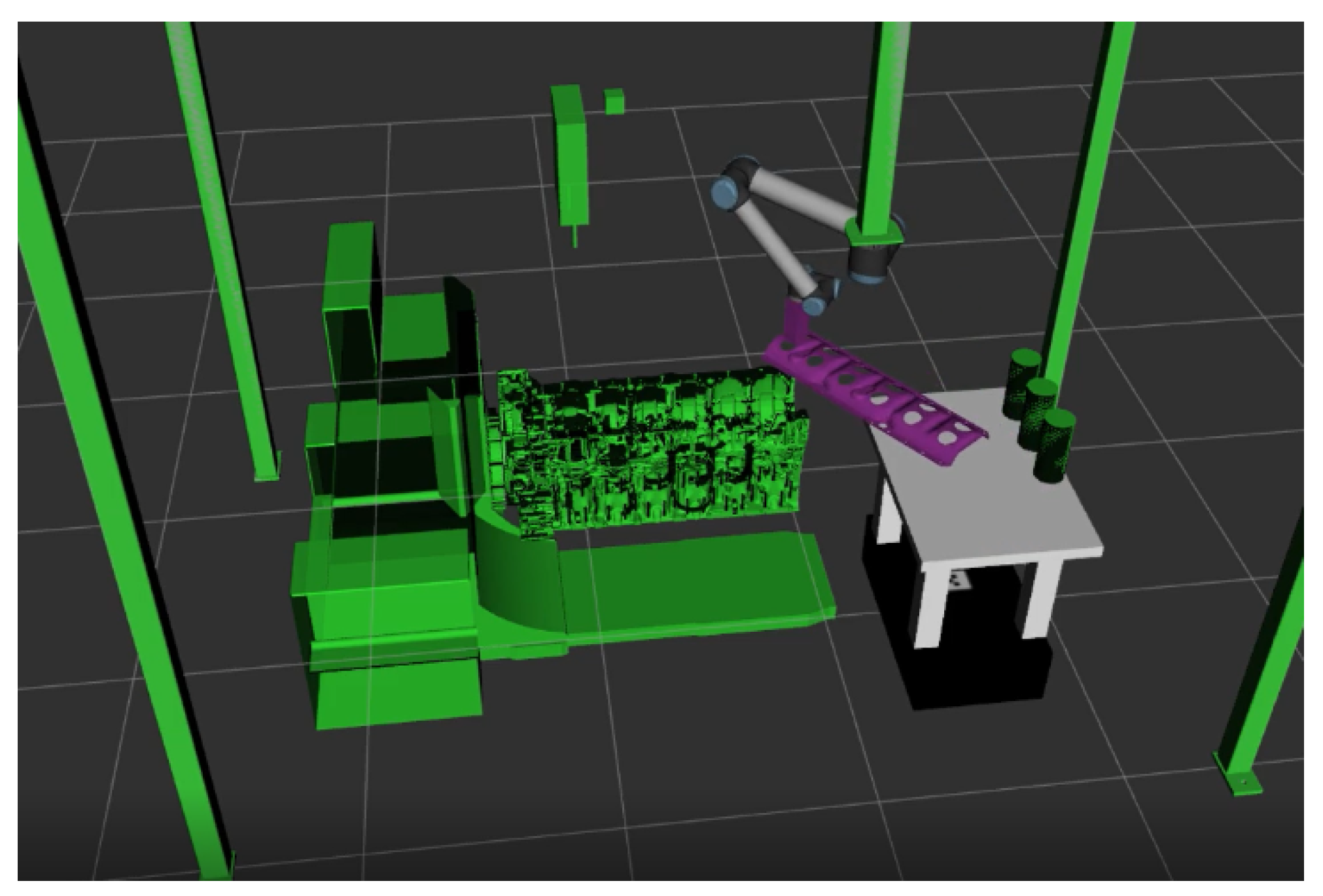
A simulated prototype of an industrial demonstrator, which will be described later in Section 3, is shown in Figure 1. The figure shows a simulation of a robot in the ROS vizualization tool RViz. Open source drivers for the robot can be connected to open source algorithms for robotics motion planning, for example MoveIt! [11], which in turn is built on top of the Open Motion Planning Library [12], which includes a variety of state-of-the-art motion planning algorithms. This highlights the composability of an open source software stack. As the open source libraries mature further, and with a solid communication layer (DDS), ROS is a good candidate for basing future automation systems on.

While ROS can give support with regards to integrating different software libraries and drivers, as well as provide a base layer for communication, challenges remain. One big challenge is the coordination of different devices, including robotic arms and AGVs, especially when erratic human behavior needs to be taken into account. In the literature, several frameworks have been proposed that aim to aid in the composition and execution of robot actions. One example is ROSPlan [13], which uses PDDL-based models for automated task planning as well as handling plan execution. Another is SkiROS [14], which is based on defining an ontology of skills. MaestROB [15] adds natural language processing and machine learning to teach robots new skills that are executed using ontology-based planning; CoSTAR [16] is based on Behavior Trees that are used to manually define complex behavior, combined with a novel way of defining computer perception pipelines; and eTaSL/eTC [17] defines a task-specification language based on constraints. Applications that use planning of robot skills have seen successful experimentation in industrial settings [18,19].

However, these systems have been mainly robot-oriented (in contrast to automation-oriented) and often focus on a single robot. None of them seem suitable for combining both high-level robotic tasks with more “traditional automation” tasks—low-level execution and state management of a variety of different devices. This paper presents a control framework for ROS that aims to aid in controlling multiple interdependent resources. The resources are modeled independently as components that include formal models of their behavior [20,21] and are controlled using a low-level planner. In order to ensure safe execution, constraints derived from safety specifications are added to restrict the planning system [22]. These constraints are designed to restrict the freedom of the planning system as little as possible. A high-level planner enables reactivity with regards to volatile system state and unpredictability of operators. An additional feature of SP is the natural way to handle restart and recovery from an error. Contrary to traditional automation solutions where restart can be quite tricky to manage, error recovery is now a part of the model in SP. This means that it is the planner’s task to automatically calculate an execution that will recover the system in a formally correct way [23].

1.1. Contribution

The proposed framework handles the increase in complexity brought by intelligent automation by off-loading difficult modeling tasks to control logic synthesis algorithms and the specifics of execution to an online planning system. This paper builds on the previous publications [10,20,22] and introduces new abstractions: operations and intentions, which enable hierarchical modeling and planning to make it easier to handle larger systems than in previous work.

We evaluate SP by applying it to an industrial demonstrator, where SP is used to control a wide variety of hardware as well as an extensive library of software including algorithms for real-time motion control. The experimental results of this application are presented. Previous works have described this application in the context of error handling [23]; however, this paper instead evaluates the general planning performance as well as describes in more detail how SP works.

1.2. Outline

Section 2 describes the proposed control framework. Section 3 describes an example application where the framework has been applied. Then, Section 4 contains experimental results from applying the framework to the application. Finally, Section 5 contains some concluding remarks and directions for future work.

2. The Sequence Planner Control Framework

The Sequence Planner (SP) control framework is based on goals. Goals define the states that it is desired for the automation system to be in. As an example, we can imagine that a certain part can be either unmounted or mounted. A goal for the automation system could then be that the part is mounted. In order for the automation system to reach this particular state, a sequence of actions needs to be performed depending on the state of the environment. We call this sequence of actions a plan. Due to the dynamic nature of intelligent automation systems, the environment may be uncertain, for example because there may be a human operator involved. As such, it must be possible to change plans to react to the changing environment. This is conducted in SP by continuously replanning to find a suitable plan.

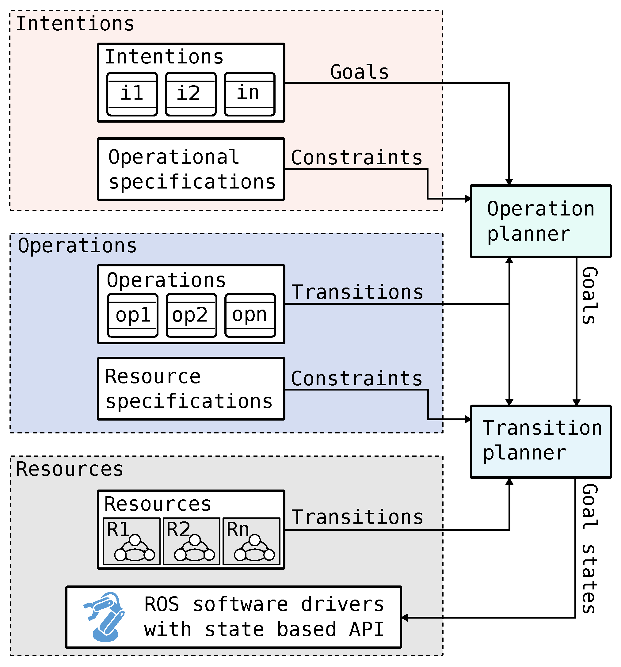
In order to have a responsive system, replanning needs to be fast. In SP, fast replanning is accomplished by dividing the work into two levels. Figure 2 shows an overview of the framework with the two planners to the right. The higher-level operation planner computes an abstract plan that the lower-level transition planner uses to compute detailed plans, which, when executed, distributes goal states to the resources that make up the automation system. The resources are intended to be reusable and are accompanied by a discrete behavior model that models how the resources can transition between their internal states, which allow them to be used directly with the planner. The composition of resources is performed via an abstraction called operation, which links an abstract planning model to detailed resource states. Additionally, resource specifications are added to ensure that the planner only takes safe routes to the goals. Intentions define the current goals that the operations should try to reach under operational specifications such as sequencing and priority choices.

2.1. Resources

Devices and software algorithms in the system are modeled as resources, which group their local state and discrete descriptions of the tasks they can perform. The resource state is encoded into variables of three kinds: measured state, goal state, and estimated state. The state of a resource corresponds to messages of specific types on the ROS network. These message types are generated from the definitions below.

SP models the resources using a formalism with finite domain variables, states that are unique valuations of the variables, and non-deterministic transitions between states. The following definitions are provided for clarification.

Definition 1.

A transition system (TS) is a tuple $\langle S,\to ,I\rangle$, where S is a set of states, $\to \subseteq S\times S$ is the transition relation, and $I\subseteq S$ is the nonempty set of initial states.

Definition 2.

A state $s\in S$ is a unique valuation of each variable in the system, e.g., $s=\langle v_1,v_2,\cdots ,v_n\rangle$.

Variables have finite discrete domains, i.e., Boolean or enumeration types.

The transition relation → defines the transitions that modify the system state:

Definition 3.

A transition t has a guard g, which is a Boolean function over a state, $g:S\to \{false,true\}$, and a set of action functions A where $a:S\to S$, which updates the valuations of the state variables in a state. We often write a transition as $g/A$ to save space.

Definition 4.

A resource i is defined as $r_i=\langle V_i^M,V_i^G,V_i^E,T_i^c,T_i^a,T_i^e\rangle$ where $V_i^M$ is a set of measured state variables, $V_i^C$ is a set of goal state variables, and $V_i^E$ is a set of estimated state variables. Variables are of finite domain. The set $V_i=V_i^M\cup V_i^G\cup V_i^E$ defines all state variables of a resource. The sets $T_i^c$ and $T_i^a$ define controlled and automatic transitions, respectively. $T_i^e$ is a set of effect transitions describing the possible consequences to $V_i^M$ of being in certain states.

$T_i^c$, $T_i^a$, and $T_i^e$ have the same formal semantics, but are separated due to their different uses:

Controlled transitions $T_i^c$ are taken when their guard condition is evaluated to be true, only if they are also activated by the planning system.

Automatic transitions $T_i^a$ are always taken when their guard condition is evaluated to be true, regardless of if there are any active plans or not. All automatic transitions are taken before any controlled transitions can be taken. This ensures that automatic transitions can never be delayed by the planner.

Effect transitions $T_i^e$ define how the measured state is updated, and as such, they are not used during control such as for the control transitions $T_i^c$ and $T_i^a$. They are important to keep track of, however, as they are needed for online planning and formal verification algorithms. They are also used to determine if the plan is correctly followed—if the expected effects do not occur, it can be due to an error.

Consider the case of a door with two binary sensors: one for detecting whether it is open, and one for detecting whether it is closed. The door can be opened and closed by the control system, but not moved to an arbitrary position. The measured state for this door resource would be two Boolean variables, closed: $c_{?}$ and opened: $o_{?}$ (to ease notation in the coming sections, we use a notation in which measured state variables are denoted with a subscript “?”, goal state variables are denoted with a subscript “!”, and estimated state variables are denoted with a hat—see

Table 1. Notation for the three different types of a resource state variable v.

$v_{?}$	measured state variables
$v_{!}$	goal state variables
$\widehat{v}$	estimated state variables

). To control the door, a goal state variable model is introduced: $g{s}_{!}\in \{closed,opened\}$.

A resource d modeling the door as a component can then be defined as $r_d=\langle \{c_{?},o_{?}\},$$\left\{gs\right\},Ø,\cdots \rangle$. Note that $V_d^e=Ø$. This is the ideal case because it means all local states of this resource can be measured. We will come back to the transitions of the resource model soon.

From $r_d$, with some additional metadata such as data types and topic names, ROS message definitions can be automatically generated. Listing 1 shows the generated message definitions for the door, which define the interface to the door node. It is also possible to generate a template for an ROS node that can be used to connect either directly to the sensors (e.g., reading I/O:s) or listen to some already existing node, in which case a translation may need to be performed (perhaps the door is already publishing sensor data on the network) [10].

Listing 1. ROS message definitions for messages on the topics from and to the door.

# ROS topic: /door/measured bool closed          # => $c_{?}$ # ROS topic: /door/goal bool close           # => $c_{!}$

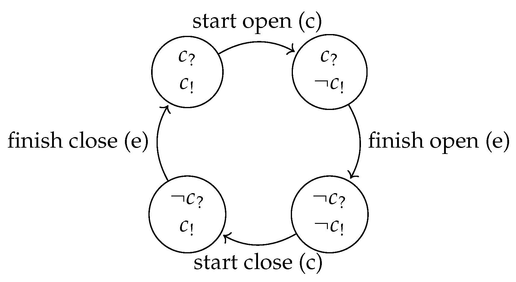
It is natural to define when to take certain actions in terms of what state a resource is currently in. To ease both modeling and online monitoring, resources can contain predicates over their state variables. These predicates can be used in the guard expressions of the transitions. For example, one such predicate could be $\mathit{doorIsClosing}:c_{!}\wedge \neg c_{?}$. Figure 3 shows the states and transitions of the resource that relate to opening the door, where $\mathit{doorIsClosing}$ is true in the bottom left state. The transitions have descriptive names which also denote their type: controlled transitions have an appended (c), automatic transitions have an appended (a), and effect transitions have an appended (e). There is no notion of an initial state—the planner is always called with the current state of the resources.

The resource and ability defined, combined with the corresponding ROS2 node(s), makes up a well isolated and reusable component. However, at this point, it cannot do anything useful other than being used for manual or open loop control. One also needs to be able to model interaction between resources, for example between the door resource and a lock resource. Interactions are modeled using operations and resource specifications.

2.2. Operations

In addition to the variables defined by the resources, another set of variables exists: decision variables. These define the state of the system in abstract terms for scheduling and planning which operations to execute. For example, a decision variable could be the abstract state of a particular resource, or the state of a product in the system. Sometimes decision variables can be directly measured by resources, in which case these measurements are copied into the decision variables, usually after undergoing some form of transformation (for example discretization). The resources and decision variables make up a global state transition system.

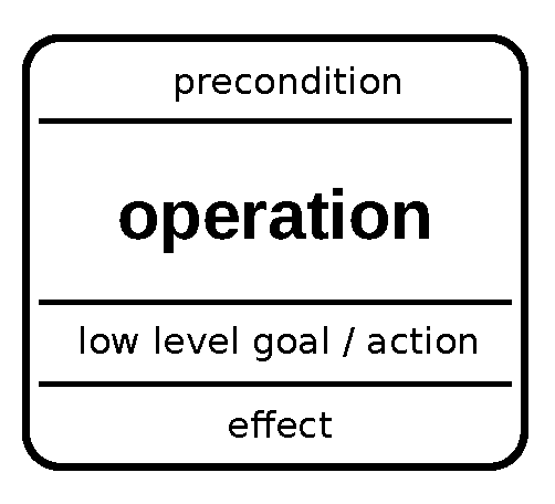
Definition 5.

An operation j is defined as $o_j=\langle p_j,e_j,g_j,a_j,s_j\rangle$, where $p_j$ is a precondition over the decision variables defining when the operation can start; $e_j$ is a set of actions completing the operation, which are actions that modify the decision variables; and $g_j$ is a goal predicate defined over the resource variables. $a_j$ is a set of actions for synchronizing the operation with the resource state. Finally, the operation has an associated state variable $s_j\in \{i,e,\mathit{error}\}$. Throughout the paper, operations are graphically depicted as in Figure 4.

When the precondition of an operation is satisfied, the operation can start. The effect actions are then evaluated against the current state, and the difference between the current state and the next state is converted into a predicate. This predicate becomes the post-condition of the operation; e.g., if the precondition is $x\ne y$ and the action is $x:=y$, then the post-condition (and thus its planning goal) becomes the valuation of y at the time of starting the operation.

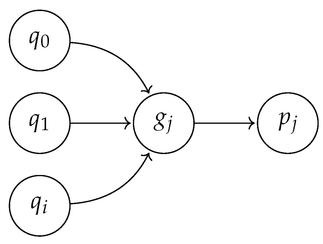
To enable the planning system to reach the goals of the operation j, an automatic transition from the low-level goal predicate of the operation ($g_j$) is added to the global TS. See Figure 5, where $q_0$, …, $q_i$ represent different states from which states in the set defined by $g_j$ can be reached, and $p_j$ is the set of states reachable from $g_j$ after taking the transition which updates the decision variables according to the effect $e_j$.

Encoding the operation effects as automatic transitions ensures that the effects will take place even if the goal state was reached without the planner. In other words, it means that if the resources are put into a state which satisfies $p_j$ for some operation $o_j$, the decision variables are updated automatically. This is especially useful after an error scenario, where there may not be a clear view of which operations should currently be active, but it is known which state the operator desires the system to be in, or when the system state is modified manually.

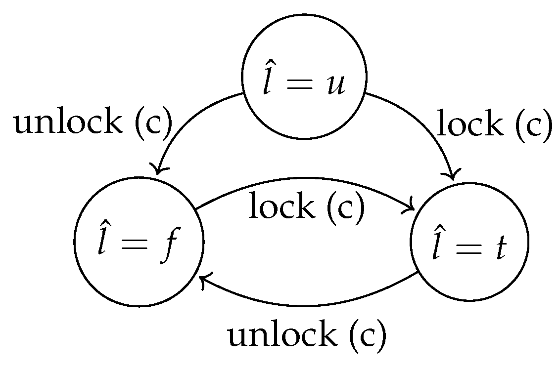
To exemplify operations, we now revisit the door example. Recall that we would like to add a locking mechanism to our door. Instead of going back and rewriting the door resource and generated node, we would like to compose the door with an existing “lock” resource. The lock has two goal variables, $l_{!}\in \{false,true\}$ and $u_{!}\in \{false,true\}$, requesting whether it should be locked or unlocked. The lock does not have a sensor, and therefore the state of it must be estimated. To keep track of whether it is locked or not, the resource includes an estimated state variable $\widehat{l}\in \{unknown,false,true\}$. The lock can be locked even though it is already locked, to put it in a known state, which also applies to unlocking. This means that we must encode events using our goal states.

The resource $lock$ defining the door can then be defined as $r_{\mathit{lock}}=\langle Ø,\{l_{!},u_{!}\},\left\{\widehat{l}\right\},\cdots \rangle$. Figure 6 shows the transition system of the lock resource.

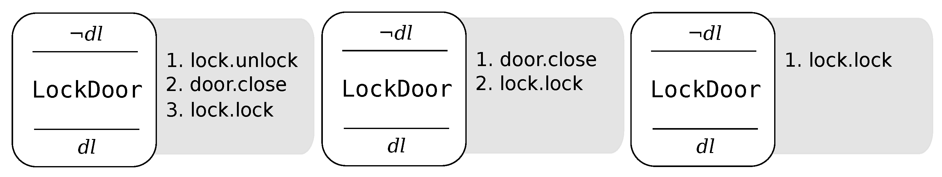
If it is important that the door is sometimes locked, a decision variable describing that the door is locked (in contrast to only the lock being locked) is introduced: $dl$ (“door locked”), together with an operation which locks it. As it does not make sense to lock the door while it is open, the operation LockDoor ($o_l$) defines $c_{?}\wedge \widehat{l}$ as its goal state ($g_l$). That is, it uses state from both the door resource and the lock resource. The precondition of the operation ($p_l$) is $\neg dl$, the action is $dl:=true$.

Essentially, it is the automatic transition created, which updates the decision variable, that models the interaction between the two resources. It enables the planner to try to reach $dl$, which means that it has to visit the state $c_{?}\wedge \widehat{l}$. Additionally, the automatic transition ensures that if the door is closed and locked manually, the decision variable in the control system will be updated automatically.

Depending on the starting state, executing the operation will have different consequences. Figure 7 shows three possible (well-behaved) plans that can arise from executing the operation.

With the decision variable and the operation defined, it is now possible to track whether the door is locked, which requires the door and the lock to coordinate their actions (closing and locking). However, nothing prevents the planner from locking the lock and then closing the door, or opening the door while the lock is locked—something which is obviously “bad” behavior.

2.3. Resource Specifications

Formal specifications can be used to ensure that the resources can never do something “bad”. In order to be able to work with individual resources, as well as isolating the complexities that arise from their different interactions, modeling can rely on using global specifications. By keeping specifications as part of the model, there are fewer points of change, which makes for faster and less error-prone development compared to changing the predicates manually, a time-consuming and difficult task.

SP has no notion of implicit dynamics or memory, i.e., all memory states need to be explicitly modeled using the estimated variables. Often, the decision variables are enough to act as memory, however (they are treated the same as estimated variables). This means that the state of the system is solely defined in terms of the valuations of the variables in the system. In order to constrain the system, it is desired to eliminate all states that violate certain specifications.

In SP, specifications can be entered as invariant formulas over the system variables that make up the system state. Due to the way automatic transitions (which should always be taken) and effect transitions (which can happen non-deterministically) are defined, these invariant formulas need to be expanded to cover a larger set of states, due to the fact that the system can move uncontrollably between these states.

To do this, the negation of an invariant formula (i.e., the forbidden states) is extended into larger sets of states using symbolic backwards reachability analysis [22]. After expanding these regions, the symbolic representation is minimized using the espresso heuristic [24] and converted back to a propositional formula that is provided to the planner.

In the door example, we can specify that it should not be possible for the door to close when the lock is locked. If we use the named predicate $doorIsClosing$ defined earlier, this can be expressed as $\mathit{doorIsClosing}\Rightarrow \widehat{l}=false$, i.e., whenever the door is closing, the lock is (known to be) unlocked.

In this case, the result of such a specification will be that the system cannot execute $g{s}_{!}:=opened$ when $\widehat{l}\ne unlocked$ and cannot execute $l_{!}:=true$ when $g{s}_{!}\ne opened$.

Similarly, but more simply, a specification can ensure that it should not be possible to open the door when it is locked, mirroring the physical reality. In this case, the use of synthesis is clearly more of a modeling convenience since adding an “is unlocked” term to the enabled predicate is easy. However, having it in a specification keeps the interaction between resources in one place. A specification that forbids the door to be closed when $\widehat{l}=\mathrm{unknown}$ can be added in the same way. Modeling this uncertainty is conducted so that the system can operate to some degree even in the unknown state, which ensures that a restart after errors can be performed using the control system rather than following a fixed procedure for putting things in a known state.

2.4. Intentions

While the operations define interactions between resources via goal states and how they relate to the decision variables, intentions model how to make the system do something useful. As an example, we will be using the door with the lock to secure a room where two autonomous roaming robots charge their batteries. The position of the robots is modeled as decision variables $r_1\in outside,inside$ and $r_2\in outside,inside$, where inside refers to being inside the room with the door. To define a task that locks both AGVs in the room, an intention is used. An intention defines a goal over the decision variables. In this case, we define a goal g as: $g:=(dl\wedge r_1=inside\wedge r_2=inside)$.

Definition 6.

The intention k is defined as $i_k=\langle p_k,g_k,{\varphi }_k,a_k,s_k\rangle$, where $p_k$ is a predicate over (all) the variables in the system, defining when the intention starts (automatically); $g_k$ is a goal predicate defined over the decision variables; ${\varphi }_k$ is an optional LTL formula over the decision variables; $a_k$ is a set of actions that can update (all) variables in the system, which are applied when the intention finishes; and $s_k\in \{i,e,f\}$ is the state of the intention.

The intentions are free to change the state of the system ($a_k$) in arbitrary ways upon finishing, in order to be able to create hard-coded state machines for deciding when each intention should be active. As the intentions exist on a high abstraction level, these state machines are generally quite small and can be managed manually. The planning problem can be constrained using the LTL formula ${\varphi }_k$, which allows for specifying, for example, sequencing constraints. We will come back to LTL in Section 2.6.

Now, we would like to “wire up” the goal g we defined above to a button that calls the AGVs home. The button is a resource that has a measured state variable $b_{?}$. We create an intention i: $\langle s_i=i\wedge b_{?},g,{\varphi }_i,s_i:=i,i\rangle$, i.e., it has a precondition that triggers on itself being in the initial state and the button being pressed, g is the goal predicate, it has an LTL formula ${\varphi }_i$ (defined later), it has a single action which resets the intention upon finishing (to be able to activate it immediately again), and its state is initially i.

It is easy to see how another operation for opening the door could be written, together with a similar intention, which could be wired up to a button $b_{2?}$. What happens when both buttons are pressed simultaneously? Since it is not possible to reach both locked and open at the same time, one of the intentions will fail. This is easily avoided by adding guard expressions to the intentions that forbids them from activating at the same time.

The operation abstraction eliminates the need for reasoning about individual resource states. Details about whether the lock is initially locked or not, or whether the door is opened or closed or somewhere in between, can be kept out of the programming of the intentions. These details are instead off-loaded to the planning system.

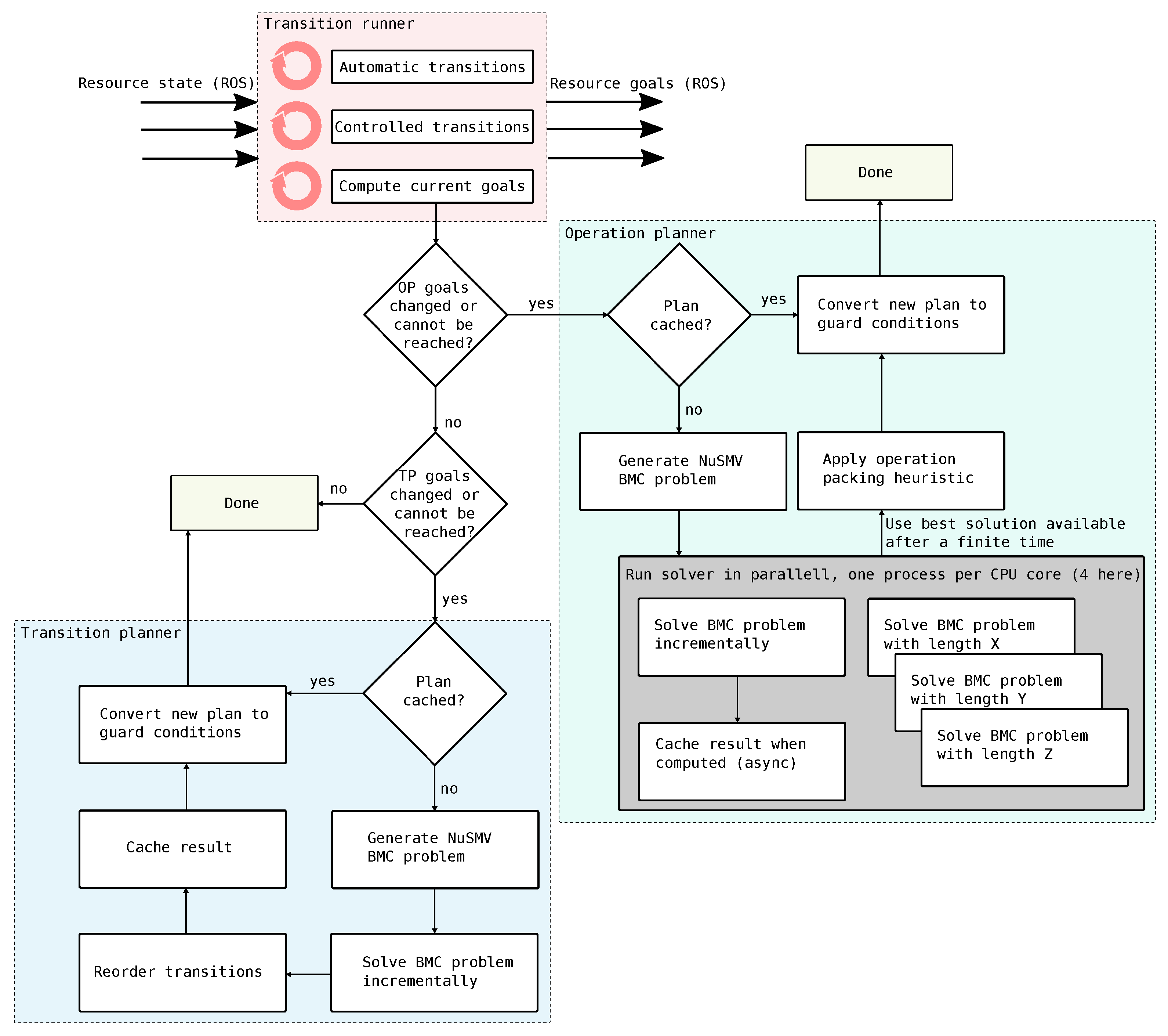
2.5. Transition Runner

The transition runner (top part in Figure 8) keeps track of the current state of all resource states, decision variables, operations, and intentions. The transition runner continuously applies transitions which update the system state, reacting to any changes to the incoming state from the ROS nodes on the network. The transition runner operates solely in terms of taking any available transitions. This includes both controlled transitions and automatic transitions.

A transition can be taken when its guard expression is evaluated to be true in the current state, after which the action functions update the state. In order to distribute the goals to the resources, the state variables that relate to such goals are published on appropriate ROS topics.

Every time a new plan is calculated, controlled transitions are supplemented with additional guard expressions, which define the order of execution and the external state changes that the transition has to wait for. As the planner will never allow any forbidden states to be reached, operations and intentions that are active based on their state can sometimes randomly be changed, in order to abort an active intention or a running operation.

2.6. Operation Planner

The operation planner (right part of Figure 8) is used to find a sequence of operations that should reach the goals of any currently active intentions. Currently, the planning engine in SP is based on nuXmv [25], which is a model checker rather than a classical planner. A model checker can prove temporal properties about a model by exploring the state space defined by a set of initial states and a set of transitions [26]. Temporal properties can be written in different ways, for example Computation Tree Logic (CTL) or Linear Temporal Logic (LTL) [27], which are both extensions to propositional logic. Such extensions include operators for expressing properties on past or future states. LTL has operators for the next state (operator X) that some formula should always (G) hold, that it should eventually hold (F), and that one formula should hold until another one does (U). For example, the formula $\mathbf{G}$ $(x\to \mathbf{X}y)$ expresses that it is always the case that x implies y in the next state. In bounded model checking (BMC) [28], a reduction to Boolean satisfiability is performed with an upper bound on the number of transitions from the initial state that can be included. This allows for fast Boolean satisfiability (SAT) solvers to be used to find counterexamples.

By letting the model checker try to prove that a future (desired) state is not reachable, a counterexample, if found, can be used as a plan. This allows for the use of LTL specification that needs to be true for the duration of the plan.

Consider the example of locking the door to secure the AGVs again. If both AGVs are outside the room, we want to give priority to $r_1$ to enter the room first. However, if $r_2$ is already in the room, it should not be forced to move out of the room just so $r_1$ can enter first. We can express this operational specification using LTL in terms of the decision variables: $r_2=outside\wedge$$\mathbf{X}{r}_2=inside\Rightarrow r_1=inside$. The specification models with $r_2$ transitioning from outside to inside imply that $r_1$ is already inside.

As seen in Figure 8, the transition runner continuously checks whether the goals of the currently executing intentions are reachable. This is performed by simulating the current plan against the current state. If the goals cannot be reached, or if the goals have changed, a new operation plan needs to be computed. A cache of plans is checked to see if this particular plan has already been computed before. If no plan is cached, a new BMC problem is generated, where the initial state is the current state of the system.

A generated BMC problem and a minimal length counterexample for the example with the door and two robots can be seen in Listing 2. It includes the decision variables $dl,r_1,r_2$, and a transition relation which is generated from the operation definitions based on $p_j$ and $e_j$ for operation j. The IVAR:s keep track of which transitions are taken in each step. An initial state is provided based on the current state of the automation system. Lastly, the goal is expressed as an LTL specification, where the LTL operator U is used to specify that the formula ${\varphi }_i$ should hold until the goal is reached. The counterexample is a trace of which transitions were taken in order to violate the LTL specification (recall that the BMC problem is inverted).

Listing 2. To the left: generated BMC problem for the problem of the door and the two robots. To the right: counterexample which can be used as a plan.

MODULE main VAR   dl : boolean;   r1 : {outside,inside};   r2 : {outside,inside}; IVAR   lock_door : boolean;   r1_go_in : boolean;   r2_go_in : boolean; TRANS lock_door & !dl & next(dl) = TRUE &         next(r1) = r1 & next(r2) = r2 | r1_go_in & !dl & r1 = outside & next(r1) = inside &        next(dl) = dl & next(r2) = r2 | r2_go_in & !dl & r2 = outside & next(r2) = inside &        next(dl) = dl & next(r1) = r1; ASSIGN   init(dl) := FALSE;   init(r1) := outside;   init(r2) := outside; LTLSPEC ! ( ((r2 = outside & X(r2 = inside)) -> r1 = inside) U             (dl & r1 = inside & r2 = inside) );

Trace Type: Counterexample   -> State: 1.1 <-     dl = FALSE     r1 = outside     r2 = outside   -> Input: 1.2 <-     lock_door = FALSE     r1_go_in = TRUE     r2_go_in = FALSE   -> State: 1.2 <-     r1 = inside   -> Input: 1.3 <-     r1_go_in = FALSE     r2_go_in = TRUE   -> State: 1.3 <-     r2 = inside   -> Input: 1.4 <-     lock_door = TRUE     r2_go_in = FALSE   -> State: 1.4 <-     dl = TRUE

The standard BMC formulation solves SAT instances of increasing length, corresponding to steps into the future from the initial state. This means that it automatically produces minimal length counterexamples. However, the SAT solver is usually much faster at finding a satisfying solution than determining that the previous plan lengths in unsatisfiable. Therefor we apply a variant of the strategy suggested in [29], where the underlying SAT problem is solved with varying lengths simultaneously (one per CPU-core). This makes finding an initial plan a lot quicker, but it has the downside that the plan can contain unnecessary steps. To mitigate this, a heuristic is applied to keep searching for a little longer after a satisfying solution has been found, in order to minimize the number of unnecessary steps in the plan. Incrementally finding the minimal length counterexample is performed asynchronously as a background task and added to the planning cache once computation has finished.

A downside to using a BMC solver as the planning engine is that the counterexample trace has a fixed sequential execution ordering—it is a totally ordered plan rather than a partially ordered plan [30]. A partial order plan can execute some steps in parallel, where the ordering of actions does not change to final outcome. To enable multiple operations to start in parallel, ordering among independent operations is removed a as a post-processing step in SP. Operations are considered independent if their set of used variables (i.e., the set of all variables used in the goal predicates, preconditions, and effect actions) is disjoint.

2.7. Transition Planner

In a similar way as the operation planner computes plans that should reach the goals of the currently active intentions, the transition planner computes plans that should reach the goal states of the executing operations. The transition planner continuously compares its current plan to the system state to see if the plan is still valid. Whenever the goals change, or if they can no longer be reached with the current plan, a new plan is computed. An overview of the transition planner is shown in the bottom part of Figure 8.

A BMC problem is generated that includes the automatic, controlled, and effect transitions. The initial state is set at the current state of all resources, estimated states as well as all decision variables. Further, the BMC problem is constrained by any invariant formulas (see Section 2.3. Since the operations and decision variables define a hierarchy, the abstraction needs to be ordered monotonic [31]. This can be handled by forbidding the transition planner from changing any decision variable that is not in the currently active goal. This prevents the transition planner from completing operations that the operation planner did not intend to complete.

The resource models only contain information about which transitions can be taken from certain states and which are expected to be taken from certain states. Thus, there is no inherent notion of a “task” that can be considered independent from other tasks. For this reason, it is not possible to compute a partially ordered plan as is done with the operation planner. Instead, a strategy which starts activities eagerly is implemented as a post-processing step. In this strategy, transitions are reordered using a simple algorithm which, if possible, “bubbles” any transitions that are not effects up to the top of the plan. We do this with the assumption that controllable transitions usually start things, while effect transitions usually end things. For example, consider the case of two independent resources which can perform task a and task b. To start the tasks, an IO is set high $a_{!}:=true$ and $b_{!}:=true$ for the respective tasks. The tasks are deemed finished when sensors read $a_{?}=true$ and $b_{?}=true$, respectively.

Table 2. Transition reordering.

step 1	controllable	$a_{!}$	step 1	controllable	$a_{!}$
step 2	effect	$a_{?}$	step 2	controllable	$b_{!}$
step 3	controllable	$b_{!}$	step 3	effect	$a_{?}$
step 4	effect	$b_{?}$	step 4	effect	$b_{?}$

shows the original plan to the left and the plan after “bubbling up” the transitions that are not effects to the right. The original plan will have unnecessary waiting before task b is started.

The algorithm used to “bubble up” transitions works in the following way: if a transition is not an effect, it is iteratively swapped with the previous transition as long as the goal can still be reached by following the totally ordered plan exactly. This is conducted for all transitions in the plan, starting at the top and working down to the bottom, swapping order whenever possible.

2.8. Non-Determinism

Because the resources are modeled as non-deterministic transition systems, it is possible that there are multiple effects from a single state. This is useful to model alternatives. However, the operation planner does not branch on these but will always “choose” the best possible outcome whenever there are multiple possible outcomes of an operation. While it is possible to compute plans that take branching into account, this increases complexity as the planning problem essentially becomes a controller synthesis problem [32]. In SP, the strategy is to let the planner decide on the “correct” outcome, and instead replan upon encountering an unexpected result.

In order to also capture the non-determinism in the decision variables, “variants” of operations are allowed, which are copies of the same operation but with different actions and goal states. When an operation that has a variant is executing, the goal of the transition planner is set to the disjunction of the operation variants’ goals. For example, consider a sensor (${\mathit{sens}}_{?}$) that scans the color of a product, determining that the product is either red or green. An operation “scan” could exist in two variants, one with a goal predicate ${\mathit{sens}}_{?}=\mathit{red}$ and an outcome that a decision variable is assigned “red” and one with a goal predicate ${\mathit{sens}}_{?}=\mathit{red}$ and the outcome that a decision variable is assigned “green”. The goal for the transition planner would then be ${\mathit{sens}}_{?}=\mathit{red}\vee {\mathit{sens}}_{?}=\mathit{green}$. When ${\mathit{sens}}_{?}$ receives one of the values, the decision variable is updated accordingly. This may trigger replanning of the operation planner if the “correct” outcome was not achieved.

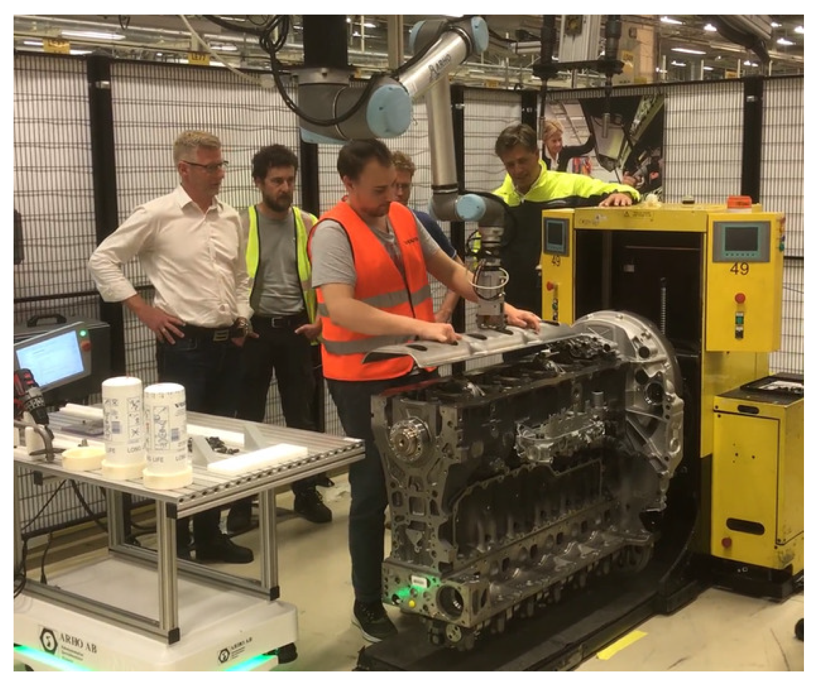
3. Application to an Industrial Demonstrator

To validate the design, the described framework has been applied to an industrial demonstrator. This case has been described in previous publications [10,20,22], but an overview is given here. The demonstrator is located in a manufacturing facility for truck engines, and it concerns the assembly of several components onto the engine block. The challenge is in the way that the operator and a collaborative robot have to perform operations. Namely, the operations can be executed either by the robot, the human, or in a collaborative fashion. An extensive software library, motion planning and vision algorithms, as well as a wide variety of hardware are used to achieve this. A photo of the assembly system can be seen in Figure 9, where an operator and a collaborative robot place a cover plate onto the diesel engine.

To tackle different tasks in the system, it was necessary to dedicate eight computers. These computers run software for the physical resources of the system such as the Universal Robots collaborative robot, the Mir100 autonomous mobile platform, the end-effector docking station, the nutrunner lifting system, the RFID reader and camera system, as well as the nutrunner tool itself, which can be operated both by the operator and the robot.

When developing this industrial demonstrator, the main focus was on the robustness aspects of performing a collaborative engine assembly using machines and operators. Even if important aspects such as operator safety, performance, and real-time constraints were considered in this work, they were not the main focus while developing this demonstrator. Such important aspects will be addressed in future work, especially the safety of human operators.

3.1. Human Operator

Some tasks are performed in a coactive fashion, such as lifting a heavy metal plate onto the diesel engine assisted by the robot, but the human operator should be free to perform tasks independently of the machines in the system. This means that human behavior takes precedence—the machines should aid the operator and not be a hindrance. The operator is free to perform its individual tasks without adhering to fixed sequences, if it is not required to assemble the product correctly.

This requires constant measurements of what the operator is performing, for example by tracking the position of the human and using smart tools that can sense when the operator successfully performs tasks. It is the flexibility provided by the planner, or more specifically, the act of replanning, that enables the operator to act freely. As soon as the automation system realizes (through continuous forward simulation) that the current goal cannot be reached—perhaps because the operator has changed something—a new plan is computed. Additionally, the ability to cancel active intentions (which in turn cancels operations) means that the automation system can be given new goals in reaction to a changing environment.

One of the tasks that should be performed at the assembly station is moving an engine cover plate, called a “ladder frame”, from an autonomous kitting robot onto the engine and bolting it down. This involves several resources: the UR10 robot, the connector, an end-effector for lifting the plate, the nutrunner, and a human operator. The UR10 and the nutrunner are hanging from the ceiling, and the UR10 can attach itself to the nutrunner to guide it to the pairs of bolts on the ladder fame.

3.2. Resources

The developed system contains a number of different resources, and they are distributed over several different computers. All communication between the computers is performed via ROS over DDS. Resources model both physical machines and software services, e.g., drivers for the UR10 robot, connectors, nutrunners, tools, a motion planning service based on MoveIt! [11], and a UI for the operator. Since the resources are modeled independently, they can easily be reused.

3.3. Operations

The automation system has been modeled with 30 different operations, which involve localization of equipment and products, moving robots, and performing assembly using the smart tools. Decision variables keep track of whether the position of parts is known, who is holding the tools, and the state of the products. These can change on external input, for example, if a human operator is using a smart tool in manual mode.

4. Results

In this section, we describe our findings of applying SP to control the intelligent automation system described in Section 3. We are interested to know how often new plans are computed and how quickly this can happen.

4.1. Planning Performance

The planners effectively define a hierarchy. This means that there exists a trade-off between the “length” of the chosen operations and the number of operations. For instance, having a decision variable that models the knowledge about which tools are held by the robot is not necessary. This is because the transition planner will decide and carry out the necessary resource transitions when the time comes to perform bolting.

However, to ensure reactivity, it is necessary that both planners react quickly. This is especially true for the transition planner, which contains all the details and as such a huge number of possible paths, of which we also want the “shortest”—it is crucial not to try to compute too-long plans.

Another aspect comes when we want to perform optimization instead of planning over the operations. If the operations have a time associated with them (which can be different based on the state of the resources when the operation is started), knowledge about whether a tool change is needed to perform the operation can be of crucial importance.

We provide some preliminary planning benchmarks on the example system. The transition planning model includes 6 resources and has 84 transitions (of which 30 are auto transitions coming from operations), 58 specifications, and $1.02434\times {10}^{22}$ reachable states. The operation planning model is orders of magnitudes smaller, with $1.61248\times {10}^9$ reachable states and 30 transitions modeling the operations.

The transition and operation planning times, ordered by plan length, are shown in Figure 10. The plans were computed on a consumer-grade laptop computer, and every single computed plan is represented by a cross. As it can be seen from Figure 10, the transitions planner can comfortably plan 15–20 steps ahead, while keeping the system responsiveness under 1 s. For the most part, though, the system behaves nominally. This means that even if SP can handle great flexibility, there are few occasions where replanning is needed.

4.2. Rate of Plan Computation

The plots in Figure 11 show the rate at which new plans are computed given that the system starts with empty planning caches. The data were recorded in a simulation of the system during four assembly cycles (one cycle takes 210 s, depending on how much the operator does in advance or interferes). In the 16 min data collection period, the automation system produced 160 unique transition plans, averaging one plan per 6 s, and 35 unique operation plans, averaging one plan per 27 s. The system is left alone in the first half of the chart, which leads to steadily increasing cache hits for both planners once the same sequences are being played out again. In the second half, a human operator starts “interfering” by completing assembly tasks using a smart tool as well as being in the way, which leads to an increase in the rate of new plans being computed. While this paper does not go into detail about how SP performs error handling, error situations are handled by replanning, which is also a factor when it comes to how quickly the number of plans grow.

4.3. Plan Complexity

As can be seen in Figure 11a, transition plans are generally between 7 to 18 steps long. Commonly, plans are comprised of several pairs of control actions coupled with expected effects, for example giving a command and waiting until the action has finished before taking the next step in the plan. This means there are around three to nine different actions in each transition plan (sometimes less when resources expose intermediate states).

By running the system without the operation packing heuristic, only one operation is run at a time, allowing us to count the number of resources involved in reaching each operation goal. We find that the number of resources included in an operation plan is between two and four, with most of the operations using only two resources. It is interesting to note that there is no operation which only uses a single resource. The large number of operations which utilize two resources are the ones which use the robot and a tool, for example, to tighten bolts and oil filters, but there are also situations where a resource that is not actively involved in an operation needs to move to a certain state during completion due to a specification. The operations that involve more resources include, for example, calling a robot motion planning service, and setting IOs for the connector attached to the robot.

5. Conclusions

This paper introduced Sequence Planner (SP) as a framework to model and control intelligent automation systems. The control framework has been implemented with support for ROS and applied to an industrial demonstrator.

The focus in SP is to assume control of the internal state machines of the individual resources. This allows the complex task of coordinating many resources to be handled by the transition planner, even though there are complex interdependencies between resources. Resources can be made highly reusable by applying the proposed combination of resource specifications and operations as the main modeling concept.

Achieving a good result, however, requires that the modeling task be performed to a high standard. Modeling errors will be found and used as loop-holes by the transition planner. The requirements of a well-modeled system indicate that there need to be guarantees about what can and cannot happen. Writing, testing, and then trusting the written specifications make formal verification and virtual validation crucial tools during development.

We have found that the operations as defined in SP are a natural way to define a hierachical model, in contrast to PPDL-based planning systems such as ROSPlan, where Hierarchical Task Networks (HTNs) [33] need to be defined. However, due to the differences in modeling language, no direct comparison has yet been made between the two difference systems.

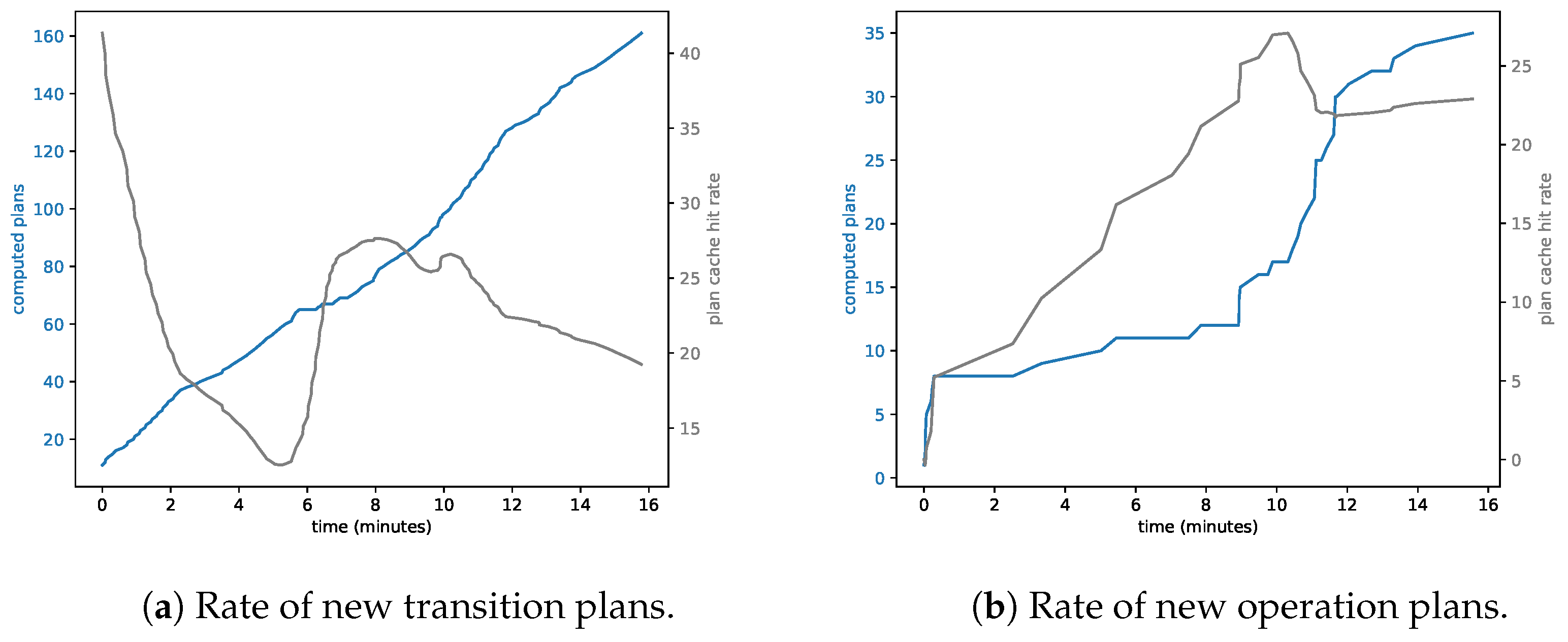
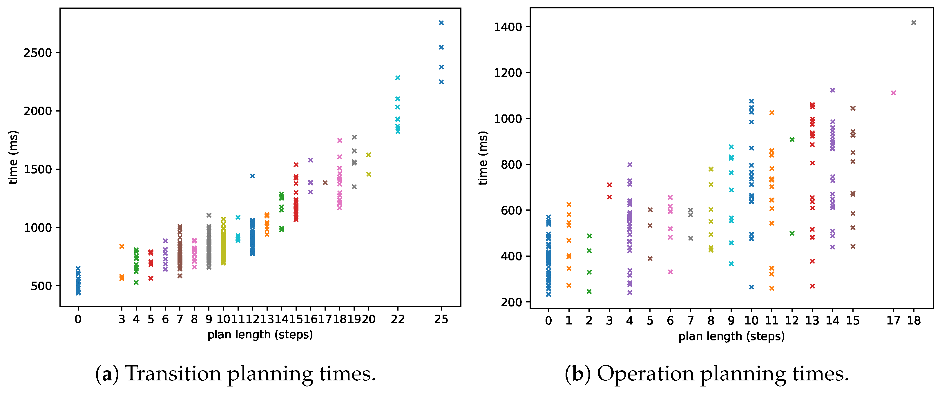
Naturally, a system that relies on formal methods and online planning has an upper limit to the complexity of the model. State space explosion is an issue, both for verification and for efficient planning. As we can observe in Section 4, planning times go up to around 1–2 s for the longer plans. This implies that the proposed framework cannot handle much larger systems than presented in Section 3. However, as long as the complexity of a single station is not too high, the framework should be applicable. Additionally, new state-of-the-art planners and model checkers can be utilized to increase the raw performance.

Future work will involve learning a distribution of the duration of the operations (which naturally fluctuate depending on the state of the resources), which can be used by the operation planner to find time-optimal plans. Additionally, an investigation should be made on how the operation planner can take into account non-deterministic effects. This could reduce the need for replanning and allow more time to instead be spent computing a high-quality plan.

Sequence Planner is open source software and can be found at http://github.com/sequenceplanner/sp (accessed on 24 May 2022).