Abstract
Worldwide, lung cancer is one of the most common causes of cancer-related death. Detected by computer tomography, it is usually removed through thoracoscopic surgery. During the surgery the lung collapses requiring some strategies to track or localize the new position of the lesion. This is particularly challenging in the case of minimally invasive surgeries when mechanical palpation is not possible. Here we undertake a preliminary study with numerical analysis of an ultra-wideband (UWB) radio technology which can be employed directly during thoracoscopic surgery to localize deep solitary pulmonary nodules. This study was conducted through Finite Difference Time Domain (FDTD) simulations, where a spherical target mimicking a nodule located between 1 and 6 cm of depth and an UWB pulse at several frequencies between 0.5 and 5 GHz was used for localization. This investigation quantifies the influence of several parameters, such frequency, lesion depth, and number of acquisitions, on the final confocal image used to locate a cancer in the lung tissue. We also provide extensive discussion on several artifacts that appear in the images. The results show that the cancer localization was possible at operational frequencies below 1 GHz and for deep nodules (>5 cm), while at lower depths and higher frequencies several artifacts hindered its detection.
1. Introduction
As of 2018, lung cancer is the most commonly diagnosed cancer with circa 12% of tumor cases worldwide [1,2]. Despite advances in therapy, the five-year survival rate is approximately 18% [3] and with 18.4% of the total, it is the leading cause of cancer-related death [1].
Solitary pulmonary nodules (SPNs) have a prevalence of 50% in lung cancer screening studies of high-risk smokers, which is becoming an increasing clinical problem [4,5]. They are usually detected incidentally by low-dose helical computed tomography (CT) and, as general rule, with high probability of malignancy, such as solid and subsolid SPNs, evidence of growth, and size larger than 8 mm, the lesion should be biopsied or surgically excised for diagnosis [4,6].
This is performed by video-assisted thoracoscopic surgery (VATS) when a nonsurgical biopsy is unavailable, not practical, or nondiagnostic. However, in the case of small, deep and solitary pulmonary nodules its localization is particularly challenging [7].
VATS falls in the group of minimally invasive procedures where the surgeon makes some small incisions in the skin and inserts several long and thin tubes into the patient body. At one end of the tubes there is either a miniaturized camera, called a laparoscope, or other laparoscopic instruments, such as dissecting forceps and scissors. A minimally invasive surgery has the advantage of a faster recovery and less postoperative pain because of the smaller incisions in the patient body.
Although the position of the lung nodule was known before surgery, due to the lung collapse at thorax opening, a new localization is necessary. However mechanical palpation is not possible during laparoscopic surgery [4] and different methodologies are used. The cancer can be marked by CT-guided operations which involve the insertion of a percutaneous needle through the chest wall toward the nodule or in its close proximity. The percutaneous needle is either used to insert a guidewire with a metal hook at the end or to inject a small quantity of methylene blue. The risks associated with these procedures can be pneumothorax, hemothorax, or pulmonary hemorrhage due to the needle insertion. Or in the case of the methylene blue, uncontrolled spillage of the dye over the complete site making the subsequent localization of the tumor impossible [8].
Alternatively, intraoperative imaging with ultrasonography, fluoroscopy, or molecular imaging devices are used [4]. Nevertheless, air pockets remain in the alveoli and bronchioles even when the lung is in a deflated state producing artifacts in the ultrasound image [9,10] and fluoroscopy and molecular imaging are unable to provide information of deep lesions [4]. Therefore an innovative methodology is sought to address the problem of localization of pulmonary lesions in operando conditions.
On the other hand, for breast cancer, which is the leading case of cancer-related death for women [2], microwave imaging is widely used. This technique employs non-ionizing radiation in the frequency range between 300 MHz and 30 GHz and therefore can develop images of the internal tissues of the human body with low health risk. The imaging is based on the backscattering of the electromagnetic waves given by dissimilarities in dielectric properties of different tissues. These properties are tabulated for a large variety of human tissues [11,12,13,14] and can be found online [15].
The backscattered signal (echo) is used to reconstruct the morphology of the medium through Confocal Microwave Imaging (CMI). The locations of any dielectric dissimilarity are inferred through synthetic focusing upon irradiation with an ultra-wideband (UWB) electromagnetic pulse from different physical positions.
Confocal microwave imaging has been under development for two decades in the detection of breast cancer [16,17,18]. While only in recent years researchers moved toward lung cancer [19,20]. One of the main challenges in lung cancer detection through microwave imaging is the large number of tissues the electromagnetic wave needs to travel through compared to breast cancer analysis. In fact the ultra-wideband pulse encounters several layers of skin, bones, and muscles before reaching the lung. Therefore we suggest illuminating the lung directly during VATS. This would greatly simplify the problem of multiple scattering given by several layers of different tissues. However, this approach is not free from adversities as lung tissue has high dielectric permittivity and conductivity. The latter strongly attenuates microwaves reducing their penetration depth, but on the other side, it also hinders backscattering and clutter from neighbor organs.
Compared to breast cancer, lung cancer has a relatively low difference in dielectric properties compared to the surrounding tissue. The difference in permittivity is between a factor of 1.2 to 3 times higher than the permittivity of the healthy lung tissue and a factor of 1.6 to 2 for the conductivity (values extrapolated from reference [21]). These factors are as high as 5.5 and 2 for the breast cancer permittivity and conductivity, instead [16]. This potentially produces lower contrast in the confocal images.
This contribution represents a preliminary analysis, performed by numerical simulations, of microwave imaging of lung cancer. This is the first work on the problem of localization of pulmonary lesions by microwave imaging during video-assisted thoracoscopic surgery. The final goal is to screen several parameters on the confocal imaging which will be used in future works to design a microwave transmitter/receiver for a laparoscopic instrument. The parameters investigated are the frequency of the ultra-wideband (UWB) signal, the depth of the lung nodule to localize, and the distribution of the antennas, as summarized in Table 1. The simulations were performed in such a way to mimic the direct illumination of a collapsed lung, but to keep the results as general as possible, a particular model for the transmitter/receiver antennas was not employed.

Table 1.
Parameters investigated.
2. Materials and Methods
Similarly to our previous work [22], a half-space composed of air at the top and a medium with the dielectric properties of a deflated lung at the bottom was simulated through 3D Finite Difference Time Domain (FDTD) using a recompiled version of gprMax version 3.1.5 [23,24] which allowed double precision calculations.
An FDTD solver was selected because it offers a straightforward implementation of the problem at hand. It also scales almost linearly with the problem size and it offers the possibility to create movies of the wave propagation which are important for understanding and troubleshooting. In particular gprMax was selected because it is open-source, easy to modify (we recompiled it for our purposes) and use, and geared for ground-penetrating problems which are very similar to microwave imaging of targets in biological tissues.
The FDTD solves the four Maxwell’s equations:
together with the constitutive relations:
in space on a staggered grid though the use of Yee cells [25] and electric- and magnetic-field quantities are computed at alternating time steps.
The Equations (1)–(4) are also known as Faraday’s law (Equation (1)), Ampère’s circuital law (Equation (2)), Gauss’s law (Equation (3)), and the nonexistence of a magnetic monopole (Equation (4)) [26]. They describe how the electric field E and the magnetic field H are interconnected through the electric displacement field D, the magnetic flux density B, their time derivative, the volumetric charge density , and the current density J which is comprised of the conductive current and the surface current .
In addition, the Equations (5)–(7) represent the constitutive relations. They link D, B, and to the local properties of the materials which form the computation domain. These properties are the dielectric permittivity , the magnetic permeability , which is usually taken as zero for biological materials, and the conductivity . In general, they are time-dependent, viz. frequency dependent, and Equations (5)–(7) are convolutional relations (note the convolution sign ∗). The dielectric permittivity and the conductivity for lung tissue (deflated lung taken from reference [15]) are reported in Figure 1 together with the wavelength and attenuation of the electromagnetic wave calculated for the lung tissue.
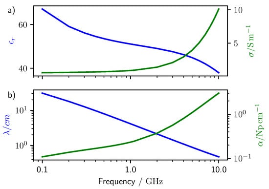
Figure 1.
Dielectric properties of lung tissue taken from the Tissue Properties Database [15]. (a) relative dielectric permittivity and conductance of lung tissue. (b) Wavelength and attenuation of a plane wave traveling through lung tissue (calculated from a).
A schematic of the half-space used for the computations is illustrated in Figure 2 together with one antenna distribution () on the top of the lung tissue which is displayed in violet. Lung tissue properties were taken from the Tissue Properties Database [15] (considering deflated lung as material reference). Permittivity and conductivity were changed according to the central frequency of the electromagnetic pulse, however, no dispersive properties were actually implemented in the simulation, that is for every simulation the dielectric properties of the materials were taken as frequency independent. The excitation pulse used was the derivative of a 1 V amplitude Gaussian function (gaussiandot in gprMax). Ten central frequencies between 0.5 and 5 GHz were used as excitations and additional simulations were performed at 1 GHz to investigate extra parameters (see Supplementary Information SI).
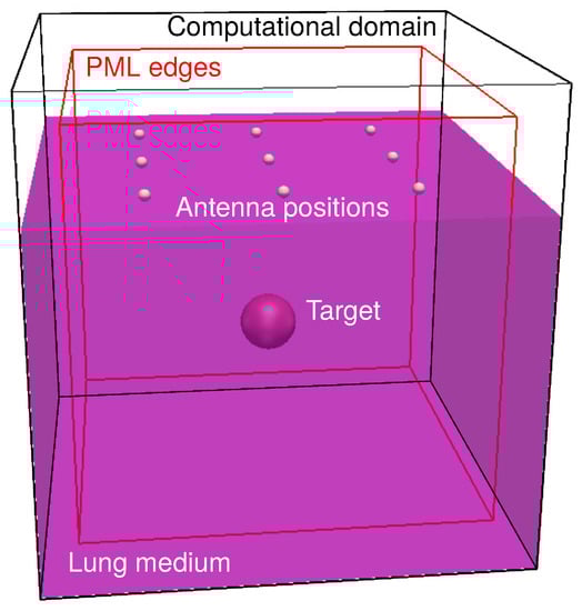
Figure 2.
Schematic of the 3D computational domain. The violet parallelogram represents the lung medium. Inside the lung medium, the target is present (red sphere). On top of the lung medium a antenna distribution is shown. A simulation was performed at each of these positions. The edge of the Perfectly Matched Layers (PMLs) are shown in red.
In this frequency range the wavelength of the electromagnetic wave in the lung tissue has a dimension comparable to that of a solitary pulmonary nodule of 8 mm, which is the threshold size for diagnosis (see Figure 1b). Note that higher frequencies would provide higher spatial resolution, but their attenuation in the lung tissue increases quickly (see Figure 1b).
Ten-cells wide perfectly matched layers (PML) as highlighted in red in Figure 2 were used to truncate the computation in all the directions and the discretization was either 12 divisions per wavelength at the central frequency or 1 mm according to the smallest size.
A pulmonary nodule was simulated by a spherical target with 0.5 cm of radius placed in the middle of the lung, as it is recommended that nodules larger than 8 mm should be biopsied or surgically excised for diagnosis [4,6]. Six target depths between one and six centimeters were investigated. The permittivity and conductivity of the cancer were taken from the work of Wang et al. [21] where it was found that at 100 MHz, lung cancer had permittivity three times and conductivity two times larger than that of the lung medium.
A monostatic antenna assembly was made of a voltage source with 50 Ohm impedance and z polarization and a simple receiver. The receiver recorded the value of the electric field at the position of the voltage source. This configuration is less effective than a real physical model of an antenna, but it allows us to study the backscattered signals independently of the antenna characteristics such as bandwidth and gain directivity. Note that, for most of the frequencies selected, the antenna would be receiving signals from within its near field, that is at a distance lower or comparable with the wavelength of the electromagnetic wave employed. Only at the higher frequencies or larger distances, the antenna operates in its far-field (see Figure 1b).
The position of the antenna was changed according to a regular grid of size , , and as shown in Figure 2. A simulation was run for every antenna position resulting in nine simulations for the grid, 16 for the , and 25 for the . The antennas were spaced according to one wavelength of the electromagnetic wave in the lung medium. Any object as antenna and nodule target were at least thirty cells away from the end of the computation domain. The target was always located exactly under the center of the antenna grid. This represents the best configuration. Changing the alignment between the antenna grid and the target could create more realistic results, but it would also introduce additional degrees of freedom in the pool of simulations, which is not necessary as preliminary analysis.
This approach was designed to mimic a series of real measurements, where either an array of antennas is positioned at the surface of the lung or a single antenna is moved at several positions on the lung surface. In the first case one single measurement is taken at every one of the antenna positions as, for example, when a physical switch would connect it to the transceiver apparatus. In the second case the same antenna would be used to perform more measurements at different locations. The main advantage of an antenna array would be a precise and known distance between the antennas, as these are embedded in the array, and the possibility to work with several receivers at once. On the other side, a single antenna gives more flexibility in the positioning, but it also requires precise knowledge of the position where the recording was produced.
Only the z component of the electric field was used to reconstruct the confocal map through the Delay and Sum (DAS) algorithm [27]. Although several reconstruction algorithms exist, DAS is the simplest and still among the best performing ones [28]. In depth description of the DAS can be found elsewhere [16,22,28] and only a short description is presented here.
The DAS is composed of three parts. In the first part, the waveforms acquired by all the antennas are calibrated by subtracting their average. In fact, the averaged signal contains the reflection from the main tissues or objects which are in common to all the antennas, in this application the back-scattered signal deriving from the interaction between the air and the lung medium. The calibrated signals are then time aligned and integrated. This converts the back-scattered signals which were not removed by the calibration into bell-like peak shapes appearing at particular time delays. Radial attenuation was compensated by scaling the signals by the square of the distance. Every point of the half-space is then taken as synthetic focal point and the intensity I of the confocal map was reconstructed by [16,28]:
where is the calibrated waveform acquired at the antenna n and is the return time from the point to the antenna n. The return time was mapped into position considering the velocity of the electromagnetic wave in the medium. In this case the wave velocity was taken from the dielectric permittivity of the lung tissue at the central frequency of the electromagnetic excitation. Finally, the pixel intensity of the confocal maps was normalized to unity to facilitate the comparison.
3. Results and Discussions
Figure 3 shows the averaged waveform collected by the simulations performed with a 3 cm deep target at 1 GHz with a antenna grid. This is the average that was used to calibrate the waveforms. Since the receiver was located at exactly the same positions as the voltage source, all the recordings contained the main excitation pulse which is the only waveform appreciable in the figure. Every backscattering would be orders of magnitude smaller than this signal.
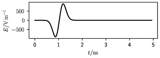
Figure 3.
Averaged waveform for a 3 cm deep target at 1 GHz central frequency and a antenna grid.
The calibrated waveforms for the simulation set of Figure 3 are reported in Figure 4. The waveforms are divided according to at which antenna they were recorded. A schematic of the antenna grid with the antenna position highlighted in gray is displayed at the top-right corner of every graph. Figure 4a shows the antenna in the corner positions, (b) and (c) those in symmetric position around the center, while (d) shows the calibrated waveform from the central antenna (see caption for details). It is noteworthy that the waveforms are not overlapping exactly inside the same group because of the finite space discretization level of the simulations. The triangle, the square, and circle in the middle of the graph indicate the expected time of some events. The triangle represents the central time of the excitation pulse.
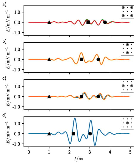
Figure 4.
Calibrated waveforms for a 3 cm deep target at 1 GHz central frequency and a antenna grid. The black triangle, square, and circle represent, in order from left to right, the middle time of the pulse excitation and the return time for the first and second interface of the target. (a) Waveforms for the corner antennas. (b) Waveforms for the top and bottom central antennas. (c) Waveforms for the left and right central antennas. (d) Waveform for the central antenna.
As it can be seen in Figure 3, at 1 ns the pulse had its zero-crossing middle point which can be used as reference time. In fact, this point is the same in all graphs of Figure 4. The second event, highlighted by a square, represents the return time of the echo from the first target interface. This time was calculated considering the average propagation speed of the electromagnetic wave in the homogeneous lung tissue and a straight line from the antennas to the target. This distance was the shortest for the central antenna (Figure 4d) and the longest for the antennas in the corner position (Figure 4a). In Figure 4b,c this return time is the same.
The last event, highlighted by a circle, corresponds to the return time of the echo coming from the second interface of the target, which is when the electromagnetic wave traveled past through the target in a straight line. In this case also the target material was considered to calculate the propagation speed.
It can be seen that the waveforms are relatively flat at the positions where Figure 3 has the maximum intensity, showing that the calibration procedure of the DAS algorithm indeed helps in enhancing the backscattered signals. In all graphs, there are some modulations at the time corresponding to the two target echoes (square and circle). These modulations are the strongest for Figure 4a and the weakest for (d). In fact, the antennas at the corners had the largest distance from the target, while that in the center the shortest. As it can be seen from Figure 1b, the lung tissue shows a non-negligible attenuation in all the frequency range which sums up with the standard attenuation experienced by a radial propagating wave.
Notice that there are other signals before the first target echo. These were produced by the bouncing of the electromagnetic wave in the half-space on top of the lung tissue. In fact, although PML boundaries were enforced, a fraction of the electromagnetic wave was not totally absorbed at the end of the computation domain and was reflected back toward the receiver. This is similar to a real case scenario where the materials surrounding or housing the antennas are not totally absorbing the radiation. These signals contribute to increasing the clutter, amount of undesired intensity, in the confocal maps. They are the strongest in Figure 4a). In this case, in fact, once hitting the target the electromagnetic pulse was, in addition, reflected vertically toward the lung–air interface which was considerably closer than the receiver. From there, since the dielectric permittivity of air is much smaller than that of the lung tissue, the wave could reach the receiver faster traveling through the air region than by simply remaining inside the lung tissue, producing some undesired signals.
For all the antenna positions, the intensity of the second echo (circle in Figure 4) was comparable with the intensity of the first one (square). This was a consequence of the small difference in dielectric properties between the lung tissue and the target material. In fact, the conductivity of this material, which affects the attenuation, was only a factor of two higher than the surrounding.
Passing to the confocal images, Figure 5 shows the confocal map for 0.6 GHz frequency, target depth of 6 cm, and an antenna distribution on top of the lung tissue following a grid. To better visualize the results, the confocal map is sliced parallelly to the x-plane (Figure 5a) and to the z-plane (Figure 5b), respectively. The slices intersect each other at the center of the target which is represented by a red circle. Note that the confocal images are oriented as Figure 2 with the antennas positioned on the top.
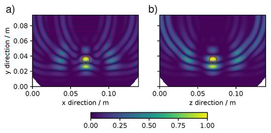
Figure 5.
Confocal map for a 6 cm deep target at 0.6 GHz with a antenna grid. (a) x-parallel slice and (b) z-parallel slice. Expected target position is indicated by a red circle.
In general, a good localization of the target requires that most of the pixel intensity should cluster at one position. In Figure 5 although there are clear and intense signals at the expected position of the nodule (red circle), the cluster at the target is not a continuous spot, but presents some modulations. This was not a novel phenomenon in confocal imaging, see for example reference [29], and in our case it can be reconnected with the findings of Figure 4 where some signals intensity was not only present at the return time expected for the target echos. However, despite the clustering, the target position could clearly be inferred although not with high accuracy.
Some reconstruction artifacts are visible in Figure 5 as rings extending from the lung surface into the lung. The other three types of artifacts and features were encountered in the set of simulations and are collected in Figure 6. The extend of these artifacts and features could completely ruin the localization of the pulmonary nodule. Beyond the ring artifacts visible in Figure 5, Figure 6 shows the appearance of a ghost-like artifacts, where the concentrations of pixel intensity are at a location deeper than the expected position of the target (Figure 6a) and the appearance of an undersized target at a lower depth than the expected target (Figure 6b). Furthermore, in Figure 6c there is a case where no pixel intensity is present in the proximity of the target. Some of these artifacts can potentially be decreased or eliminated by image analysis algorithms, based for example on Fuzzy logic [30,31].
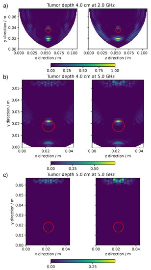
Figure 6.
The confocal maps showing particular artifacts and features. (a) ghost-like artifact for a 4 cm deep target at 2 GHz. (b) undersized target for a 4 cm deep target at 5 GHz. (c) no target for a 5 cm deep target at 5 GHz with a antenna grid.
These artifacts and features were common to all the antenna grids. Figure 7 shows in which range of frequencies and target depths the artifacts appeared. At the lowest frequencies, below circa 1 GHz, independently of the target depth, the main artifact was the appearance of rings in the confocal map as those of Figure 5. At higher frequencies this artifact appeared only when the target was in a shallow position up to 1–2 cm of depth. The appearance of a ghost target was visible at 1 GHz with deep targets and at higher frequencies at all depths. The maps that showed a too-small target or no target at all were those made at the highest frequencies and at the highest depths. This distribution of artifacts and features was in common to all the simulations with different antenna grids, however with minor variations.
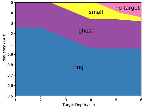
Figure 7.
General distribution of the artifacts relatively to central frequency and target depth.
There are several reasons behind the artifacts. The rings of Figure 5 were given by the strong interaction between the central antennas and the target. In fact the distance between the target and those antennas was comparable to the wavelength of the electromagnetic pulse. This can be observed in Figure 4d), where the signal coming from the central antenna was much more intense than that for the other antennas and therefore contributed more heavily to the formation of the confocal map. For shallow targets, there was a large difference in distances from the target between the central antenna and the lateral ones. However, this phenomenon became weaker and weaker with the depth (see the Supplementary Information SI) in agreement with the fact that only at short distances the target still resided in the antenna near-field. In fact, these artifacts appeared at the lowest frequencies or at the lowest depths.
The appearance of a ghost target (Figure 6a) at higher depths instead was associated with the low dielectric contrast between the target and the surrounding medium. In fact, the ghost represented the backscattering given by the bottom of the target. As it can be seen from Figure 4, the second echo was temporally separated from the first one, but still displayed similar amplitude. This was a consequence of the low attenuation of the electromagnetic wave inside the target compared with the surrounding medium. Since the dielectric permittivity of the medium increased with the frequency, the time separation between the first and the second echo, dependent on the phase velocity, became larger at larger frequencies (see SI). Furthermore, the intensity of the second echo was actually amplified by the integration performed in the reconstruction algorithm (DAS). Additionally, the ghost disappeared when the target was substitute with a perfectly conductive one for which there is no echo at the bottom of the target (see SI). Summarizing, this artifact was present only at intermediated frequencies for high target depths and because of the strong attenuation of the medium at high frequencies (see Figure 1b), it was not visible at high frequencies for deep targets.
The fact that the target appeared much smaller and at shallower positions than the original one (Figure 6b) was connected with the shortening of the wavelength at high frequencies. In fact, as it can be seen from Figure 4 the modulations in intensity belonging to a particular echo extended for a certain length of time which translated to a certain span in space in the confocal map. This span was connected with the wavelength of the signal used: at higher frequencies, i.e., smaller wavelength, the time extend of the modulation was shorter (see SI for an example), which is in agreement with the idea that shorter wavelengths correspond to higher spatial resolution. Considering the increase in the attenuation at high frequencies (Figure 1b) in these conditions it was only possible to localize the very top part of the target.
Increasing the depth of the target, the electromagnetic attenuation given by the lung tissue was too high to allow any signal to travel back from the target, which is in agreement with the fact that the disappearing of the target from the confocal map (Figure 6c) happened only at the highest frequencies and at the largest depths.
To quantify in which frequency range and nodule depth the cancer localization was possible, the confocal map was split into two regions and ; the first corresponds to the position of the expected target, the latter covers the remaining of the confocal map. To account for blurring effects, was taken as 10% larger than the real target. For both regions the averaged pixel intensity was calculated and the ratio R was chosen as a quantitative indicator of the goodness of the target localization:
where represents the pixel intensity averaged on all the region V. Ideally, the confocal map should not show any signal intensity apart from the expected location of the target giving an R value approaching infinity as . In the case of a very poor localization, instead, a considerable amount of signal appears also at positions not coinciding with the target position. In which case is close to zero and is a large number, bringing the ratio R close to zero.
The ratio R was calculated for all the confocal maps performed. There were three antennas grids distributions (, , and , i.e., with nine antennas, 16 antennas, and 25 antennas) and for every distribution the central frequency and the depth of the target was changed, between 500 MHz and 5 GHz and between 1 and 6 cm, respectively. This accounted for 180 confocal images. The ratio R for all these images is displayed as contour maps in Figure 8 separated by the three antenna distributions. The abscissa corresponds to the depth of the target, while the ordinate corresponds to the central frequency of the pulse reported in log scale. The dark part of the contour map represents a combination of pulse frequency and target depth which gave a low ratio R and therefore a poor localization of the target in those conditions. On the other side, the bright part of the contour map represents the conditions necessary for a good localization.
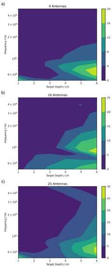
Figure 8.
Ratio R between the mean intensity at the expected target position and the rest of the map for (a), (b), and (c) antennas distributions.
There is a large variation in the accuracy in the localization of the pulmonary nodule by microwave imaging as given by the large variation in R which varied between some decimals and few decades as a maximum value. In particular, the , with a value of 20, shows the lowest maximum value, while the shows the highest. In general, an R value above 15 represented a good localization and a value of circa 10–15 a mediocre localization.
The larger values in the antenna grid were in agreement with the larger number of antennas in this configuration, which enhanced the localization and therefore suppressed the background.
All in all, the best localization appeared at the lowest frequencies and for the deepest targets. However, there are some differences between the antenna distributions. For the , (Figure 8c), the highest values of R were between 0.5 and 0.8 GHz and 5 to 6 cm of depth. Similar for , however with higher values of R. For the , instead, the highest R were at 0.9 GHz. This can be explained by the fact that in the the ring artifacts were slightly lower than with the and grids because there was no central antenna located exactly above the target, which were those producing the strongest rings artifacts as previously explained.
In all cases, the localization was very poor for shallow targets, below 3 cm, and high frequencies, above 2 GHz. Only exception the confocal map at 0.5 GHz, 1 cm target depth, and , which shows an R value circa 20. This particular map was affected by intense ring artifacts localized around the target location which produced an extremely high value of compared to .
Clearly, the most important factor in the reconstruction of meaningful confocal maps was the attenuation of the electromagnetic waves at the highest frequencies and the strong interaction between the target and the antennas at the lowest depths. Whereas the number of antennas played a secondary role in improving an already good localization, but did not change either the frequency nor the target depth at which the localization worked.
Furthermore, the effect of a smaller target was investigated (see SI) and we found that even a nodule of 2.5 mm in radius could be identified in the confocal images at a depth of 4 cm and at 0.6 GHz. The R value, in this case, was 23.3 against 26.3 for the 5 mm target radius. This shows that even if the wavelength at 0.6 GHz is 6.7 cm (see Figure 1) since the target was located in the near-field of the antennas it could still be localized.
To further investigate the performance of this localization method, some simulations were repeated for the best conditions, i.e., 0.6 GHz and antenna distribution, up to 10 cm of depth. Figure 9 reports these results which show how the ratio R increased up to more than 35 at 8 cm of the target depth and sharply decreased for further depths. This demonstrates how this localization could theoretically work for very deep nodules.
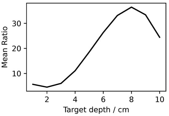
Figure 9.
Ratio R at 0.6 GHz for antenna distribution at different target depths.
4. Conclusions
In this article, the influence of several parameters, such as frequency, lesion depth, and number of acquisitions, was investigated for the localization of lung nodule by microwave imaging. This was studied through finite difference time domain (FDTD) simulations where a simple monostatic antenna was placed in contact with the lung tissue. A deflated lung was assumed as a medium to mimic the case during a thoracoscopic surgery and a pulmonary nodule was approximated by a sphere with different dielectric properties.
Several antenna grids were investigated spanning from to . In all the simulations, the nodule was positioned between 1 and 6 cm below the lung surface and the frequency of the microwave pulse was varied between 0.5 and 5 GHz.
The results show that the best localizations were those performed for deep pulmonary nodules, between 5 and 6 cm of depth, and at the lowest frequencies, below 1 GHz.
At lower depths, some artifacts appeared in the confocal images hindering the localization and at the highest frequencies, the attenuation given by the lung tissue was too strong to show any meaningful target in the confocal images.
However, despite the strong attenuation of the lung tissue and the low dielectric contrast between the tissue and the nodule, on theoretical ground, deep pulmonary nodules could be successfully localized through microwave imaging, even though a very simple antenna model without any directionality was used.
The best performances were found for 0.6 GHz for a antenna grid and showed that the nodule localization was possible up to 10 cm of depth.
This work gives some first guidelines for the usage of microwave imaging directly in the proximity of the lung which could be implemented in a thoracoscopic surgery as a simple and non-invasive method.
Further refinements are necessary to really establish the limit of this technique. In fact, higher working frequencies are preferred because of their improved spatial resolution and a more sophisticated antenna and a less homogeneous and ideal lung model should be used to realistically mimic the surgery condition. Moreover, different strategies can be employed to identify also those nodules that lay in shallow positions, as for example to change the distance between the antennas and the lung tissue, or to use spacing materials with predefined dielectric properties. Furthermore, measurements done at different frequencies could be used to improve accuracy. Finally, testing with tissue samples is foreseen in order to confirm and refine the numerical results.
Supplementary Materials
The following are available online at https://www.mdpi.com/article/10.3390/app11094282/s1.
Author Contributions
Investigation, A.B.; writing—original draft preparation, A.B.; writing—review and editing, P.P.P. and K.M.; funding acquisition, K.M. All authors have read and agreed to the published version of the manuscript.
Funding
This research was partially funded by BMBF grant number FKZ: 13FH5I05IA COHMED-DigiMed-OP and grant AIRLobe funded by “Innovative Projects” MWK-BW.
Institutional Review Board Statement
Not applicable.
Informed Consent Statement
Not applicable.
Conflicts of Interest
The authors declare no conflict of interest. The funders had no role in the design of the study; in the collection, analyses, or interpretation of data; in the writing of the manuscript, or in the decision to publish the results.
References
- Worldwide Cancer Data. 2018. Available online: https://www.wcrf.org/dietandcancer/cancer-trends/worldwide-cancer-data (accessed on 23 June 2020).
- Bray, F.; Ferlay, J.; Soerjomataram, I.; Siegel, R.L.; Torre, L.A.; Jemal, A. Global Cancer Statistics 2018: GLOBOCAN Estimates of Incidence and Mortality Worldwide for 36 Cancers in 185 Countries. CA Cancer J. Clin. 2018, 68, 394–424. [Google Scholar] [CrossRef]
- Siegel, R.L.; Miller, K.D.; Jemal, A. Cancer Statistics, 2016. CA Cancer J. Clin. 2016, 66, 7–30. [Google Scholar] [CrossRef]
- Keating, J.; Singhal, S. Novel Methods of Intraoperative Localization and Margin Assessment of Pulmonary Nodules. Semin. Thorac. Cardiovasc. Surg. 2016, 28, 127–136. [Google Scholar] [CrossRef] [PubMed]
- Ost, D.; Fein, A.M.; Feinsilver, S.H. The Solitary Pulmonary Nodule. N. Engl. J. Med. 2003, 348, 2535–2542. [Google Scholar] [CrossRef]
- Gould, M.K.; Donington, J.; Lynch, W.R.; Mazzone, P.J.; Midthun, D.E.; Naidich, D.P.; Wiener, R.S. Evaluation of Individuals with Pulmonary Nodules: When Is It Lung Cancer?: Diagnosis and Management of Lung Cancer, 3rd ed.: American College of Chest Physicians Evidence-Based Clinical Practice Guidelines. Chest 2013, 143, e93S–e120S. [Google Scholar] [CrossRef]
- Shennib, H. Intraoperative localization techniques for pulmonary nodules. Ann. Thorac. Surg. 1993, 56, 745–748. [Google Scholar] [CrossRef]
- Nakashima, S.; Watanabe, A.; Obama, T.; Yamada, G.; Takahashi, H.; Higami, T. Need for Preoperative Computed Tomography-Guided Localization in Video-Assisted Thoracoscopic Surgery Pulmonary Resections of Metastatic Pulmonary Nodules. Ann. Thorac. Surg. 2010, 89, 212–218. [Google Scholar] [CrossRef] [PubMed]
- Matsumoto, S.; Hirata, T.; Ogawa, E.; Fukuse, T.; Ueda, H.; Koyama, T.; Nakamura, T.; Wada, H. Ultrasonographic Evaluation of Small Nodules in the Peripheral Lung during Video-Assisted Thoracic Surgery (VATS). Eur. J. Cardio-Thorac. Surg. 2004, 26, 469–473. [Google Scholar] [CrossRef] [PubMed]
- Santambrogio, R.; Montorsi, M.; Bianchi, P.; Mantovani, A.; Ghelma, F.; Mezzetti, M. Intraoperative Ultrasound during Thoracoscopic Procedures for Solitary Pulmonary Nodules. Ann. Thorac. Surg. 1999, 68, 218–222. [Google Scholar] [CrossRef]
- Gabriel, C.; Gabriel, S.; Corthout, E. The Dielectric Properties of Biological Tissues: I. Literature Survey. Phys. Med. Biol. 1996, 41, 2231–2249. [Google Scholar] [CrossRef] [PubMed]
- Gabriel, C. Compilation of the Dielectric Properties of Body Tissues at RF and Microwave Frequencies; Technical Report; Department of Physics, King’s Coll London: London, UK, 1996. [Google Scholar]
- Gabriel, S.; Lau, R.W.; Gabriel, C. The Dielectric Properties of Biological Tissues: III. Parametric Models for the Dielectric Spectrum of Tissues. Phys. Med. Biol. 1996, 41, 2271–2293. [Google Scholar] [CrossRef]
- Gabriel, S.; Lau, R.W.; Gabriel, C. The Dielectric Properties of Biological Tissues: II. Measurements in the Frequency Range 10 Hz to 20 GHz. Phys. Med. Biol. 1996, 41, 2251–2269. [Google Scholar] [CrossRef]
- IT’IS Foundation. Tissue Properties Database V4.0; IT’IS Foundation: Zurich, Switzerland, 2018. [Google Scholar] [CrossRef]
- Fear, E.; Li, X.; Hagness, S.; Stuchly, M. Confocal Microwave Imaging for Breast Cancer Detection: Localization of Tumors in Three Dimensions. IEEE Trans. Biomed. Eng. 2002, 49, 812–822. [Google Scholar] [CrossRef] [PubMed]
- Hagness, S.; Taflove, A.; Bridges, J. Three-Dimensional FDTD Analysis of a Pulsed Microwave Confocal System for Breast Cancer Detection: Design of an Antenna-Array Element. IEEE Trans. Antennas Propag. 1999, 47, 783–791. [Google Scholar] [CrossRef]
- Meaney, P.; Fanning, M.; Li, D.; Poplack, S.; Paulsen, K. A Clinical Prototype for Active Microwave Imaging of the Breast. IEEE Trans. Microw. Theory Tech. 2000, 48, 1841–1853. [Google Scholar] [CrossRef]
- Babarinde, O.J.; Jamlos, M.; Ramli, N.B. UWB Microwave Imaging of the Lungs: A Review. In Proceedings of the 2014 IEEE 2nd International Symposium on Telecommunication Technologies (ISTT), Langkawi, Malaysia, 24–26 November 2014; pp. 188–193. [Google Scholar] [CrossRef]
- Babarinde, O.; Jamlos, M.; Soh, P.; Schreurs, D.P.; Beyer, A. Microwave Imaging Technique for Lung Tumour Detection. In Proceedings of the 2016 German Microwave Conference (GeMiC), Bochum, Germany, 14–16 March 2016; pp. 100–103. [Google Scholar] [CrossRef]
- Wang, J.R.; Sun, B.Y.; Wang, H.X.; Pang, S.; Xu, X.; Liu, Q. Experimental Study of Dielectric Properties of Human Lung Tissue in Vitro. J. Med. Biol. Eng. 2014, 34, 598–604. [Google Scholar] [CrossRef]
- Battistel, A.; Möller, K. Ultra-Wideband Localization of Pulmonary Nodules During Thoracoscopic Surgery. In Proceedings of the EMBEC2020, Portorož, Slovenia, 29 November 29–3 December 2020. [Google Scholar]
- Giannopoulos, A. Modelling Ground Penetrating Radar by GprMax. Constr. Build. Mater. 2005, 19, 755–762. [Google Scholar] [CrossRef]
- Warren, C.; Giannopoulos, A.; Giannakis, I. gprMax: Open Source Software to Simulate Electromagnetic Wave Propagation for Ground Penetrating Radar. Comput. Phys. Commun. 2016, 209, 163–170. [Google Scholar] [CrossRef]
- Yee, K. Numerical Solution of Initial Boundary Value Problems Involving Maxwell’s Equations in Isotropic Media. IEEE Trans. Antennas Propag. 1966, 14, 302–307. [Google Scholar] [CrossRef]
- Cheng, D.K. Fundamentals of Engineering Electromagnetics, 1st ed.; Prentice Hall: Hoboken, NJ, USA, 1992. [Google Scholar]
- Li, X.; Hagness, S. A Confocal Microwave Imaging Algorithm for Breast Cancer Detection. IEEE Microw. Wirel. Compon. Lett. 2001, 11, 130–132. [Google Scholar] [CrossRef]
- Elahi, M.; O’Loughlin, D.; Lavoie, B.; Glavin, M.; Jones, E.; Fear, E.; O’Halloran, M. Evaluation of Image Reconstruction Algorithms for Confocal Microwave Imaging: Application to Patient Data. Sensors 2018, 18, 1678. [Google Scholar] [CrossRef] [PubMed]
- Kouzaki, T.; Kimoto, K.; Kubota, S.; Toya, A.; Sasaki, N.; Kikkawa, T. Quasi Yagi-Uda Antenna Array for Detecting Targets in a Dielectric Substrate. In Proceedings of the 2009 IEEE International Conference on Ultra-Wideband, Vancouver, BC, Canada, 9–11 September 2009; pp. 759–762. [Google Scholar] [CrossRef]
- Mario, V.; Morabito, F.; Angiulli, G. Adaptive Image Contrast Enhancement by Computing Distances into a 4-Dimensional Fuzzy Unit Hypercube. IEEE Access 2017, 5, 26922–26931. [Google Scholar] [CrossRef]
- Orujov, F.; Maskeliunas, R.; Damasevicius, R.; Wei, W. Fuzzy based image edge detection algorithm for blood vessel detection in retinal images. Appl. Soft Comput. 2020, 94, 106452. [Google Scholar] [CrossRef]
Publisher’s Note: MDPI stays neutral with regard to jurisdictional claims in published maps and institutional affiliations. |
© 2021 by the authors. Licensee MDPI, Basel, Switzerland. This article is an open access article distributed under the terms and conditions of the Creative Commons Attribution (CC BY) license (https://creativecommons.org/licenses/by/4.0/).