Global Stability Analysis of the Model of Series/Parallel Connected CSTRs with Flow Exchange Subject to Persistent Perturbation on the Input Concentration

Abstract

In this paper, we study the convergence properties of a network model comprising three continuously stirred tank reactors (CSTRs) with the following features: (i) the first and second CSTRs are connected in series, whereas the second and third CSTRs are connected in parallel with flow exchange; (ii) the pollutant concentration in the inflow to the first CSTR is time varying but bounded; (iii) the states converge to a compact set instead of an equilibrium point, due to the time varying inflow concentration. The practical applicability of the arrangement of CSTRs is to provide a simpler model of pollution removal from wastewater treatment via constructed wetlands, generating a satisfactory description of experimental pollution values with a satisfactory transport dead time. We determine the bounds of the convergence regions, considering these features, and also: (i) we prove the asymptotic convergence of the states; (ii) we determine the effect of the presence of the side tank (third tank) on the transient value of all the system states, and we prove that it has no effect on the convergence regions; (iii) we determine the invariance of the convergence regions. The stability analysis is based on dead zone Lyapunov functions, and comprises: (i) definition of the dead zone quadratic form for each state, and determination of its properties; (ii) determination of the time derivatives of the quadratic forms and its properties. Finally, we illustrate the results obtained by simulation, showing the asymptotic convergence to the compact set.

1. Introduction

Several systems converge to a compact set instead of an equilibrium point, for instance: (i) chaotic systems [1,2,3]; (ii) closed-loop systems subject to external disturbances or model uncertainties [4,5,6,7], or input saturation [8,9,10]. For this type of system, the global stability analysis considers large but bounded initial values of the state variables, and comprises determining the convergence region of the state variables, proving asymptotic or exponential global stability, and proving the invariance of the convergence region [2,3]. To this end, the Lyapunov function can be used, which consists of a radially unbounded function, possibly a quadratic form.

There are three common approaches based on the Lyapunov function for studying the aforementioned systems converging to compact sets. In the first approach, the Lyapunov function is positive definite, and can include quadratic forms of states with some deviation. The expression of the time derivative of the Lyapunov function is arranged as a first order differential equation, and it is concluded that the Lyapunov function converges exponentially to a compact set [2,3,11]. As an example, in Zhang (2017), the stability of a Lorenz system is determined for three different ranges of a model parameter [3]. This system consists of three ordinary differential equations (ODEs). In Liao (2017), the stability of a Yang-Chen system is analyzed [2]. The system consists of three ODE’s with states x, y, z. Global stability of both compact sets and equilibrium points are studied. To study global exponential convergence to compact sets, different radially unbounded Lyapunov functions are constructed for different quadrant regions of the state plane. Also, the ranges of a model parameter that imply global stability or instability of the equilibrium points are determined.

In the second approach, the Lyapunov function is positive definite and the expression of the time derivative of the Lyapunov function is negative when the state variables are outside the convergence region. It is concluded that the system converges asymptotically [3,11].

The third approach comprises dead-zone radially unbounded positive functions. This approach has been traditionally used for robust control design, but not for open-loop systems. An early development is presented in [12,13,14], and further developments in [15,16,17]. The main advantages of this approach are: (i) it allows rigorous proof of the asymptotic convergence to compact sets, through Barbalat’s lemma; (ii) it facilitates stability analysis for the case that asymptotic but not exponential convergence occurs [16,17,18]. In Rincon (2020), this approach was used to determine the convergence of a continuously stirred tank reactor (CSTR) open-loop system that comprises three reactions in the presence of an external disturbance [19]. This system is described by three cascaded differential equations whose states converge to a compact set. In the particular case of bioreaction systems, there are several global stability studies, proving convergence to equilibrium points, but not the convergence to compact set [20,21,22].

Another result of global stability analysis for systems converging to compact sets is BIBO stability. It can be performed for the case of bounded or L₂ disturbances, and it results in an input–output relationship that relates the system output or states in terms of either the input signal or the time integral of the squared input signal, where the input signal may be an external disturbance or a manipulated input. This expression is obtained by integrating the time derivative of the Lyapunov function. A BIBO stability study for an open loop system is presented in [23], where a non-linear Caputo fractional system with time varying bounded delay is considered. A quadratic Lyapunov function is defined, and the resulting fractional derivative is a function of the negative Lyapunov function. As a consequence of this expression, the upper bound of the Lyapunov function, system states and system output are a function of the upper bound of the input.

BIBO stability is also determined for closed loop systems (see [24,25,26,27,28]). In [24], a semi-active controller is formulated for a vibrating structure. The Lyapunov analysis is combined with passivity theory and uses a storage function as a Lyapunov function. The BIBO stability result relates the displacements and velocities as a function of L₂ external forces. Also, the ranges of the controller parameters that lead to BIBO stability are defined. In [25], a robust observer-based controller design is formulated for a class of nonlinear systems described by Tagaki–Sugeno (TS) models, subject to persistent bounded external disturbance. A non-quadratic Lyapunov function is used. The BIBO stability result relates the closed loop states as a function of the external disturbance. In [26], an adaptive neural controller is developed for a n-link rigid robotic manipulator. Neural networks are used for approximating the unknown dynamics, and the backstepping strategy is used as a basic control framework. As a result of the controller design, the overall Lyapunov function (V₂) comprises the subsystem Lyapunov functions associated to the z_i states and the parameter updating error. The dV₂/dt expression is a function of V₂, so that it is concluded that the zi states converge to compact sets whose width depends on the neural approximation error.

In this paper, we study the stability of a network model comprising three CSTRs with the following features: (i) the pollutant concentration in the inflow to the first CSTR is time varying; (ii) the first and second CSTRs are connected in series, whereas the second and third CSTRs are connected in parallel with flow exchange; (iii) the states converge to a compact set instead of an equilibrium point. The practical applicability of the arrangement of CSTRs is to provide a simpler model of pollution removal from wastewater treatment via constructed wetlands, generating a satisfactory description of experimental pollution values with a satisfactory transport dead time. The aforementioned features make the global stability analysis complex. The convergence sets of the system states are determined as a function of the concentration of the inflow to the first tank, and the global asymptotic convergence of the states to these sets and their invariant nature are proved. Also, the effect of the presence of flow exchange on the transient value of the system states is determined, and it is concluded that it has no effect on the convergence regions. The study is based on global stability using dead zone Lyapunov functions and Barbalat’s lemma.

The contribution of this work with respect to closely related studies on global stability of continuous stirred tank reactors (CSTR) are:

• we consider three connected CSTRs, including a side CSTR with flow exchange, whereas related studies consider a single CSTR with several states (e.g., biomass and substrate concentrations) [20,21,29,30];
• we consider the case that the system converges to a compact set, whereas related studies consider convergence to an equilibrium point [20,21,29,30].

The paper is organized as follows. The preliminaries and description of the model are presented in Section 2; the stability analysis is presented in Section 3, including the first tank (Section 3.1) and both the second and third tanks (Section 3.2). The numerical simulation is presented in Section 4, and the conclusions in Section 5.

2. Model Description

Modelling of constructed wetlands is complex because of the large number of processes involved in pollution removal, the hydraulics in a porous medium with the diffusive flow, and the dead time. In addition, the pollution removal is influenced considerably by the hydraulics and environmental conditions. The last generation of models (process—based models) are rigorous but overly complex, with difficult estimation of its parameters [31,32,33]. In contrast, series/parallel connection of CSTRs is simple and capable of describing transport dead time, diffusion and reaction [31].

In Marsili (2005), a simple model is proposed for describing the disperse hydraulics and pollution removal dynamics in horizontal subsurface constructed wetlands [31]. The structure of the hydraulic model comprises three series CSTRs, followed by two parallel CSTRs, and a plug flow reactor. The parallel CSTRs involve no flow exchange. The kinetics is of the Monod type, and only depends on the concentration of the modelled pollutant. The outlet and inlet flows of the system are the same, and the liquid CSTR volumes are constant. The model was fitted to both experimental tracer data and current (no tracer) data.

In Davies (2007) and Freire (2009), a simple modelling strategy is proposed for describing hydraulics and pollution removal dynamics corresponding to tracer data from vertical subsurface constructed wetlands [34,35]. The model comprises three CSTRs, the first and second CSTRs are connected in series, whereas the second and third CSTRs are connected in parallel with flow exchange. The inlet flow is considered different from the outlet flow, and no model is considered for it. The liquid volumes of the parallel CSTRs are constant, whereas the liquid volume of the first CSTR is considered varying and is described by a first-order differential equation that is fitted to experimental data. The specific reaction rate is of the first order and it only depends on the concentration of the modelled pollutant.

We use the global stability definition as follows.

Definition 1.

Consider the system dX/dt = f(X), where X = (x₁, x₂, …, x_n) ∈ $ℛ$ⁿ, f: $ℛ$ⁿ → $ℛ$ⁿ, X(t,t_o,X_o) denoted as X(t) is a solution to the system, and X₀ ∈ $ℛ$ⁿ is an initial value of X(t). Consider the compact set Ω_Q ⊂ $ℛ$ⁿ. Define the distance between the solution X and the compact set Ω_Q as:

$$\rho \left(X,{\Omega }_Q\right)=\underset{Y\in {\Omega }_Q}{inf}||X-Y||.$$

If for all X₀ satisfying X₀ ∈ $ℛ$ⁿ, X₀ ∉ Ω_Q the property $\underset{t\to \infty }{\lim }\rho \left(X,{\Omega }_Q\right)=0$ holds, then the compact set Ω_Q is called a global convergence set of the system, and the system is called globally asymptotically stable.

We consider a series/parallel CSTRs-based model for representing the hydraulics and pollution removal dynamics in subsurface constructed wetlands, resulting from a combination of the models proposed by [31,34]. A single pollutant and a time-varying inflow pollutant concentration are considered. The CSTRs connection comprises three CSTRs, the first and second CSTRs are connected in series, whereas the second and third CSTRs are connected in parallel with flow exchange (Figure 1). The mass balances for the CSTRs are:

$$\frac{d{S}_1}{dt}=\left(S_{in}-S_1\right)\frac{Q}{v_1}-r_{s1},$$

(1)

$$\frac{d{S}_2}{dt}=\left(S_1-S_2\right)\frac{Q}{v_2}-r_{s2}+\frac{Q_D}{v_2}\left(S_3-S_2\right),$$

(2)

$$\frac{d{S}_3}{dt}=\left(S_2-S_3\right)\frac{Q_D}{v_3},$$

(3)

$$S_{in}={\overline{S}}_{in}+{\delta }_{sin},$$

(4)

where $S_1$ is the pollutant concentration in CSTR 1; $S_2$ is the pollutant concentration in CSTR 2; $S_3$ is the pollutant concentration in CSTR 3; $S_{in}$ is the inlet pollutant concentration; $Q$ is the wastewater flow entering CSTR 1 and CSTR 2; $Q_D$ is the wastewater flow entering and leaving CSTR 3; $v_i$ is the liquid volume of the ith CSTR; $r_{s1}$ is the reaction rate of CSTR 1; $r_{s2}$ is the reaction rate of CSTR 2. In addition, $S_1$ is defined in ${ℝ}^{+},$ $S_2$ is defined in ${ℝ}^{+},$ $S_3$ is defined in ${ℝ}^{+}$.

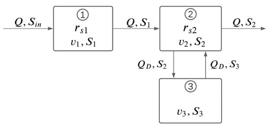
Figure 1. Schematic structure of the series/parallel continuously stirred tank reactor (CSTR)-based model.

Assumptions: 

Assumption 1.

$Q$,$Q_D$,$v_1$,$v_2$, and$v_3$are positive and constant. This implies that$Q/v_1$,$Q/v_2$,$Q_D/v_2$and$Q_D/v_3$are constant and positive.

Assumption 2.

${\overline{S}}_{in}$is positive and constant,${\delta }_{sin}$is varying but bounded,$max\left\{{\delta }_{sin}\right\}>0, min\left\{{\delta }_{sin}\right\}<0$.

Assumption 3.

The reaction rate r_s1 only depends on$S_1$, it is bounded for$S_1$bounded,$\frac{d{r}_{s1}}{d{S}_1}\ge 0$;$r_{s2}$only depends on$S_2$, it is bounded for$S_2$bounded, and$\frac{d{r}_{s2}}{d{S}_2}\ge 0$.

In the case of constant $S_{in}$, ${\delta }_{sin}$ = 0 in Equation (4), $S_1$ converges to $S_1^{eq}$, $S_2$ converges to $S_2^{eq}$ and $S_3$ converges to $S_3^{eq}$, where $S_1^{eq}$, $S_2^{eq}$ and $S_3^{eq}$ are positive constants obtained by equating Equations (1)–(3) to zero:

$$0=\left({\overline{S}}_{in}-S_1\right)\frac{Q}{v_1}-r_{s1},$$

(5)

$$0=\left(S_1-S_2\right)\frac{Q}{v_2}-r_{s2}+\frac{Q_D}{v_2}\left(S_3-S_2\right),$$

(6)

$$0=\left(S_2-S_3\right)\frac{Q_D}{v_3}.$$

(7)

Let

$$x_1=S_1-S_1^{eq},$$

(8)

$$x_2=S_2-S_2^{eq},$$

(9)

$$x_3=S_3-S_3^{eq}.$$

(10)

The $x_1$ dynamics is obtained by subtracting Equation (5) from Equation (1):

$$\frac{d{x}_1}{dt}=-D\left(x_1+\frac{r_{x1}}{D}-{\delta }_{sin}\right),$$

(11)

$$r_{x1}=r_{s1}-r_{s1}^{eq},$$

(12)

where $D=Q/v_1>0$, $r_{s1}^{eq}$ is $r_{s1}$ evaluated at $S_1=S_1^{eq}$.

The $x_2$ dynamics is obtained by subtracting Equation (6) from Equation (2):

$$\frac{d{x}_2}{dt}=\left(x_1-x_2\right)\frac{Q}{v_2}-r_{x2}-\frac{Q_D}{v_2}\left(x_2-x_3\right),$$

(13)

$$r_{x2}=r_{s2}-r_{s2}^{eq}.$$

(14)

The term $r_{s2}^{eq}$ is $r_{s2}$ evaluated at $S_2=S_2^{eq}$.

The $x_3$ dynamics is obtained by subtracting Equation (7) from Equation (3):

$$\frac{d{x}_3}{dt}=\left(x_2-x_3\right)\frac{Q_D}{v_3}.$$

(15)

In addition, $x_1$ is defined in [−$S_1^{eq}, \infty ), x_2$ is defined in [−$S_2^{eq}, \infty ),$ and $x_3$ is defined in [−$S_3^{eq}, \infty )$. The model is fitted to current (no tracer) data in Section 3.

3. Global Stability Analysis

In this section, the stability analysis is performed for the network model (1), including the determination of the convergence set, the asymptotic convergence and the invariance. The stability analysis is based on Lyapunov theory and Barbalat’s lemma. Recall that early global stability studies based on dead zone Lyapunov functions are presented in [12,13,14], whereas later studies are presented in [16,17,19].

A dead zone quadratic form $V_1$ is defined for the first state $x_1$, $V_2$ for the second state $x_2$ and $V_3$ for the third state $x_3$, and their properties are determined. An overall Lyapunov function V is defined as a weighted sum of the quadratic forms $V_1$, $V_2$, and $V_3$. The time derivative of each dead zone quadratic form is determined. The stability analysis of the first tank is independent of the other tanks, whereas the stability analysis of the second and third tanks is simultaneous and requires the stability results of the first tank.

3.1. Stability Analysis for the First Tank

The stability analysis is based on determining the non-positive nature of $d{V}_1/dt$, where $V_1$ is the dead-zone quadratic form for $x_1$. The function $V_1$ and its gradient $d{V}_1/d{x}_1$ are defined so as to achieve this goal.

The procedure comprises the following tasks: (i) determination of the expression for $d{V}_1/dt$; (ii) definition of the gradient $d{V}_1/d{x}_1$ and the dead zone quadratic form $V_1$ for the state $x_1$; (iii) arrangement of the $d{V}_1/dt$ expression in terms of a non-positive function of $d{V}_1/d{x}_1$; (iv) integration of the $d{V}_1/dt$ expression. The definition of the gradient $d{V}_1/d{x}_1$. and $V_1$ requires the determination of the $d{V}_1/dt$ expression and the properties of the terms involved.

Theorem 1.

Consider the model in Equations (11) and (12), subject to assumptions 1 to 3. (Ti) The state $x_1$ converges asymptotically to ${\mathit{\Omega }}_{x1}$, ${\mathit{\Omega }}_{x1}=\left\{x_1:x_1^l\le x_1\le x_1^u\right\}$, where $x_1^u=\left\{x_1:g_{x1}-max\left\{{\delta }_{sin}\right\}=0 \right\}$, $x_1^u>0$, $x_1^l=\left\{x_1:g_{x1}-min\left\{{\delta }_{sin}\right\}=0 \right\}, x_1^l<0$, and $g_{x1}=x_1+\frac{r_{x1}}{D}$, and $S_1$ converges asymptotically to ${\mathit{\Omega }}_{S1}$ where ${\mathit{\Omega }}_{S1}=\left[S_1^l S_1^u\right]$, $S_1^l=x_1^l+S_1^{eq}$, $S_1^u=x_1^u+S_1^{eq}$ and $S_1^{eq}$ is provided by Equation (5). (Tii) The sets ${\mathit{\Omega }}_{x1}$ and ${\mathit{\Omega }}_{S1}$ are invariant.

Proof. 

Task 1. Determination of the $d{V}_1/dt$ expression.

The time derivative of $V_1$ can be expressed as:

$$\frac{d{V}_1}{dt}=f_{v1}\frac{d{x}_1}{dt},$$

(16)

$$f_{v1}=\frac{d{v}_1}{d{x}_1}.$$

(17)

Incorporating the $x_1$ dynamics (11) and arranging, yields:

$$\frac{d{V}_1}{dt}=\left(-1\right)D{f}_{v1}\left(g_{x1}-{\delta }_{sin}\right),$$

(18)

where,

$$g_{x1}=x_1+\frac{r_{x1}}{D},$$

(19)

$$\frac{d{g}_{x1}}{d{x}_1}=1+\frac{1}{D}\frac{d{r}_{x1}}{d{x}_1}\ge 1.$$

(20)

□

Task 2.

Definition of the gradient $d{V}_1/d{x}_1$ and the dead zone quadratic form $V_1$ for the state $x_1$.

At what follows, we examine the properties of the term $g_{x1}-{\delta }_{sin}$ appearing in Equation (18). From Equations (12), (19) and (20) and Assumption 3 we have:

$$\frac{d{g}_{x1}}{d{x}_1}\ge 1; g_{x1}=0 for x_1=0; sgn\left(g_{x1}\right)=sgn\left(x_1\right),$$

(21)

$$g_{x1}-{\delta }_{sin}>0 for x_1>x_1^u,$$

(22)

$$g_{x1}-{\delta }_{sin}<0 for x_1<x_1^l,$$

(23)

where,

$$x_1^u=\left\{x_1:g_{x1}-max\left\{{\delta }_{sin}\right\}=0 \right\},x_1^u>0,$$

(24)

$$x_1^l=\left\{x_1:g_{x1}-min\left\{{\delta }_{sin}\right\}=0 \right\}, x_1^l<0.$$

(25)

Therefore,

$$sgn\left(g_{x1}-{\delta }_{sin}\right)=sgn\left(x_1\right)=sgn\left(g_{x1}\right) for x_1\notin \left[x_1^l,x_1^u\right].$$

(26)

To obtain non-positive $d{V}_1/dt$ in Equation (18), we need to choose $f_{v1}$ such that:

$$-f_{v1}\left(g_{x1}-{\delta }_{sin}\right)<0 for x_1 \notin \left[x_1^l,x_1^u\right],$$

(27)

$$-f_{v1}\left(g_{x1}-{\delta }_{sin}\right)=0 for x_1 \notin \left[x_1^l,x_1^u\right].$$

(28)

In view of properties (26) and to fulfill conditions (27) and (28), we choose:

$$f_{v1}=\{\begin{array}{c}{x}_1-x_1^u for x_1>x_1^u\\ 0 for x_1 \in \left[x_1^l,x_1^u\right].\\ x_1-x_1^l for x_1<x_1^l\end{array}$$

(29)

The main properties of $f_{v1}$ are:

$$\left(Pi\right)f_{v1} is continuous with respect to x_1 ,$$

(30)

$$(Pii) f_{v1}=0 for x_1 \in \left[x_1^l,x_1^u\right],$$

(31)

$$\left(Piii\right) f_{v1}\ne 0 for{ x}_1 \notin \left[x_1^l,x_1^u\right],$$

(32)

$$P\left(iv\right) sgn\left(f_{v1}\right)=sgn\left(x_1\right)\ne 0 for{ x}_1 \notin \left[x_1^l,x_1^u\right],$$

(33)

$$\left(Pv\right) sgn\left(f_{v1}\right)=sgn\left(g_{x1}\right)=sgn\left(g_{x1}-{\delta }_{sin}\right)\ne 0 for{ x}_1 \notin \left[x_1^l,x_1^u\right].$$

(34)

A dead-zone Lyapunov function that satisfies $d{V}_1/d{x}_1=f_{v1}$ (Equation (17)) is:

$$V_1=\frac{1}{2}{f}_{v1}^2.$$

(35)

The main properties of $V_1$ are:

$$V_1>0 for x_1 \notin \left[x_1^l,x_1^u\right],$$

(36)

$$V_1=0{ for x}_1\in \left[x_1^l,x_1^u\right].$$

(37)

□

Task 3.

Arrangement of the $d{V}_1/dt$ expression in terms of a non-positive function of $f_{v1}=d{V}_1/d{x}_1$.

From properties (31), (34), it follows that the term $f_{v1}\left(g_{x1}-{\delta }_{sin}\right)$ appearing in Equation (18) satisfies:

$$f_{v1}\left(g_{x1}-{\delta }_{sin}\right)=|f_{v1}||\left(g_{x1}-{\delta }_{sin}\right)|\ge 0.$$

(38)

From the definition of $g_{x1}$ (19) and definitions of $x_1^l, x_1^u$ (24), (25), it follows that:

$$\lfloor g_{x1}-{\delta }_{sin}\rfloor \ge |g_{t1}|,$$

(39)

$$g_{t1}=\{\begin{array}{c}{g}_{x1}-max\left\{{\delta }_{sin}\right\} for x_1>x_1^u\\ 0 for x_1\in \left[x_1^l, x_1^u\right]\\ g_{x1}-min\left\{{\delta }_{sin}\right\} for x_1<x_1^l\end{array}.$$

(40)

From Equations (38) and (39), it follows that:

$$f_{v1}\left(g_{x1}-{\delta }_{sin}\right)\ge |f_{v1}||g_{t1}|=f_{v1}{g}_{t1}\ge 0.$$

(41)

From the property (21), definition of $g_{t1}$ (40), and definition of $f_{v1}$ (29), it follows that:

$$|g_{t1}|\ge |f_{v1}|.$$

(42)

Therefore, Equation (41) yields:

$$f_{v1}\left(g_{x1}-{\delta }_{sin}\right)\ge f_{v1}^2\ge 0.$$

(43)

Using this in Equation (18) yields:

$$\frac{d{V}_1}{dt}\le -D{f}_{v1}^2.$$

(44)

Accounting for the definition of $V_1$ (35), we have:

$$\frac{d{V}_1}{dt}\le -2D{V}_1\le 0.$$

□

Task 4.

Integration of the $d{V}_1/dt$ expression.

From the above expression, it follows that:

$$V_1\le V_{1to}{e}^{-2D\left(t-t_o\right)}.$$

(45)

That is, $V_1$(35) converges exponentially to zero, and consequently $f_{v1}$ converges exponentially to zero. Further, accounting for the definition of $f_{v1}$ (29), it follows that $x_1$ converges asymptotically to ${\Omega }_{x1}=\left\{x_1:x_1^l\le x_1\le x_1^u\right\}$. From this convergence result and the definition of $x_1$ (8), it follows that $S_1$ converges asymptotically to ${\Omega }_{S1}$; where,

$${\Omega }_{S1}=\left[S_1^l\hspace{1em}{S}_1^u\right],$$

(46)

$$S_1^l=x_1^l+S_1^{eq}, S_1^u=x_1^u+S_1^{eq} .$$

(47)

$S_1^{eq}$ is provided by Equation (5), the bounds $x_1^l$, $x_1^u$ are defined in Equations (24) and (25). This completes the proof of Ti.

From Equation (44) and properties (31) and (32), it follows that $\frac{d{V}_1}{dt}<0 for x_1 \notin {\Omega }_{x1}$ and $\frac{d{V}_1}{dt}\le 0 for x_1\in {\Omega }_{x1}$. Therefore, the set ${\Omega }_{x1}$ is invariant, and consequently, ${\Omega }_{s1}$ is invariant. This completes the proof of Tii. □

Remark 1.

The property $|g_t|\ge |f_{v1}|$ (42) is crucial for proving the asymptotic convergence of x₁.

Remark 2.

The invariance of the set ${\mathit{\Omega }}_{s1}$ stated in Theorem 1 implies that once the state $S_1$ is inside the convergence region ${\mathit{\Omega }}_{s1}$, that is, $S_1\in {\mathit{\Omega }}_{s1}$, it remains inside afterwards.

3.2. Stability Analysis for the Second and Third Tanks

The stability analysis and majorly the proof for asymptotic convergence of $x_2$ and $x_3$ to their compact sets, is based on determining the non-positive nature of $dV/dt=d{V}_1/dt+k_{2}d{V}_2/dt+k_{3}d{V}_3/dt$, where $V=V_1+k{V}_2+k{V}_3$, $V$ is the overall Lyapunov function, $V_2$ is the dead zone quadratic form for the state $x_2$ and $V_3$ the dead zone quadratic form for the state $x_3$, and $k_2$ and $k_3$ are positive constants. To achieve this goal, the functions $V_2$ and $V_3$ and the gradients $d{V}_2/d{x}_2$ and $d{V}_3/d{x}_3$ are defined accordingly, and the non-positive nature of the terms of the $dV/dt$ expression is determined.

The procedure comprises the following tasks: (i) determination of the expression for $d{V}_2/dt+kd{V}_3/dt$; (ii) arrangement of the expression for $d{V}_2/dt+kd{V}_3/dt$ in terms of $f_{v1}$; (iii) definition of gradient $d{V}_2/d{x}_2$ and dead zone quadratic form $V_2$; (iv) arrangement of the expression for $d{V}_2/dt+kd{V}_3/dt$ in terms of a non-positive function of $d{V}_2/d{x}_2$; (v) definition of gradient $d{V}_3/d{x}_3$ and dead zone quadratic form $V_3$; (vi) definition of the overall Lyapunov function V and determination of the non-positive nature of the expression for $dV/dt=d{V}_1/dt+kd{V}_2/dt+kd{V}_3/dt$; (vii) integration of the $dV/dt$ expression. The definition of the gradients $d{V}_2/d{x}_2$ and $d{V}_3/d{x}_3$ and the quadratic forms $V_2$ and $V_3$ requires the determination of the expression for $d{V}_2/dt+kd{V}_3/dt$ and the properties of the terms involved.

Theorem 2.

Consider the model (11)–(15), subject to assumptions 1 to 3. (Ti) the state $x_2$ converges asymptotically to ${\mathit{\Omega }}_{x2}$, ${\mathit{\Omega }}_{x2}=\left\{x_2:x_2^l\le x_2\le x_2^u\right\}$, where:

$$\begin{gathered} x_2^u=\left\{x_2: g_{x2}-max\left\{{\delta }_2\right\}=0\right\}, x_2^u>0 \\ {x}_2^l=\left\{x_2: g_{x2}-min\left\{{\delta }_2\right\}=0\right\}, x_2^l<0 \\ {g}_{x2}=x_2+\frac{r_{x2}}{Q/v_2},{\delta }_2=-d_{x1}, \\ {d}_{x1}=\{\begin{array}{c}-x_1^u for x_1>x_1^u\\ -x_1 for x_1 \in \left[x_1^l, x_1^u\right]\\ -x_1^l for x_1<x_1^l\end{array}. \end{gathered}$$

$S_2$converges asymptotically to ${\mathit{\Omega }}_{S2}$ where ${\mathit{\Omega }}_{S2}=\left[S_2^l S_2^u\right]$, $S_2^l=x_2^l+S_2^{eq}$, $S_2^u=x_2^u+S_2^{eq}$ and $S_2^{eq}$ is provided by Equations (5)–(7). (Tii) the state x₃ converges asymptotically to ${\mathit{\Omega }}_{x3}$, ${\mathit{\Omega }}_{x3}=\left\{x_3:x_3^l\le x_3\le x_3^u\right\}$, where $x_3^u=x_2^u; x_3^l=x_2^l$, and $S_3$ converges asymptotically to ${\mathit{\Omega }}_{S3}$ where ${\mathit{\Omega }}_{S3}=\left[S_3^l S_3^u\right]$, $S_3^l=x_3^l+S_3^{eq}$, $S_3^u=x_3^u+S_3^{eq}$ and $S_3^{eq}$ is provided by Equations (5)–(7). (Tiii) The sets ${\mathit{\Omega }}_x={\mathit{\Omega }}_{x1}{{\displaystyle \bigcup }}^{ }{\mathit{\Omega }}_{x2}{{\displaystyle \bigcup }}^{ }{\mathit{\Omega }}_{x3}$ and ${\mathit{\Omega }}_S={\mathit{\Omega }}_{S1}{{\displaystyle \bigcup }}^{ }{\mathit{\Omega }}_{S2}{{\displaystyle \bigcup }}^{ }{\mathit{\Omega }}_{S3}$ are invariant.

Proof. 

Task 1. Determination of the expression for $d{V}_2/dt+kd{V}_3/dt$.

The $d{x}_2/dt$ expression (13) can be rewritten as:

$$\frac{d{x}_2}{dt}=-\frac{Q_D}{v_2}\left(x_2-x_3\right)+\left(-1\right)\frac{Q}{v_2}\left(g_{x2}-x_1\right),$$

(48)

where:

$$g_{x2}=x_2+\frac{r_{x2}}{Q/v_2}.$$

(49)

The time derivative of $V_2$ can be expressed as:

$$\frac{d{V}_2}{dt}=f_{v2}\frac{d{x}_2}{dt},$$

(50)

$$f_{v2}=\frac{d{V}_2}{d{x}_2}.$$

(51)

Substituting the $d{x}_2/dt$ expression (Equation (48)) and arranging, yields:

$$\frac{d{V}_2}{dt}=f_{v2}\left(-1\right)\frac{Q_D}{v_2}\left(x_2-x_3\right)+\left(-1\right)\frac{Q}{v_2}{f}_{v2}\left(g_{x2}-x_1\right).$$

(52)

The time derivative of $V_3$ can be expressed as:

$$\frac{d{V}_3}{dt}=f_{v3}\frac{d{x}_3}{dt},$$

(53)

$$f_{v3}=\frac{d{V}_3}{d{x}_3}.$$

(54)

Substituting the $d{x}_3/dt$ expression (Equation (15)) and arranging, yields

$$\frac{d{V}_3}{dt}=f_{v3}\left(\left(x_2-x_3\right)\frac{Q_D}{v_3}\right).$$

(55)

Hence,

$$\frac{d}{dt}\left(\frac{v_3}{v_2}{V}_3\right)=f_{v3}\left(\left(x_2-x_3\right)\frac{Q_D}{v_2}\right).$$

(56)

Adding $d{V}_2/dt$ (52) and $d{V}_3/dt$ (56), yields

$$\frac{d{V}_2}{dt}+\frac{d}{dt}\left(\frac{v_3}{v_2}{V}_3\right)=\left(-1\right)\frac{Q_D}{v_2}\left(x_2-x_3\right)\left(f_{v2}-f_{v3}\right)+\left(-1\right)\frac{Q}{v_2}{f}_{v2}\left(g_{x2}-x_1\right).$$

(57)

□

Task 2.

Arrangement of the expression for $d{V}_2/dt+kd{V}_3/dt$ in terms of $f_{v1}$.

The $x_1$ signal appearing in Equation (57) can be expressed as the sum of $f_{v1}$ and a disturbance term. Let,

$$d_{x1}=f_{v1}-x_1.$$

(58)

Using the definition of $f_{v1}$ (29), we have:

$$d_{x1}=\{\begin{array}{c}-x_1^u for x_1>x_1^u\\ -x_1 for x_1 \in \left[x_1^l,x_1^u\right]\\ -x_1^l for x_1<x_1^l\end{array}.$$

(59)

Hence,

$$d_{x1}\in \left[-x_1^u,-x_1^l\right].$$

(60)

From Equation (58), $x_1$ can be expressed as:

$$x_1=f_{v1}-d_{x1}.$$

(61)

Substituting in expression (57) and arranging, yields:

$$\begin{array}{l}\frac{d{V}_2}{dt}+\frac{d}{dt}\left(\frac{v_3}{v_2}{V}_3\right)=\left(-1\right)\frac{Q_D}{v_2}\left(x_2-x_3\right)\left(f_{v2}-f_{v3}\right)+\left(-1\right)\frac{Q}{v_2}{f}_{v2}\left(g_{x2}-{\delta }_2\right)\\ \hspace{1em}\hspace{1em}\hspace{1em}+f_{v2}\frac{Q}{v_2}{f}_{v1}.\end{array}$$

(62)

where

$${\delta }_2=-d_{x_1}.$$

(63)

The effect of the term $f_{v2}\left(Q/v_2\right)f_{v1}$ is tackled later by considering the $d{V}_1/dt$ expression. □

Task 3.

Definition of gradient $f_{v2}=d{V}_2/d{x}_2$ and dead zone quadratic form $V_2$.

At what follows, we examine the properties of ${\delta }_2$ and the term $g_{x2}-{\delta }_2$ appearing in Equation (62), what allows us to choose $f_{v2}$ and $V_2$. From the definition of ${\delta }_2$ (63) and $d_{x1}$ (59) it follows that ${\delta }_2\in \left[x_1^l, x_1^u\right]$.

Hence,

$$max\left\{{\delta }_2\right\}=x_1^u>0,$$

(64)

$$min\left\{{\delta }_2\right\}=x_1^l<0.$$

(65)

The gradient of $g_{x2}$ (49) is:

$$\frac{d{g}_{x2}}{d{x}_2}=1+\frac{1}{Q/v_2}\frac{d{\overline{r}}_{x2}}{d{x}_2}.$$

(66)

Furthermore, accounting for the definition of $r_{x2}$ (14), the definition of $g_{x2}$ in Equation (49), and the properties of $r_{x2}$ stated in assumption 3, we have:

$$\frac{d{g}_{x2}}{d{x}_2}\ge 1, \frac{d{g}_{x2}}{d{x}_2} is bounded for x_2 bounded, and sgn\left(g_{x2}\right)=sgn\left(x_2\right).$$

(67)

In turn, these properties lead to:

$$g_{x2}-{\delta }_2>0 for x_2>x_2^u>0,$$

(68)

$$g_{x2}-{\delta }_2<0 for x_2<x_2^l<0.$$

(69)

where

$$x_2^u=\left\{x_2: g_{x2}-max\left\{{\delta }_2\right\}=0\right\},x_2^u>0,$$

(70)

$$x_2^l=\left\{x_2: g_{x2}-min\left\{{\delta }_2\right\}=0\right\},x_2^l<0.$$

(71)

The term ${\delta }_2$ is defined in Equations (63) and (59) and satisfies Equations (64) and (65). From Equations (67)–(69) it follows that:

$$sgn\left(g_{x2}-{\delta }_2\right)=sgn\left(x_2\right)=sgn\left(g_{x2}\right) for x_2\notin \left[x_2^l,x_2^u\right].$$

(72)

To obtain the non-positive nature of the term $\left(-1\right)f_{v2}\left(g_{x2}-{\delta }_2\right)$, appearing in Equation (62), we need to choose $f_{v2}$ such that:

$$-f_{v2}\left(g_{x2}-{\delta }_2\right)<0 for x_2\notin \left[x_2^l,x_2^u\right],$$

(73)

$$-f_{v2}\left(g_{x2}-{\delta }_2\right)=0 for x_2\in \left[x_2^l,x_2^u\right].$$

(74)

In view of properties (72) and to fulfill (73) and (74), we choose:

$$f_{v2}=\{\begin{array}{c}{x}_2-x_2^u for x_2>x_2^u>0\\ 0 for x_2 \in \left[x_2^l, x_2^u\right]\\ x_2-x_2^l for x_2<x_2^l<0\end{array}.$$

(75)

The main properties of $f_{v2}$ are:

$$\left(Pi\right) f_{v2} is continuous with respect to x_2,$$

(76)

$$(Pii) f_{v2}=0 for x_2\in \left[x_2^l,x_2^u\right],$$

(77)

$$\left(Piii\right) f_{v2}\ne 0 for x_2\notin \left[x_2^l, x_2^u\right],$$

(78)

$$(Piv) sgn\left(f_{v2}\right)=sgn\left(x_2\right)\ne 0 for x_2\notin \left[x_2^l,x_2^u\right],$$

(79)

$$\left(Pv\right) sgn\left(f_{v2}\right)=sgn\left(g_{x2}\right)=sgn\left(g_{x2}-{\delta }_2\right)\ne 0 for x_2\notin \left[x_2^l, x_2^u\right].$$

(80)

A Lyapunov function that satisfies $d{V}_2/d{x}_2=f_{v2}$ Equation (51) is:

$$V_2=\frac{1}{2}{f}_{v2}^2.$$

(81)

The main properties of $V_2$ are:

$$V_2>0 for x_2 \notin \left[x_2^l,x_2^u\right],$$

(82)

$$V_2=0{ for x}_2\in \left[x_2^l,x_2^u\right],$$

(83)

$$V_2{ \mathrm{is} \mathrm{continuous} \mathrm{with} \mathrm{respect} \mathrm{to} x}_2.$$

(84)

□

Task 4.

Arrangement of the expression for $d{V}_2/dt+kd{V}_3/dt$ in terms of a non-positive function of $f_{v2}=d{V}_2/d{x}_2$.

From properties Pv (80) and Pii (77), it follows that the term $f_{v2}\left(g_{x2}-{\delta }_2\right)$ appearing in Equation (62) satisfies:

$$f_{v2}\left(g_{x2}-{\delta }_2\right)=|f_{v2}||g_{x2}-{\delta }_2|=|f_{v2}\left(g_{x2}-{\delta }_2\right)|\ge 0.$$

(85)

In addition, the term $\left(g_{x2}-{\delta }_2\right)$ satisfies the following:

$$|g_{x2}-{\delta }_2|\ge |g_{2v}|,$$

(86)

where,

$$g_{2v}=\{\begin{array}{c}{g}_{x2}-max\left\{{\delta }_2\right\}for x_2>x_2^u\\ 0 for x_2 \in \left[x_2^l, x_2^u\right]\\ g_{x2}-min\left\{{\delta }_2\right\}for x_2<x_2^l\end{array}.$$

(87)

The main properties of $g_{2v}$ are:

$$\left(Pi\right) g_{2v} is continuous with respect to x_2,$$

(88)

$$\left(Pii\right) g_{2v}=0 for x_2 \in \left[x_2^l, x_2^u\right],$$

(89)

$$\left(Piii\right) g_{2v}\ne 0 for x_2 \notin \left[x_2^l, x_2^u\right],$$

(90)

$$\left(Piv\right) sgn\left(g_{2v}\right)=sgn\left(x_2\right)\ne 0 for x_2 \notin \left[x_2^l, x_2^u\right].$$

(91)

From Equations (85) and (86), it follows that:

$$f_{v2}\left(g_{x2}-{\delta }_2\right)=|f_{v2}||g_{x2}-{\delta }_2|\ge |f_{v2}{g}_{2v}|\ge 0.$$

(92)

From the definitions of $g_{2v}$ (87) and $f_{v2}$ (75) it follows that:

$$|g_{2v}|\ge |f_{v2}|.$$

(93)

Therefore, Equation (92) yields:

$$f_{v2}\left(g_{x2}-{\delta }_2\right)\ge f_{v2}^2\ge 0.$$

(94)

Using this, Equation (62), yields:

$$\frac{d{V}_2}{dt}+\frac{d}{dt}\left(\frac{v_3}{v_2}{V}_3\right)\le \left(-1\right)\frac{Q_D}{v_2}\left(x_2-x_3\right)\left(f_{v2}-f_{v3}\right)+\left(-1\right)\frac{Q}{v_2}{f}_{v2}^2+f_{v2}\frac{Q}{v_2}{f}_{v1}.$$

(95)

□

Task 5.

Definition of gradient $d{V}_3/d{x}_3$ and dead zone quadratic form $V_3$.

We choose $f_{v3}$ with the structure of $f_{v2}$:

$$f_{v3}=\{\begin{array}{c}{x}_3-x_3^u for x_3>x_3^u>0\\ 0 for x_3 \in \left[x_3^l, x_3^u\right]\\ x_3-x_3^l for x_3<x_3^l<0\end{array}.$$

(96)

where the bounds $x_3^u$, $x_3^l$ are defined as:

$$x_3^u=x_2^u; x_3^l=x_2^l ,$$

(97)

and $x_2^l$, $x_2^u$ are defined in Equations (70) and (71). A Lyapunov function that satisfies the gradient $d{V}_3/d{x}_3=f_{v3}$ (Equation (54)) is:

$$V_3=\frac{1}{2}{f}_{v3}^2$$

(98)

The main properties of $V_3$ are:

$$V_3>0 for x_3 \notin \left[x_3^l, x_3^u\right],$$

(99)

$$V_3=0{ for x}_3\in \left[x_3^l, x_3^u\right],$$

(100)

$$V_3{ \mathrm{is} \mathrm{continuous} \mathrm{with} \mathrm{respect} \mathrm{to} x}_3.$$

(101)

As a consequence of the definitions of $f_{v2}$ (75) and $f_{v3}$ (96), the property:

$$\left(x_2-x_3\right)\left(f_{v2}-f_{v3}\right)\ge 0,$$

(102)

holds true, as proved in Appendix A. Equation (95) can be arranged as:

$$\frac{d{V}_2}{dt}+\frac{d}{dt}\left(\frac{v_3}{v_2}{V}_3\right)\le \left(-1\right)\frac{Q_D}{v_2}\left(x_2-x_3\right)\left(f_{v2}-f_{v3}\right)-{\beta }_1\frac{Q}{v_2}{f}_{v2}^2+\left(-1\right){\beta }_2\frac{Q}{v_2}{f}_{v2}^2+f_{v2}\frac{Q}{v_2}{f}_{v1},$$

(103)

where ${\beta }_1$, ${\beta }_2$ are positive constants that satisfy:

$$1={\beta }_1+{\beta }_2, {\beta }_1\in \left(0, 1\right), {\beta }_2\in \left(0, 1\right).$$

(104)

□

Task 6.

Definition of the overall Lyapunov function $V$ and determination of the non-positive nature of the expression for $dV/dt=d{V}_1/dt+kd{V}_2/dt+d{V}_3/dt$.

The term $\left(-1\right){\beta }_2\frac{Q}{v_2}{f}_{v2}^2+f_{v2}\frac{Q}{v_2}{f}_{v1}$ appearing in Equation (103) can be expressed in terms of $f_{v1}^2$:

$$\left(-1\right){\beta }_2\frac{Q}{v_2}{f}_{v2}^2+f_{v2}\frac{Q}{v_2}{f}_{v1}=\left(-1\right){\beta }_2\frac{Q}{v_2}{\left(f_{v2}-\frac{1}{2{\beta }_2}{f}_{v1}\right)}^2+\frac{1}{4{\beta }_2}\frac{Q}{v_2}{f}_{v1}^2\le \frac{1}{4{\beta }_2}\frac{Q}{v_2}{f}_{v1}^2.$$

(105)

Substituting into Equation (103), we have:

$$\frac{d{V}_2}{dt}+\frac{d}{dt}\left(\frac{v_3}{v_2}{V}_3\right)\le \left(-1\right)\frac{Q_D}{v_2}\left(x_2-x_3\right)\left(f_{v2}-f_{v3}\right)+\left(-1\right){\beta }_1\frac{Q}{v_2}{f}_{v2}^2+\frac{1}{4{\beta }_2}\frac{Q}{v_2}{f}_{v1}^2.$$

(106)

We tackle the effect of the $f_{v1}^2$ term by incorporating the $d{V}_1/dt$ expression. Equation (44) leads to:

$$\frac{d}{dt}\left(\frac{1}{D}\frac{1}{4{\beta }_2}\frac{Q}{v_2}{V}_1\right)\le -\frac{1}{4{\beta }_2}\frac{Q}{v_2}{f}_{v1}^2.$$

(107)

Combining with Equation (106) and accounting for the property (102), yields:

$$\begin{gathered} \frac{d{V}_2}{dt}+\frac{d}{dt}\left(\frac{v_3}{v_2}{V}_3\right)+\frac{d}{dt}\left(\frac{1}{D}\frac{1}{4{\beta }_2}\frac{Q}{v_2}{V}_1\right)\le \left(-1\right)\frac{Q_D}{v_2}\left(x_2-x_3\right)\left(f_{v2}-f_{v3}\right) \\ +\left(-1\right){\beta }_1\frac{Q}{v_2}{f}_{v2}^2\le 0, \end{gathered}$$

(108)

which can be rewritten as:

$$\frac{dV}{dt}\le \left(-1\right)\frac{Q_D}{v_2}\left(x_2-x_3\right)\left(f_{v2}-f_{v3}\right)+\left(-1\right){\beta }_1\frac{Q}{v_2}{f}_{v2}^2\le 0.$$

(109)

where $V$ is the overall Lyapunov function, defined as:

$$V=V_2+\frac{v_3}{v_2}{V}_3+\frac{1}{D}\frac{1}{4{\beta }_2}\frac{Q}{v_2}{V}_1.$$

(110)

□

Task 7.

Integration of the $dV/dt$ expression.

Integrating Equation (108), yields:

$$\begin{gathered} V_2+\frac{v_3}{v_2}{V}_3+\frac{1}{4{\beta }_2}\frac{1}{D}\frac{Q}{v_2}{V}_1+{\beta }_1\frac{Q}{v_2}{{\displaystyle \int }}_{to}^t{f}_{v2}^{2}dt+{{\displaystyle \int }}_{to}^t\frac{Q_D}{v_2}\left(x_2-x_3\right)\left(f_{v2}-f_{v3}\right)dt\le V_{2to}+\frac{v_3}{v_2}{V}_{3to}+ \\ \frac{1}{4{\beta }_2}\frac{1}{D}\frac{Q}{v_2}{V}_{1to}. \end{gathered}$$

(111)

Therefore: (BPi) $V_2\in {ℒ}_{\infty }$, $V_3\in {ℒ}_{\infty }$, $V_1\in {ℒ}_{\infty }$, and from the definitions of $V_1$ (35), $V_2$ (81), $V_3$ (98) it follows that $f_{v1}\in {ℒ}_{\infty }$, $f_{v2}\in {ℒ}_{\infty }$, $f_{v3}\in {ℒ}_{\infty }$, and consequently $f_{v2}^2\in {ℒ}_{\infty }$; (BPii) $x_1\in {ℒ}_{\infty }$, $x_2\in {ℒ}_{\infty }$, $x_3\in {ℒ}_{\infty }$, what follows from the definitions of $f_{v1}$(29), $f_{v2}$ (75), $f_{v3}$ (96); (BPiii) $f_{v2}^2\in {ℒ}_1$. Considering the properties $f_{v2}^2\in {ℒ}_1$ and $f_{v2}^2\in {ℒ}_{\infty }$ and applying the Barbalat’s lemma (cf. [36]), yields:

$$\underset{t\to \infty }{\lim }{f}_{v2}^2=0.$$

(112)

Furthermore, accounting for the definition of $f_{v2}$ (75), it follows that $x_2$ converges asymptotically to ${\Omega }_{x2}=\left\{x_2:x_2^l\le x_2\le x_2^u\right\}$. From this convergence result and the definition of x₂ (9), it follows that S₂ converges asymptotically to ${\Omega }_{S2}$; where:

$${\Omega }_{S2}=\left[S_2^l S_2^u\right] ,$$

(113)

$$S_2^l=x_2^l+S_2^{eq}, S_2^u=x_2^u+S_2^{eq} .$$

(114)

$S_2^{eq}$ is provided by Equations (5)–(7); the bounds $x_2^l$, $x_2^u$ are defined in Equations (70) and (71). This completes the proof of the first part of the theorem (Ti).

From Equation (111), it follows that $\left(x_2-x_3\right)\left(f_{v2}-f_{v3}\right)\in L_1$ and from properties Bpi, BPii it follows that $\left(x_2-x_3\right)\left(f_{v2}-f_{v3}\right)\in L_{\infty }$. Applying the Lasalle’s theorem (cf. [22]) yields $\underset{t\to \infty }{\lim }\left(x_2-x_3\right)\left(f_{v2}-f_{v3}\right)=0$.

Hence, either $x_2-x_3$ or $f_{v2}-f_{v3}$ converges to zero. This result and the convergence of $x_2$ to ${\Omega }_{x2}$, the convergence of $f_{v2}$ to zero, and the definition of $f_{v3}$ (96) and $f_{v2}$ (75), imply: (i) if $x_2-x_3$ converges to zero, then $x_3$ converges to ${\Omega }_{x3}$, ${\Omega }_{x3}=\left\{x_3:x_3^l\le x_3\le x_3^u\right\}$; (ii) if $f_{v2}-f_{v3}$ converges to zero, then $f_{v3}$ converges to zero, which implies the convergence of $x_3$ to ${\Omega }_{x3}$. Therefore, as is indicated by both of these possibilities, $x_3$ converges asymptotically to ${\Omega }_{x3}.$ From this convergence result and the definition of $x_3$ (10) it follows that $S_3$ converges asymptotically to ${\Omega }_{S3}$, where:

$${\Omega }_{S3}=\left[S_3^l{S}_3^u\right],$$

(115)

$$S_3^l=x_3^l+S_3^{eq}, S_3^u=x_3^u+S_3^{eq} .$$

(116)

$S_3^{eq}$ is provided by Equations (5)–(7), and the bounds $x_3^l$, $x_3^u$ are defined in Equation (97). This completes the proof of the second part of the theorem (Tii).

From Equation (109), it follows that:

$$if V=0 for t=t^{*}, t^{*}\ge t_o, then V=0 for t\ge t^{*}.$$

(117)

The condition $V=0$ implies: (i) $f_{v1}=0$, $f_{v2}=0$ and $f_{v3}=0$, as follows from definitions of V (110), V₁ (35), V₂ (81), and V₃ (98); (ii) $x_1\in {\Omega }_{x1}$, $x_2\in {\Omega }_{x2}$, $x_3\in {\Omega }_{x3}$, as follows from the definition of $f_{v1}$ (29), $f_{v2}$ (75) and $f_{v3}$ (96). Therefore, it follows from (117) that ${\Omega }_x={\Omega }_{x1}{{\displaystyle \bigcup }}^{ }{\Omega }_{x2}{{\displaystyle \bigcup }}^{ }{\Omega }_{x3}$ is invariant, and consequently ${\Omega }_s={\Omega }_{s1}{{\displaystyle \bigcup }}^{ }{\Omega }_{s2}{{\displaystyle \bigcup }}^{ }{\Omega }_{s3}$ is invariant. This completes the proof of Tiii. □

Remark 1.

Important advantages of the stability result stated in theorem 2 are:

• the widths of the convergence regions Ω_x1, Ω_x2, Ω_x3 are arbitrarily large, as they are a function of ${\delta }_{si}$, which is arbitrarily large but bounded;
• the initial values of $x_1$, $x_2$, and $x_3$ can take arbitrarily large but bounded positive values, since $x_1$ is defined in [−$S_1^{eq}, \infty ), x_2$ is defined in [−$S_2^{eq}, \infty ),$ and $x_3$ is defined in [−$S_3^{eq}, \infty )$, as stated in Section 2.

Remark 2.

In the study of the stability of $x_1$, the dynamics of $x_2$ and $x_3$ (2), (3) are not accounted for, as can be noticed in the proof of Theorem 1. This is a consequence of the fact that $x_2$ and $x_3$ are not involved in the dynamics of $x_1$ (11). In contrast, in the study of the stability of $x_2$ and $x_3$, the dynamics of $x_1$, $x_2$ and $x_3$ are accounted for, as can be noticed in the proof of theorem 2. This is a consequence of the fact that $x_1$, $x_2$ and $x_3$ are involved in the dynamics of $x_2$ (13).

Remark 3.

The first tank influences the transient value of $x_2$, which can be noticed from Equation (111). Also, the first tank influences the width of the convergence region of $x_2$, that is [$x_2^l$, $x_2^u$], what can be noticed from the definition of $x_2^l$, $x_2^u$ (70), (71), the definition of δ₂ (63), (58), the properties of ${\delta }_2$ (64), (65), and the definition of $x_1^l$, $x_1^u$(24), (25).

Remark 4.

The presence of the third tank influences the transient value of $x_2$, what can be noticed from Equation (111). However, it does not influence the width of the convergence region of the state $x_2$, that is, [$x_2^l$, $x_2^u$], since the bounds ($x_2^l$, $x_2^u$) are not influenced by the parameters of the third tank, that is, $Q_D$ and $v_3$, which can be noticed from the definition of $x_2^l$, $x_2^u$ (70), (71).

Remark 5.

Important tasks of the stability analysis are: the definition of the overall Lyapunov-like function $V$ (110) consisting on the weighted sum of three dead-zoned quadratic forms; the determination of the property (102), which expresses the effect of the flow exchange on the non-positive nature of $dV/dt$; the property $|g_{2v}|\ge |f_{2v}|$ (93) which was required for proving the convergence of $x_2$. These tasks are crucial for proving the non-positive nature of $dV/dt$. Also, the whole stability analysis and especially these tasks are major contributions to the study of convergence of biological processes to compact sets.

Remark 6.

The invariance of the set ${\mathit{\Omega }}_s$ stated in Theorem 2 implies that once the three states S₁, S₂, S₃ are inside the convergence region ${\mathit{\Omega }}_s$, that is, $S_1\in {\mathit{\Omega }}_{s1}$, $S_2\in {\Omega }_{s2}$ and $S_3\in {\mathit{\Omega }}_{s3}$ simultaneously, they remain inside afterwards.

Remark 7.

The developed stability analysis can be extended to other types of nonlinear connected systems, featuring a higher number of state variables, and a vector field with different non-linear terms, by using the following general procedure: (i) determination of the equilibrium points corresponding to the case of no time varying external disturbance; (ii) definition of the new states as the differences between the current state variables and their equilibria; (iii) rewriting of the system dynamics in terms of the new states; (iv) definition of the subsystem Lyapunov functions, corresponding to each state variable, and determination of its properties; (v) determination of the time derivative of each subsystem Lyapunov function, arrangement in terms of non-positive functions and definition of the convergence regions; (vi) definition of the overall Lyapunov function V as a weighted sum of the subsystem Lyapunov functions; (vii) determination of the dV/dt expression and arrangement in terms of non-positive functions; (viii) integration of the dV/dt expression, determination of the boundedness properties of the state variables and their functions; (ix) application of the Barbalat’s lemma. As part of this procedure: the subsystem Lyapunov functions can be defined as dead-zone quadratic forms, or they can be defined according to the non-linear terms of the vector field; the subsystem Lyapunov functions corresponding to the state variables featuring connection must be chosen so as to obtain a non-positive effect in the dV/dt expression; if there are one or more state variables whose vector field is independent of the other states, an independent stability analysis can be performed for each of them.

4. Simulation and Analysis

In this section, some simulations of the system (1)–(3) are performed to illustrate the results stated in Theorems 1 and 2.

We consider the following reaction rate expressions:

$$\begin{gathered} r_{s1}={\mu }_{mx1}\frac{S_1}{K_1+S_1}, hence r_{s1}={\mu }_{mx1}\frac{x_1+S_1^{eq}}{K_1+x_1+S_1^{eq}}, \\ {r}_{s2}={\mu }_{mx2}\frac{S_2}{K_2+S_2}, hence r_{s2}={\mu }_{mx2}\frac{x_2+S_2^{eq}}{K_2+x_2+S_2^{eq}}. \end{gathered}$$

The terms $r_{s1}$ and $r_{s2}$ satisfy assumption 3. The model (1)–(3) with these reaction rate expressions was calibrated with data of suspended solids concentration from vertical subsurface flow constructed wetlands (CWs) reported in [37]. The CWs are located in Cuenca (Ecuador) and receive domestic wastewater coming out from primary treatment. The influent wastewater comprises a suspended solids concentration of 88.83 mg/L, BOD₅ concentration of 95.75 mg/L, and temperature of 24.6 °C. The hydraulic loading rate (HLR) is 0.2 md⁻¹.

Model (1)–(3) was fitted by minimizing the sum of the square residuals between experimental and model data of suspended solids concentration. The parameter values obtained were used in the first simulation case and are shown in Table 1.

Table 1. Parameter values for the CSTR network model (1)–(3).

Parameter	Value for the First Simulation Case	Value for the Second Simulation Case	Value for the Third Simulation Case
Q1/v1	0.702 day−1	0.702 day−1	0.702 day−1
Q2/v2	0.702 day−1	0.702 day−1	0.702 day−1
QD/v2	0.0001 day−1	0.0001 day−1	0.0001 day−1
QD/v3	1 day−1	1 day−1	1 day−1
μmax1	101 mg /(L day)	101 mg /(L day)	101 mg /(L day)
K1	303.1 mg/L	303.1 mg/L	303.1 mg/L
μmax2	101 mg/(L day)	202 mg/(L day)	404 mg/(L day)
K2	303.1 mg/L	151.55 mg/L	30.31 mg/L

To evaluate the obtained convergence results stated in Theorems 1 and 2, model (1)–(4) is simulated with

$${\overline{S}}_{in}=100 \mathrm{mg}/\mathrm{L}; {\delta }_{sin}=A_{1}sin\left(\frac{2\pi t}{T_{sin}}\right), A_1=10; T_{sin}=20 \mathrm{days}.$$

(118)

The bounds $S_1^l$, $S_1^u$ of ${\Omega }_{S1}$ (47); the bounds $S_2^l$, $S_2^u$ of ${\Omega }_{S2}$ (114); and the bounds $S_3^l$, $S_3^u$ of ${\Omega }_{S3}$ (116) are computed and represented by the upper and lower horizontal dotted lines, whereas the equilibrium values $S_1^{eq}$, $S_2^{eq}$ and $S_3^{eq}$ (Equations (5)–(7)) are represented by the middle horizontal dotted lines. The calculation of the aforementioned bounds requires the calculation of bounds $x_1^l$, $x_1^u$ (24), (25); $x_2^l$, $x_2^u$ (70), (71); and $x_3^l$, $x_3^u$ (97). Three simulations are performed, using definitions (118) and parameter values shown in Table 1.

In the three simulations, convergence to the regions within the calculated bounds is observed: the state $S_1$ convergences to the region within computed bounds $S_1^l$, $S_1^u$ (see Figure 2a, Figure 3a, Figure 4a,b); the state $S_2$ converges to the region within computed bounds $S_2^l$, $S_2^u$ (see Figure 2b, Figure 3b, Figure 4c,d); and $S_3$ converges to the region within the computed bounds $S_3^l$, $S_3^u$ (see Figure 2b, Figure 3b, Figure 4c,d).

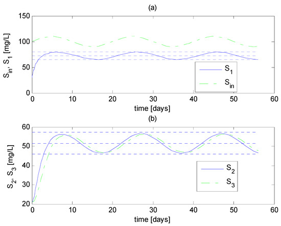
Figure 2. Simulation of the CSTR network model (1)–(4), first case. (a) Time course of $S_1$; the upper and lower horizontal dotted lines indicate the bounds of ${\Omega }_{S1}$. (b) Time course of $S_2$ and $S_3$, the upper and lower horizontal dotted lines indicate the bounds of ${\Omega }_{S2}$, and ${\Omega }_{S3}$.

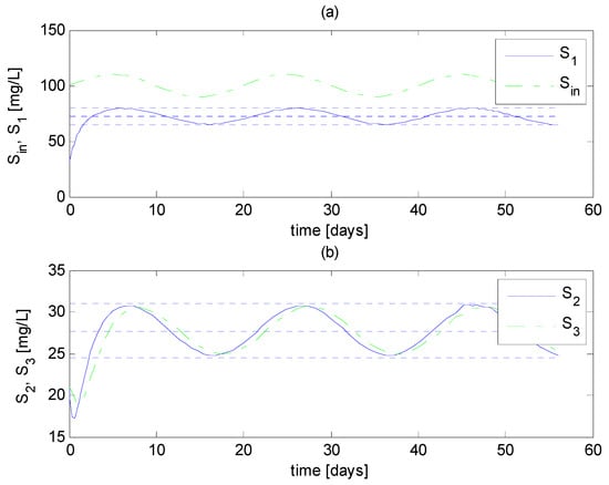
Figure 3. Simulation of the CSTR network model (1)–(4), second case. (a) Time course of $S_1$; the upper and lower horizontal dotted lines indicate the bounds of ${\Omega }_{S1}$. (b) Time course of $S_2$ and $S_3$, the upper and lower horizontal dotted lines indicate the bounds of ${\Omega }_{S2}$ and ${\Omega }_{S3}$.

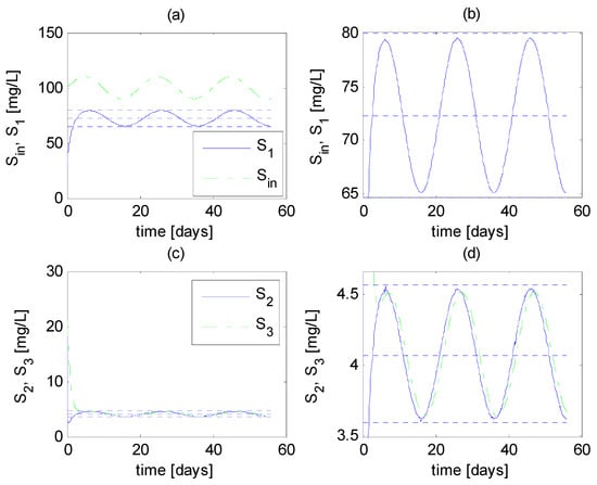
Figure 4. Simulation of the CSTR network model (1)–(4), third case. (a) Time course of $S_1$; the upper and lower horizontal dotted lines indicate the bounds of ${\Omega }_{S1}$. (b) Detail of the time course of $S_1$. (c) Time course of $S_2$ and $S_3$, the upper and lower horizontal dotted lines indicate the bounds of ${\Omega }_{S2}$ and ${\Omega }_{S3}$. (d) Detail of the time course of $S_2$ and $S_3$.

Also, the three simulation cases illustrate the results stated in Theorems 1 and 2: (i) the invariant nature of ${\Omega }_{s1}$, stated in Theorem 1 and discussed in Remark 2: one can see that once S₁ enters ${\Omega }_{s1}$, it remains inside; (ii) the equivalence of the convergence regions ${\Omega }_{s2}$ and ${\Omega }_{s3}$ defined in Theorem 2: one can see that S₂ and S₃ converge to the same regions; (iii) the definitions of ${\Omega }_{s1}$ and ${\Omega }_{s2}$, which indicate that ${\Omega }_{s1}$ and ${\Omega }_{s2}$ can be quite different, as ${\Omega }_{s2}$ depends on the reaction rate r_x2: one can see this remarkable difference in the regions to which S₁ and S₂ converge; (iv) the invariant nature of ${\Omega }_s$, stated in Theorem 2 and discussed in Remark 6: one can see that once the three state variables are inside the convergence region ${\Omega }_s$, that is, $S_1\in {\Omega }_{s1}$, $S_2\in {\Omega }_{s2}$, $S_3\in {\Omega }_{s3}$, simultaneously, they remain inside afterwards.

5. Conclusions

This paper presented the analysis of the stability of a network model comprising three CSTRs with the following features: (i) the pollutant concentration in the inflow of the first CSTR is time varying but bounded; (ii) the first and second CSTRs are connected in series, whereas the second and third CSTRs are connected in parallel with flow exchange; (iii) the states converge to a compact set instead of an equilibrium point. The practical applicability of the arrangement of CSTRs is the creation of a simpler model of pollution removal from wastewater treatment via constructed wetlands, generating a satisfactory description of experimental pollution values with a satisfactory transport dead time.

The convergence sets of the states of the CSTR model were determined, and the global asymptotic convergence to these compact sets and their invariance were proved. Also, the effect of the side tank (third tank) on the transient value of the system states was determined, and it was concluded that it had no effect on the convergence regions. To this end, the proposed stability analysis comprises:

(i)

the definition of a dead-zone Lyapunov-like function for each state, the determination of its properties, and the definition of the overall Lyapunov function as the sum of the dead zone quadratic forms;

(ii)

the determination of the time derivative of the quadratic forms and their properties;

(iii)

the use of these properties in the time derivative of the overall Lyapunov-like function.

References

- Zhou, G.; Liao, X.; Xu, B.; Yu, P.; Chen, G. Simple algebraic necessary and sufficient conditions for Lyapunov stability of a Chen system and their applications. Trans. Inst. Meas. Control 2018, 40, 2200–2210. [Google Scholar] [CrossRef]
- Liao, X.; Zhou, G.; Yang, Q.; Fu, Y.; Chen, G. Constructive proof of Lagrange stability and sufficient—Necessary conditions of Lyapunov stability for Yang–Chen chaotic system. Appl. Math. Comput. 2017, 309, 205–221. [Google Scholar] [CrossRef]
- Zhang, F.; Liao, X.; Zhang, G.; Mu, C. Dynamical Analysis of the Generalized Lorenz Systems. J. Dyn. Control Syst. 2017, 23, 349–362. [Google Scholar] [CrossRef]
- Meng, R.; Chen, S.; Hua, C.; Qian, J.; Sun, J. Disturbance observer-based output feedback control for uncertain QUAVs with input saturation. Neurocomputing 2020, 413, 96–106. [Google Scholar] [CrossRef]
- Boulkroune, A.; M’saad, M.; Farza, M. Adaptive fuzzy system-based variable-structure controller for multivariable nonaffine nonlinear uncertain systems subject to actuator nonlinearities. Neural Comput. Appl. 2017, 28, 3371–3384. [Google Scholar] [CrossRef]
- Zhang, L.; Wang, Z.; Li, S.; Ding, S.; Du, H. Universal finite-time observer based second-order sliding mode control for DC-DC buck converters with only output voltage measurement. J. Franklin Inst. 2020, 357, 11863–11879. [Google Scholar] [CrossRef]
- Shao, X.; Wang, L.; Li, J.; Liu, J. High-order ESO based output feedback dynamic surface control for quadrotors under position constraints and uncertainties. Aerosp. Sci. Technol. 2019, 89, 288–298. [Google Scholar] [CrossRef]
- Askari, M.R.; Shahrokhi, M.; Khajeh Talkhoncheh, M. Observer-based adaptive fuzzy controller for nonlinear systems with unknown control directions and input saturation. Fuzzy Sets Syst. 2017, 314, 24–45. [Google Scholar] [CrossRef]
- Gao, S.; Ning, B.; Dong, H. Fuzzy dynamic surface control for uncertain nonlinear systems under input saturation via truncated adaptation approach. Fuzzy Sets Syst. 2016, 290, 100–117. [Google Scholar] [CrossRef]
- Min, H.; Xu, S.; Ma, Q.; Zhang, B.; Zhang, Z. Composite-Observer-Based Output-Feedback Control for Nonlinear Time-Delay Systems With Input Saturation and Its Application. IEEE Trans. Ind. Electron. 2018, 65, 5856–5863. [Google Scholar] [CrossRef]
- Zhang, F.; Liao, X.; Zhang, G. On the global boundedness of the Lü system. Appl. Math. Comput. 2016, 284, 332–339. [Google Scholar] [CrossRef]
- Slotine, J.-J.E.; Li, W. Applied Nonlinear Control; Prentice Hall: Englewood Cliffs, NJ, USA, 1991; ISBN 0130408905. [Google Scholar]
- Koo, K.-M. Stable adaptive fuzzy controller with time-varying dead-zone. Fuzzy Sets Syst. 2001, 121, 161–168. [Google Scholar] [CrossRef]
- Wang, X.-S.; Su, C.-Y.; Hong, H. Robust adaptive control of a class of nonlinear systems with unknown dead-zone. Automatica 2004, 40, 407–413. [Google Scholar] [CrossRef]
- Su, C.-Y.; Feng, Y.; Hong, H.; Chen, X. Adaptive control of system involving complex hysteretic nonlinearities: A generalised Prandtl–Ishlinskii modelling approach. Int. J. Control 2009, 82, 1786–1793. [Google Scholar] [CrossRef]
- Ranjbar, E.; Yaghubi, M.; Abolfazl Suratgar, A. Robust adaptive sliding mode control of a MEMS tunable capacitor based on dead-zone method. Automatika 2020, 61, 587–601. [Google Scholar] [CrossRef]
- Rincón, A.; Hoyos, F.E.; Candelo-Becerra, J.E. Adaptive Control for a Biological Process under Input Saturation and Unknown Control Gain via Dead Zone Lyapunov Functions. Appl. Sci. 2021, 11, 251. [Google Scholar] [CrossRef]
- Rincón, A.; Piarpuzán, D.; Angulo, F. A new adaptive controller for bio-reactors with unknown kinetics and biomass concentration: Guarantees for the boundedness and convergence properties. Math. Comput. Simul. 2015, 112, 1–13. [Google Scholar] [CrossRef]
- Rincón, A.; Florez, G.Y.; Olivar, G. Convergence Assessment of the Trajectories of a Bioreaction System by Using Asymmetric Truncated Vertex Functions. Symmetry 2020, 12, 513. [Google Scholar] [CrossRef]
- Meadows, T.; Weedermann, M.; Wolkowicz, G.S.K. Global Analysis of a Simplified Model of Anaerobic Digestion and a New Result for the Chemostat. SIAM J. Appl. Math. 2019, 79, 668–689. [Google Scholar] [CrossRef]
- Mairet, F.; Ramírez, C.H.; Rojas-Palma, A. Modeling and stability analysis of a microalgal pond with nitrification. Appl. Math. Model. 2017, 51, 448–468. [Google Scholar] [CrossRef]
- Sari, T.; Mazenc, F. Global dynamics of the chemostat with different removal rates and variable yields. Math. Biosci. Eng. 2011, 8, 827–840. [Google Scholar] [CrossRef] [PubMed]
- Almeida, R.; Hristova, S.; Dashkovskiy, S. Uniform bounded input bounded output stability of fractional-order delay nonlinear systems with input. Int. J. Robust Nonlinear Control 2021, 31, 225–249. [Google Scholar] [CrossRef]
- Garrido, H.; Curadelli, O.; Ambrosini, D. On the assumed inherent stability of semi-active control systems. Eng. Struct. 2018, 159, 286–298. [Google Scholar] [CrossRef]
- Vafamand, N.; Asemani, M.H.; Khayatian, A. Robust L1 Observer-Based Non-PDC Controller Design for Persistent Bounded Disturbed TS Fuzzy Systems. IEEE Trans. Fuzzy Syst. 2018, 26, 1401–1413. [Google Scholar] [CrossRef]
- Kong, L.; He, W.; Dong, Y.; Cheng, L.; Yang, C.; Li, Z. Asymmetric Bounded Neural Control for an Uncertain Robot by State Feedback and Output Feedback. IEEE Trans. Syst. Man Cybern. Syst. 2019, 1–12. [Google Scholar] [CrossRef]
- Yu, J.; Zhao, L.; Yu, H.; Lin, C. Barrier Lyapunov functions-based command filtered output feedback control for full-state constrained nonlinear systems. Automatica 2019, 105, 71–79. [Google Scholar] [CrossRef]
- Niu, B.; Liu, Y.; Zhou, W.; Li, H.; Duan, P.; Li, J. Multiple Lyapunov Functions for Adaptive Neural Tracking Control of Switched Nonlinear Nonlower-Triangular Systems. IEEE Trans. Cybern. 2020, 50, 1877–1886. [Google Scholar] [CrossRef] [PubMed]
- De Battista, H.; Jamilis, M.; Garelli, F.; Picó, J. Global stabilisation of continuous bioreactors: Tools for analysis and design of feeding laws. Automatica 2018, 89, 340–348. [Google Scholar] [CrossRef]
- El Hajji, M.; Chorfi, N.; Jleli, M. Mathematical modeling and analysis for a three-tiered microbial food web in a chemostat. Electron. J. Differ. Equ. 2017, 2017, 1–13. [Google Scholar]
- Marsili-Libelli, S.; Checchi, N. Identification of dynamic models for horizontal subsurface constructed wetlands. Ecol. Modell. 2005, 187, 201–218. [Google Scholar] [CrossRef]
- Langergraber, G. Applying Process-Based Models for Subsurface Flow Treatment Wetlands: Recent Developments and Challenges. Water 2016, 9, 5. [Google Scholar] [CrossRef]
- Defo, C.; Kaur, R.; Bharadwaj, A.; Lal, K.; Kumar, P. Modelling approaches for simulating wetland pollutant dynamics. Crit. Rev. Environ. Sci. Technol. 2017, 47, 1371–1408. [Google Scholar] [CrossRef]
- Davies, L.C.; Vacas, A.; Novais, J.M.; Freire, F.G.; Martins-Dias, S. Vertical flow constructed wetland for textile effluent treatment. Water Sci. Technol. 2007, 55, 127–134. [Google Scholar] [CrossRef] [PubMed][Green Version]
- Freire, F.G.; Davies, L.C.; Vacas, A.M.; Novais, J.M.; Martins-Dias, S. Influence of operating conditions on the degradation kinetics of an azo-dye in a vertical flow constructed wetland using a simple mechanistic model. Ecol. Eng. 2009, 35, 1379–1386. [Google Scholar] [CrossRef]
- Ioannou, P.A.; Sun, J. Robust Adaptive Control; Prentice Hall: Upper Saddle River, NJ, USA, 1996; ISBN 9780486498171. [Google Scholar]
- García-Ávila, F.; Patiño-Chávez, J.; Zhinín-Chimbo, F.; Donoso-Moscoso, S.; Flores del Pino, L.; Avilés-Añazco, A. Performance of Phragmites Australis and Cyperus Papyrus in the treatment of municipal wastewater by vertical flow subsurface constructed wetlands. Int. Soil Water Conserv. Res. 2019, 7, 286–296. [Google Scholar] [CrossRef]
Publisher’s Note: MDPI stays neutral with regard to jurisdictional claims in published maps and institutional affiliations. |
© 2021 by the authors. Licensee MDPI, Basel, Switzerland. This article is an open access article distributed under the terms and conditions of the Creative Commons Attribution (CC BY) license (https://creativecommons.org/licenses/by/4.0/).