SVM-Based Bearing Anomaly Identification with Self-Tuning Network-Fuzzy Robust Proportional Multi Integral and Smart Autoregressive Model

Featured Application

Condition monitoring and fault diagnosis.

Abstract

In this paper, the combination of an indirect self-tuning observer, smart signal modeling, and machine learning-based classification is proposed for rolling element bearing (REB) anomaly identification. The proposed scheme has three main stages. In the first stage, the original signal is resampled, and the root mean square (RMS) signal is extracted from it. In the second stage, the normal resampled RMS signal is approximated using the AutoRegressive with eXternal Uncertainty (ARXU) technique. Moreover, the nonlinearity of the bearing signal is solved using the combination of the ARXU and the machine learning-based regression, which is called AMRXU. After signal modeling by AMRXU, the RMS resampled signal is estimated using a combination of the proportional multi-integral (PMI) technique, the variable structure (VS) Lyapunov technique, and a self-tuning network-fuzzy system (SNFS). Finally, in the third stage, the difference between the original signal and the estimated one is calculated to generate the residual signal. A machine learning-based classification technique is utilized to classify the residual signal. The Case Western Reserve University (CWRU) dataset is used to evaluate anomaly identification performance of the proposed scheme. Regarding the experimental results, the average accuracy for REB crack identification is 98.65%, 97.7%, 97.35%, and 97.67%, respectively, when the motor torque loads are 0-hp, 1-hp, 2-hp, and 3-hp.

1. Introduction

One of the principal mechanical components in global industries is the rotating machine. With the rapid and daily advancements in technology, new rotating machinery tools appear that are better, more complicated, and more accurate. Therefore, their functionality affects safety and operational stability and reliable industrial production. However, due to the complexity in rotary machinery systems and the multiplicity of parts, the probability of failure is greatly increased. Among all the components in rotating machines, rolling element bearings (REBs) are used in a majority of them. Bearings facilitate the movement of components owing to the rolling action and diminished friction. Their exceptional anti-friction ability makes them a very important tool wherever there is the challenge of energy savings [1].

Among all the industrial attention, one absolute concern to ensure reliability and safety in advanced technical systems is anomaly detection. Timely and correct anomaly detection prevents disastrous events and increases production efficiency. Furthermore, immediate fault diagnosis in REBs can help to figure out the main reasons for product corruption and can avoid irregularities in the system and/or complete failure [2].

Even though fault detection and diagnosis are acutely challenging and intricate due to nonlinear parameters in the bearings and in work complexity, bearings are one of the critical components that can cause 40 to 50% of all failures in rotating machines [3,4]. Accordingly, fault diagnosis for these elements is a necessity.

Within this concept, a maintenance procedure for monitoring the health situation of machinery is necessary, which makes the optimal decision to prevent or reduce faults mainly based on condition monitoring information. According to [4,5], for an efficient machinery health diagnosis program, one of the principal technical processes is data acquisition.

Numerous sensors are applied over a certain time to find industrial irregularities (for example, in bearings) based on physical signals called time-series signals [6,7]. A time series mainly operates as input data with which to train models for industrial anomaly detection [2,8]. Motivated by the discourse above, the issue of condition-monitoring procedures becomes important for identifying serious changes that are expressive of a fault.

Therefore, a multitude of studies have been conducted to monitor the condition of bearings [9,10,11,12,13]. Subsequently, different methods have been determined for condition monitoring in order to recognize and classify bearing faults. These methods are defined based on vibration signals, acoustic emission signals, and motor current signature analysis [14,15].

Generally speaking, faults in bearings can be classified as follows: (i) the outer bearing race fault (OURF), (ii) the inner bearing race fault (INRF), (iii) the roller fault (ROLF), and (iv) the cage fault [15,16]. To recognize, discover, and classify faults in rolling element bearings, vibration supervising is widely used and is an economical monitoring method. Nowadays, fundamental monitoring of rolling element bearings generally depends on analyzing vibration signals due to their great capabilities in describing REB performance [11]. Bearings generate vibration, either due to differing compliance or from the appearance of a crack. Numerous studies have been carried out on vibration signal analysis, and a variety of research has been conducted based on the kinds of defects and fault diagnosis techniques [8,17,18].

Based on the information provided, fault diagnosis in bearings is conducted with various methods. The manner of signal processing can be leveraged as a known procedure; other methods exist that lean on data-driven techniques and model-based techniques; finally, one further method is an amalgamation of the above techniques—the hybrid method [11,19,20]. What drives us to use the hybrid method is that these other methods have weaknesses that make them difficult to use. For instance, there are several challenges for signal-based techniques under an unknown status [19]. Moreover, data-driven techniques have limitations related to massive datasets, while model-based approaches have difficulties in modeling a system accurately [18,19,20]. The more robust and accurate fault diagnostics process should be considered if an uncertain situation exists [11]. To overcome the mentioned limitations and attain a more effective technique for flaw diagnosis, the hybrid method is proposed. A combination of the model-based approach, data-driven method, and signal-based approach is proposed in which diagnosis results are claimed to be less complicated, more reliable, and accurate [11]. Some examples are as follows: the combination of signal processing and deep learning techniques has been proposed in [21]. This research has two main stages. First, the hybrid feature pool was generated using envelope spectrum, time domain and wavelet packet transform. Next, the stacked autoencoder was suggested to perform fault detection and diagnosis. In this work, determining the number of features and selecting the best features are the main challenges. The combination of data-driven and modern control algorithms for fault detection and diagnosis has been presented in [22]. In this research, the second order system was modeled using the linear AutoRegressive with eXternal input (ARX)-Laguerre technique. The proportional integral (PI) observer was evaluated for the signal estimation. This technique is linear; however, for nonlinear and non-stationary signals such as vibration bearing signals, the accuracy may decrease. The combination of the modern control algorithm and deep learning approach has been proposed in [23]. In this research, the rotor signal was modeled using the ARX-Laguerre technique. The combination of the PI observer and the scalable deep neural network was also used for signal estimation and fault decision. In this work, the combination of the signal-based approach for signal modeling and artificial intelligence approaches for signal estimation, and a machine learning method for classification is recommended as a hybrid algorithm for fault diagnosis of bearing.

Even though the current and voltage encompass all the information, sometimes fitting raw signals into some groups of rules and criteria for interpreting the fundamental messages that come from the signals is very difficult. This is where feature extraction methods help to dig out beneficial information purposefully from within the considered system. Using proper feature extraction techniques, researchers can obtain further knowledge on fault classification, which enables them to provide more efficient methods for this topic [21,24].

Signal modeling is one of the critical challenges to design the modern control-based approach for fault diagnosis [25]. The challenge in nonlinear and nonstationary signal modeling was recently discussed [23,26,27,28,29]. Signal modeling can be categorized into two standard groups: modeling based on the system’s dynamics [29], and data-driven modeling [18,22,30]. The challenge of vibration signal modeling may be solved by the mathematical-based approach and five degrees of freedom vibration bearing modeling are included [29]. In complex systems, modeling with the dynamics-based approach has the challenge of intricacy.

To reduce the challenge from complexity in dynamics-based system modeling, data-driven signal modeling such as linear regression with ordinary least squares, AutoRegressive models (AR), the AutoRegressive with eXternal input (ARX) model, random forest, ARX-Laguerre, multivariate adaptive regression splines, support vector regression, the neural network, and Gaussian process regression have been suggested [31]. Specially, in [22,30] the ARX and ARX-Laguerre methods have been used for signal modeling in second order systems. However, the accuracy of the nonlinear and nonstationary signal approximation is not good, which is the main challenge of these techniques [22,23,30].

To estimate the original signals, diverse algorithms have been suggested in recent years. The observation-based technique is one of the powerful mechanisms for signal estimation [25]. Artificial Intelligence (AI)-based observers and modern control-based observers are two main groups for signal estimation [19,20]. AI-based observers, such as the fuzzy logic observer [20], the neural network observer [21], and the neuro-fuzzy observer [22], have the same challenge (namely, reliability). Modern control-based observers (including linear-based observers and nonlinear-based observers) have been used for signal estimations [18,19,32]. The sliding mode observer is one of the most robust and reliable estimators for fault diagnosis. The application of the sliding mode observer for fault diagnosis was presented in [18]. Despite its stability, reliability, and robustness, the sliding mode observer suffers from complexity and the chattering phenomenon. The next nonlinear-based observer is the feedback linearization approach [33]. However, this approach solves the issue of the chattering phenomenon; robustness and reliability are two important drawbacks. Thus, the main challenge of nonlinear modern control-based observers (such as the sliding mode observer and the feedback linearization observer) is complexity. To reduce complexity, modern linear control-based observers, such as the proportional integral (PI) observer [22] and the proportional multi-integral (PMI) observer [34], have been suggested. Although PI observers and PMI observers have good performance in terms of accuracy and complexity, they have some problems related to robustness about uncertainties [34]. To address the robustness issue, a combination of PMI observer and sliding mode approach was used in [34]. The main limitation of this algorithm is to increase the amount of chattering and signal fluctuations in the presence of variation in torque load and motor speed.

To fault and state condition classifications, diverse classification algorithms such as decision trees [35], nearest neighbor classifiers [36], support vector machines [37], and ensemble classifiers have been introduced.

In the paper, the hybrid-based fault diagnosis approach is suggested for anomaly identification of the bearing. The proposed hybrid-based approach has three main steps: (i) preprocessing and feature extraction step, (ii) signal modeling and estimation step, and (iii) classification step. Based on the above, the feature extraction technique is considered as the first stage. In this research, the main stage for designing the hybrid technique for rolling element bearing crack identification is to compute residual signals, which are calculated based on the difference between original signals and estimated signals. Modeling is also the main critical challenge in modern control-based observers for signal estimation. Subsequently, the first step in estimating a signal using observers is signal modeling to approximate the state-space function of the signal. Therefore, in the paper, we apply machine learning-based regression (MBR) to the ARX with uncertainty input (ARXU) technique for signal approximation, which is called “AMRXU”. After signal modeling, the original signals are estimated before computing the residual signals. To do this, first, the PMI observer is recommended. After that, to address the robustness limitation in the PMI, the variable structure (VS)-Lyapunov is adopted. Apart from reducing the complexity and increasing the accuracy and robustness of this technique, the flexibility about uncertainties in various torque loads, motor speeds, or crack sizes can be a weakness. To overcome this issue, we use the self-tuning hybrid-based observer which is a combination of a self-tuning AI-based technique and modern control-based approach to improve the positive points, which is called “AVSPMI”. Next, the residual signals are computed using the difference between the original signals and the estimated ones. Regarding the accuracy and robustness of the estimation of the signal, the residual signal levels are different in dissimilar classes. Finally, we select the SVM technique for classification. The contributions of this paper can be summarized as follows:

• Indirect signal modeling by extracting the state-space nonlinear function using the combination of machine learning-based regression and ARXU technique.
• Indirect signal estimation by using the combination of the PI observer, extended integral term, VS-Lyapunov technique, and self-tuning network-fuzzy system.
• Combination of AMRXU, AVSPMI, and SVM-based approaches for bearing fault detection and classification.

The remainder of this paper is organized as the follows: The proposed Scheme is briefly described, and the block diagram of the proposed scheme has been shown in Section 2. The data acquisition from the Case Western Reverse University (CWRU) dataset is described in Section 3. Next, the preprocessing is explained in the Section 4. In Section 5, first, a smart autoregressive signal modeling is proposed over normal signal modeling. Next, a self-tuning hybrid-based observer is designed for signal estimation in normal conditions. The signal condition is classified by machine learning-based classifier in Section 6. The experimental results are presented in Section 7, and the conclusion is presented in Section 8.

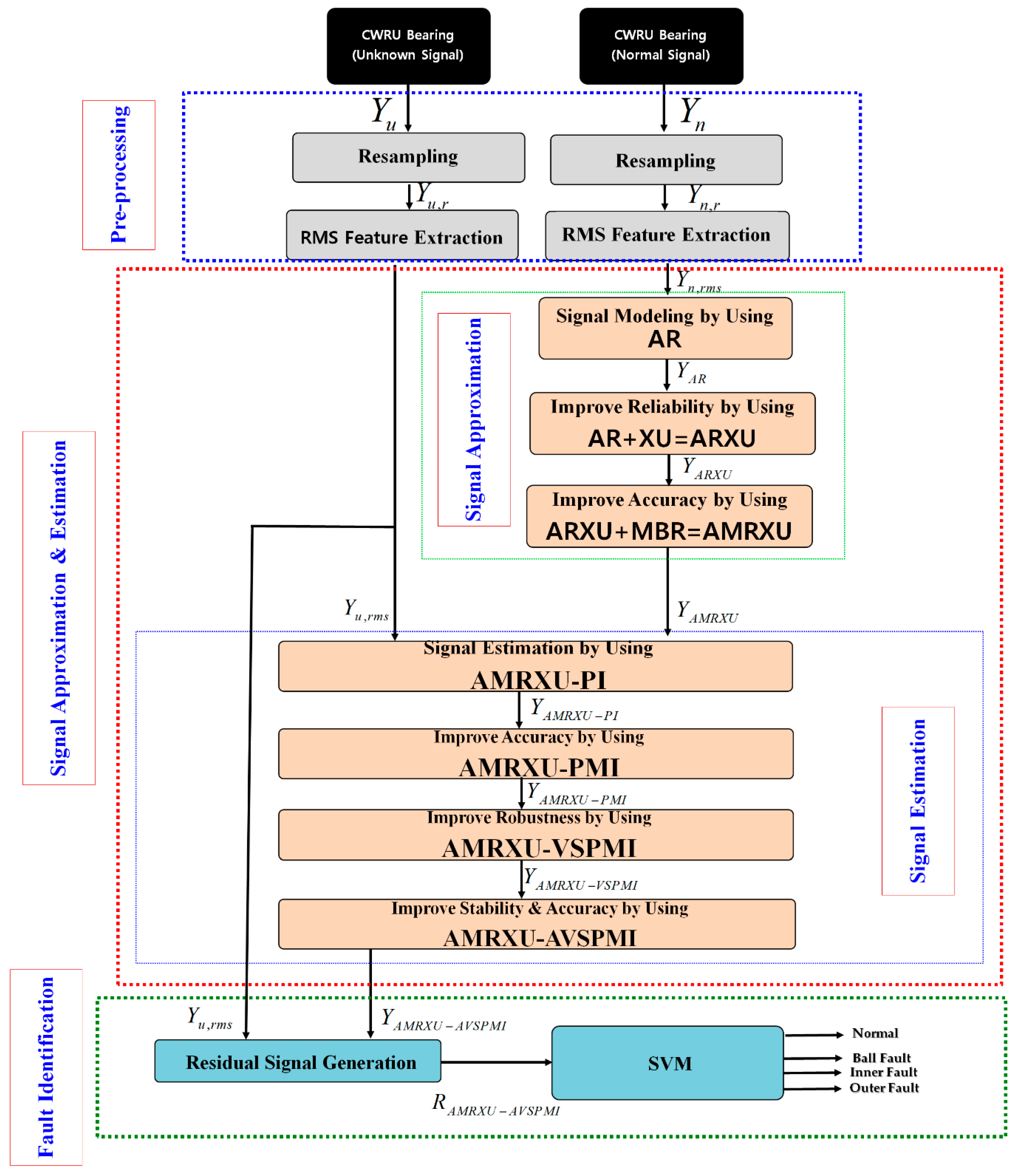
2. Proposed Scheme and Block Diagram

Figure 1 shows the overall block diagram of the proposed scheme, which consists of three main stages: the preprocessing stage, signal approximation and estimation stage, and fault identification stage.

At first, in the preprocessing stage, the vibration signals are resampled, and next, the RMS features are extracted from the resampled signals. The second stage is used to model and estimate the resampled RMS signals. Based on the difference between estimated signals and original ones, the signals can be classified into different conditions.

Thus, to estimate the resampled RMS signal, a modern control-based observation method is suggested. To build a modern control-based observer, first, the resampled RMS signal in normal condition needs to be modeled. So, the first step in the second stage is signal modeling. The combination of AR, external uncertainties inputs (XU), and MBR, which is denoted as AMRXU in the paper, is suggested for normal resampled RMS signal modeling. More specifically, the AR technique is used for normal signal modeling. To increase the robustness and accuracy, the AR technique is combined with the XU technique to implement the ARXU method for modeling the resampled RMS signal in the healthy state. This signal is nonlinear and nonstationary. Subsequently, to increase the accuracy of signal modeling with the property of nonlinearity and nonstationary, the resampled RMS signal in the normal condition is modeled with a combination of the ARXU and the MBR, which is denoted as AMRXU.

After modeling the resampled RMS signal in the normal condition, the indirect self-tuning observer, which is a combination of the modern control-based observer and AI-based approach, has been designed. Thus, first, the PI observer is implemented when the signal is modeled by the AMRXU technique (henceforth called AMRXU-PI). After that, to improve the accuracy, the AMRXU-PI observer is combined with integral term (I), which is called the AMRXU-PMI observer. Moreover, to increase the robustness in uncertain conditions (e.g., variant motor torque loads and variant bearing crack sizes) the AMRXU-PMI is combined with a VS-Lyapunov scheme, which is denoted as the AMRXU-VSPMI method. Next, the indirect self-tuning observer is designed by using the combination of the AMRXU-VSPMI with the self-tuning network-fuzzy system (SNFS) technique, which is denoted as AMRXU-AVSPMI. After estimating the resampled RMS signals using the proposed AMRXU-AVSPMI method, in the third stage, the machine learning technique is used for fault classification. To do this, first, the residual signals are computed using the difference between the original and estimated signal. Next, the support vector machine (SVM) is used for classification such that the residual signals will be classified into four main groups: normal (NORM), ROLF, INRF, and OURF.

3. Dataset

A CWRU dataset was selected to test the recommended scheme. In this work, a two-horsepower (hp) induction motor was selected to power the rolling bearings (6205-2RS JEM from SKF, Gothenburg, Sweden) at various rotational speeds. Moreover, a vibration sensor with a 48 kHz sampling rate was used for data collection. This dataset has four classes: NORM, ROLF, INRF, and OURF. Moreover, three different crack sizes are included (0.007 inches, 0.014 inches, and 0.021 inches) and the data were recorded at 0-hp, 1-hp, 2-hp, and 3-hp torque loads [38].

Table 1. Case Western Reserve University Vibration Dataset classes, torque loads, and crack sizes [38].

Class	Torque Load (hp)	Crack Sizes (Inches)
NORM	0, 1, 2, 3	-
ROLF	0, 1, 2, 3	0.007, 0.014, 0.021
INRF	0, 1, 2, 3	0.007, 0.014, 0.021
OURF	0, 1, 2, 3	0.007, 0.014, 0.021

lists the CWRU data descriptions for healthy and defective states.

4. Preprocessing

The proposed scheme has three main sections: (a) preprocessing, (b) resampled signal approximation and estimation, and (c) fault detection and diagnosis. To calculate signal conditions and the probable types of fault by using an intelligence-based indirect observer and a machine-learning approach, it may be necessary to calculate one or more statistical features extracted from the bearing signal. Therefore, in order to extract appropriate features, the bearing raw signal is first windowed at exactly the same size. Based on [38], the range of rotational speeds in the CWRU dataset is 1730 to 1797 revolutions per minute (RPM) or 28 to 30 revolutions per second (RPS). In addition, the data collection sampling rate frequency for the CWRU dataset is 48 kHz. So, to cover the bearing conditions, 1200 samples are needed every rotation. Moreover, because the signal length is 120,000 samples, we have 100 windows for each condition. In the next step, the RMS signal is selected as a feature based on the following definition [12]:

$$Y_{rms}=\sqrt{\frac{1}{N}{\displaystyle \sum }_{i=1}^N{Y}^2}$$

(1)

Here, $Y_{rms}, N$, and $Y$ denote the resampled RMS value for each window, the number of windows calculated (based on the resampling technique), and the original bearing signal in each window resampled using the above technique, respectively.

5. Signal Approximation and Estimation

As seen in Figure 1, the proposed scheme has three main sections: (a) preprocessing, (b) resampled signal approximation and estimation, and (c) fault classification. Preprocessing was explained in the previous section. In the second section, resampled RMS signals are approximated and estimated under two main subsections: (i) modeling the normal resampled RMS signal and (ii) estimating the resampled RMS signals under normal and abnormal conditions. The following steps are used for signal modeling: an AR design for resampled RMS normal signal modeling, improvement of the robustness and performance from the AR technique using defined uncertainty as an external input that is ARXU technique, (i.e., ARXU), and solving nonlinear bearing signal behavior using the combination of MBR and ARXU to design AMRXU.

5.1. Combination of ARXU and MBR for Signal Approximation

After resampling and extracting the RMS feature from the original healthy signal, the AR technique models and extracts the state-space equation from the RMS signal under normal conditions. The state-space definition of a healthy signal based on the AR technique is represented using the following equations [39]:

$$X_{AR}\left(k+1\right)={\mathit{\ell }}_X{X}_{AR}\left(k\right)+{\mathit{\ell }}_e{e}_{AR}\left(k\right)$$

(2)

$$Y_{AR}\left(k\right)={\mathit{\ell }}_Y{}^T{X}_{AR}\left(k\right)$$

(3)

$$e_{AR}\left(k\right)=Y_{n,rms}\left(k\right)-Y_{AR}\left(k-1\right)$$

(4)

Here, $X_{AR}\left(k\right), Y_{AR}\left(k\right),$ and $\left({\mathit{\ell }}_X,{\mathit{\ell }}_Y,{\mathit{\ell }}_e\right)$, respectively, are the state of RMS signal modeling using the AR technique, the output of RMS signal modeling using the AR technique, and the state-space tuning coefficients based on the AR algorithm. The AR algorithm for modeling the signal is valuable for the time-series signal. To improve the robustness and performance against uncertainties, an ARXU is recommended. The mathematical definition of ARXU is represented as the following equations [39,40]:

$$X_{ARXU}\left(k+1\right)=\left[{\mathit{\ell }}_X{X}_{ARXU}\left(k\right)+{\mathit{\ell }}_{\epsilon }{\mathrm{\epsilon }}_{ARXU}\left(k\right)\right]+{\mathit{\ell }}_e{e}_{ARXU}\left(k\right)$$

(5)

$$Y_{ARXU}\left(k\right)={\mathit{\ell }}_Y{}^T{X}_{ARXU}\left(k\right)$$

(6)

$$e_{ARXU}\left(k\right)=Y_{n,rms}\left(k\right)-Y_{ARXU}\left(k-1\right),$$

(7)

$${\mathrm{\epsilon }}_{ARXU}\left(k\right)=Y_{ARXU}\left(k\right)-Y_{n,rms}\left(k\right)$$

(8)

Here, $X_{ARXU}\left(k\right), Y_{ARXU}\left(k\right),{\mathrm{\epsilon }}_{ARXU}\left(k\right), Y_{n,rms}\left(k\right),$ and $\left({\mathit{\ell }}_{\epsilon }\right)$, respectively, are the state of RMS signal modeling using ARXU, the output of the RMS signal modeling using ARXU, the uncertainties effect estimation and feedback as inputs to reduce the effect of uncertainties using ARXU, the original RMS signal for a healthy condition, and the state-space tuning coefficient based on the ARXU algorithm.

The main obstacle in time-series signal modeling is estimating nonlinear behavior. Nonlinear behavior modeling of bearings is complicated. To address this issue, MBR is recommended [41,42]. MBR is a learning technique to approximate the resampled RMS signal in a normal state. Therefore, the combination of ARXU and MBR is introduced in this research. The basic concept of the MBR technique is the learning method. The following function represents the mathematical definition of MBR [42]:

$${\mathit{\hslash }}_{MBR}={\displaystyle \sum }_i\left({\partial }_i{}^{+}-{\partial }_i{}^{-}\right)\varkappa ({\theta }_i,\theta )+\mathsf{\Theta }.$$

(9)

Here, ${\mathit{\hslash }}_{MBR},\left({\partial }_i{}^{+},{\partial }_i{}^{-}\right),\varkappa \left({\theta }_i,\theta \right),$ and $\mathsf{\Theta }$ are the output-modeled RMS resampled normal signal based on MBR, the Lagrange coefficients, the kernel, and the bias, respectively. Various kernel functions have been introduced in research papers; in this work, the Gaussian function is selected and represented as follows:

$$\varkappa \left({\theta }_i,\theta \right)=e^{\left(-\frac{1}{2{\sigma }^2}\parallel {\theta }_i-\theta {\parallel }^2\right)}.$$

(10)

Here, $\sigma$ is variance. Moreover, the minimum value for $\left({\partial }_i{}^{+},{\partial }_i{}^{-}\right)$ can be calculated based on the following equation:

$$\min {\displaystyle \sum }_i{\displaystyle \sum }_j\left({\partial }_i{}^{+}-{\partial }_i{}^{-}\right)\left({\partial }_j{}^{+}-{\partial }_j{}^{-}\right)\varkappa \left({\theta }_i,\theta \right).$$

(11)

If $\varkappa \left({\theta }_i,\theta \right)$ is defined as ${ℳ}_{ij}$ and is based on Equation (11), then

$$\min {\displaystyle \sum }_i{\displaystyle \sum }_j\left({\partial }_i{}^{+}.{\partial }_j{}^{+}\right){ℳ}_{ij}-\left({\partial }_i{}^{-}.{\partial }_j{}^{+}\right){ℳ}_{ij}-\left({\partial }_i{}^{+}.{\partial }_j{}^{-}\right){ℳ}_{ij}+\left({\partial }_i{}^{-}.{\partial }_j{}^{-}\right){ℳ}_{ij}.$$

(12)

Moreover, if $ℳ=\left[{ℳ}_{ij}\right]\in {\mathrm{ℝ}}^{n\times n}, \partial ={\left[\begin{array}{c}{\partial }^{+}\\ {\partial }^{-}\end{array}\right]}_{2n\times 1}, \mathrm{and}$ $\mathit{\aleph }=\left[\begin{array}{cc}ℳ& -ℳ\\ -ℳ& ℳ\end{array}\right]$, then Equation (12) is rewritten as:

$$min\frac{1}{2}{\partial }^T\mathit{\aleph }\partial +{\mathit{ℒ}}^T\partial .$$

(13)

Here, $\mathit{ℒ}={\left[\begin{array}{c}-Y+\beta \\ Y+\beta \end{array}\right]}_{2n\times 1}$, in which $Y$ and $\beta$ are the resampled RMS signal under normal conditions, and the boundary of acceptable signal modeling, respectively. In addition, bias is determined using the following function:

$$\mathsf{\Theta }=\frac{1}{s}{\displaystyle \sum }_{s\in S}\left[Y_s-{\displaystyle \sum }_{i\in S}\left({\partial }_i{}^{+}-{\partial }_i{}^{-}\right)\times \varkappa ({\theta }_i,{\theta }_s)-\beta \times sgn\left({\partial }_i{}^{+}-{\partial }_i{}^{-}\right)\right].$$

(14)

Here, $Y_s$ and $S$ denote the support vector resampled RMS signal in a normal condition, and the support vector, respectively. The support vector is defined as

$$S=\left\{i|0\le {\partial }_i{}^{+}-{\partial }_i{}^{-}\le \Delta \right\}.$$

(15)

Here, $\Delta$ is a constant. So, the combination of the ARXU and MBR algorithms (or AMRXU) is represented with the following definitions:

$$X_{AMRXU}\left(k+1\right)=\left[{\mathit{\ell }}_X{X}_{AMRXU}\left(k\right)+{\mathit{\ell }}_{\mathrm{\epsilon }}{\mathrm{\epsilon }}_{AMRXU}\left(k\right)+{\mathit{\ell }}_{MBR}{\mathit{\hslash }}_{MBR}\right]+{\mathit{\ell }}_e{e}_{AMRXU}\left(k\right),$$

(16)

$$Y_{AMRXU}\left(k\right)={\mathit{\ell }}_Y{}^T{X}_{AMRXU}\left(k\right),$$

(17)

$$e_{AMRXU}\left(k\right)=Y_{n,rms}\left(k\right)-Y_{AMRXU}\left(k-1\right),$$

(18)

$${\mathrm{\epsilon }}_{AMRXU}\left(k\right)=Y_{AMRXU}\left(k\right)-Y_{n,rms}\left(k\right).$$

(19)

Here, $X_{AMRXU}\left(k\right), Y_{AMRXU}\left(k\right),{\mathrm{\epsilon }}_{AMRXU},$ and ${\mathit{\ell }}_{MBR}$, respectively, are the state of RMS signal modeling using AMRXU, the output of RMS signal modeling using AMRXU, the uncertainties-effect estimation and feedback as inputs to reduce the effect of uncertainties of using AMRXU, and the state-space tuning coefficient.

5.2. Combination of AMRXU-PMI Observer, VS-Lyapunov Algorithm, and SNFS Technique for Resampled RMS Signal Estimation

According to Figure 1, after modeling the signal and extracting the nonlinear state-space equation from the resampled RMS signal in a healthy condition, normal and abnormal resampled RMS signals are estimated using the proposed self-tuning hybrid-based scheme. Although the accuracy of resampled RMS normal signal modeling using AMRXU is 98.5%, for abnormal resampled RMS signals (and for normal resampled RMS signals under torque loads of 1 hp, 2 hp, and 3 hp), accuracy in signal modeling decreases. So, the signal estimation technique is suggested in this work. The proposed algorithm is used to estimate the resampled RMS signal using the following steps. First, the resampled RMS signals are estimated using the AMRXU-PI observer, and its mathematical state-space equations are extracted. In the second step, to improve the accuracy of the AMRXU-PI observer, combining the integral term and the AMRXU-PI observer designs the AMRXU-PMI observer. Third, to increase the effect of robustness in the AMRXU-PMI observation technique, the VS-Lyapunov algorithm is used alongside the AMRXU-PMI observer, making the AMRXU-VSPMI observer. In the last step, to improve accuracy and flexibility in uncertain situations, an intelligent technique based on the SNFS is used along with AMRXU-VSPMI, which builds the proposed method: the AMRXU-AVSPMI observer. Thus, the state-space equations for the AMRXU-PI observer are as follows:

$$\begin{array}{cc}\hfill X_{AMRXU-PI}\left(k+1\right)& =\left[{\mathit{\ell }}_X{X}_{AMRXU-PI}\left(k\right)+{\mathit{\ell }}_{\mathrm{\epsilon }}{\mathrm{\epsilon }}_{AMRXU-PI}\left(k\right)+{\mathit{\ell }}_{MBR}{\mathit{\hslash }}_{MBR}\right]\hfill \\ & +{\mathit{\ell }}_e{e}_{AMRXU-PI}\left(k\right)+{\mathrm{\epsilon }}_{AMRXU-PI}+{\mathit{\ell }}_p\left(Y_{AMRXU-PI}\left(k\right)-Y_{AMRXU}\left(k\right)\right),\hfill \end{array}$$

(20)

$$Y_{AMRXU-PI}\left(k\right)={\mathit{\ell }}_Y{}^T{X}_{AMRXU-PI}\left(k\right),$$

(21)

$$e_{AMRXU-PI}\left(k\right)=Y_{u,rms}\left(k\right)-Y_{AMRXU-PI}\left(k-1\right),$$

(22)

$${\mathrm{\epsilon }}_{AMRXU-PI}\left(k+1\right)={\mathrm{\epsilon }}_{AMRXU-PI}\left(k\right)+{\mathit{\ell }}_{i\left(1\right)}\left({\mathrm{\epsilon }}_{AMRXU-PI}\left(k\right)-{\mathrm{\epsilon }}_{AMRXU}\left(k\right)\right).$$

(23)

Here, $X_{AMRXU-PI}\left(k\right), Y_{AMRXU-PI}\left(k\right),e_{AMRXU-PI}\left(k\right), {\mathrm{\epsilon }}_{AMRXU-PI}, Y_{u,rms}\left(k\right)$, and $\left({\mathit{\ell }}_p,{\mathit{\ell }}_{i\left(1\right)}\right)$, respectively, are the state estimation of RMS signal modeling, the output estimation of RMS signal modeling, the estimation error, and the uncertainties estimation (all using the AMRXU-PI observation technique), the unknown resampled RMS signals, and the state-space tuning coefficients for proportional and integral terms, also based on the AMRXU-PI observation algorithm. Based on Equation (20), the proportional term is used to increase the accuracy in state estimation of the RMS signal modeling. Moreover, based on Equation (23), the integral term is selected to reduce the effect of uncertainties in signal estimation. To improve the accuracy of the AMRXU-PI observer, the AMRXU-PMI observer is recommended here. Therefore, based on Figure 1, to estimate the resampled RMS signal for healthy and faulty conditions, and to improve the accuracy of the AMRXU-PI observer, in the second step, the AMRXU-PMI observer is selected, and the state-space equations are as follows:

$$\begin{array}{cc}\hfill X_{AMRXU-PMI}\left(k+1\right)& = \left[{\mathit{\ell }}_X{X}_{AMRXU-PMI}\left(k\right)+{\mathit{\ell }}_{\mathrm{\epsilon }}{\mathrm{\epsilon }}_{AMRXU-PMI}\left(k\right)+{\mathit{\ell }}_{MBR}{\mathit{\hslash }}_{MBR}\right]\hfill \\ & +{\mathit{\ell }}_e{e}_{AMRXU-PMI}\left(k\right)+{\mathrm{\epsilon }}_{AMRXU-PMI}\hfill \\ & +{\mathit{\ell }}_p\left(Y_{AMRXU-PMI}\left(k\right)-Y_{AMRXU}\left(k\right)\right)\hfill \\ & +\left[X_{AMRXU-PMI}\left(k\right)+{\mathit{\ell }}_{i\left(2\right)}\left(X_{AMRXU-PMI}\left(k\right)-X_{AMRXU}\left(k\right)\right)\right],\hfill \end{array}$$

(24)

$$Y_{AMRXU-PMI}\left(k\right)={\mathit{\ell }}_Y{}^T{X}_{AMRXU-PMI}\left(k\right),$$

(25)

$$e_{AMRXU-PMI}\left(k\right)=Y_{u,rms}\left(k\right)-Y_{AMRXU-PMI}\left(k-1\right),$$

(26)

$${\mathrm{\epsilon }}_{AMRXU-PMI}\left(k+1\right)={\mathrm{\epsilon }}_{AMRXU-PMI}\left(k\right)+{\mathit{\ell }}_{i\left(1\right)}\left({\mathrm{\epsilon }}_{AMRXU-PMI}\left(k\right)-{\mathrm{\epsilon }}_{AMRXU}\left(k\right)\right).$$

(27)

Here, $X_{AMRXU-PMI}\left(k\right), Y_{AMRXU-PMI}\left(k\right),e_{AMRXU-PMI}\left(k\right), {\mathrm{\epsilon }}_{AMRXU-PMI},$ and $\left({\mathit{\ell }}_{i\left(2\right)}\right)$, respectively, are the state estimation of RMS signal modeling, the output estimation of RMS signal modeling, the estimation error, and the uncertainties estimation (all using the AMRXU-PMI observation technique), plus the state-space tuning coefficients for the integral term based on AMRXU-PMI observation algorithm. Based on Equation (24), the integral term is used to increase the accuracy in state estimation of the RMS signal modeling. To improve the robustness of the AMRXU-PMI observer, the AMRXU-VSPMI observer is recommended. Therefore, based on Figure 1, to estimate the resampled RMS signal, and to increase the robustness of the AMRXU-PMI observer, in the third step, the AMRXU-VSPMI observer is selected, and the state-space equations are as follows:

$$\begin{array}{cc}\hfill X_{AMRXU-VSPMI}\left(k+1\right)& = \left[{\mathit{\ell }}_X{X}_{AMRXU-VSPMI}\left(k\right)+{\mathit{\ell }}_{\mathrm{\epsilon }}{\mathrm{\epsilon }}_{AMRXU-VSPMI}\left(k\right)+{\mathit{\ell }}_{MBR}{\mathit{\hslash }}_{MBR}\right]\hfill \\ & +{\mathit{\ell }}_e{e}_{AMRXU-VSPMI}\left(k\right)+{\mathrm{\epsilon }}_{AMRXU-VSPMI}\hfill \\ & +{\mathit{\ell }}_p\left(Y_{AMRXU-VSPMI}\left(k\right)-Y_{AMRXU}\left(k\right)\right)\hfill \\ & +\left[X_{AMRXU-VSPMI}\left(k\right)+{\mathit{\ell }}_{i\left(2\right)}\left(X_{AMRXU-VSPMI}\left(k\right)-X_{AMRXU}\left(k\right)\right)\right],\hfill \end{array}$$

(28)

$$Y_{AMRXU-VSPMI}\left(k\right)={\mathit{\ell }}_Y{}^T{X}_{AMRXU-VSPMI}\left(k\right),$$

(29)

$$e_{AMRXU-VSPMI}\left(k\right)=Y_{u,rms}\left(k\right)-Y_{AMRXU-VSPMI}\left(k-1\right),$$

(30)

$${\mathrm{\epsilon }}_{AMRXU-VSPMI}\left(k+1\right)={\mathrm{\epsilon }}_{AMRXU-VSPMI}\left(k\right)+{\mathit{\ell }}_{i\left(1\right)}\left({\mathrm{\epsilon }}_{AMRXU-VSPMI}\left(k\right)-{\mathrm{\epsilon }}_{AMRXU}\left(k\right)\right)+{\mathit{\ell }}_{VS}\times sgn\parallel \left({\mathrm{\epsilon }}_{AMRXU-VSPMI}\left(k\right)-{\mathrm{\epsilon }}_{AMRXU}\left(k\right)\right)\parallel .$$

(31)

Here, $X_{AMRXU-VSPMI}\left(k\right), Y_{AMRXU-VSPMI}\left(k\right),e_{AMRXU-VSPMI}\left(k\right), {\mathrm{\epsilon }}_{AMRXU-VSPMI},$ and $\left({\mathit{\ell }}_{VS}\right)$, respectively, are the state estimation of RMS signal modeling, the output estimation of RMS signal modeling, the estimation error, and the uncertainties estimation (all using the AMRXU-VSPMI observation technique), plus the state-space tuning coefficients for variable structure robust terms based on the AMRXU-VSPMI observation algorithm. Based on Equation (28), the variable structure robust term is used to increase robustness in the uncertainty estimation of RMS signal modeling. To improve the flexibility and accuracy of signal estimation in the presence of uncertainties, a combination of SNFS and AMRXU-VSPMI (the AMRXU-AVSPMI observer) is introduced. The SNFS technique is used to reduce the effect of uncertainties using optimization of the system’s behavior. Regarding Equation (31), the uncertainty index performance (UIP) is represented by the following function:

$$UI{P}_{AMRXU-VSPMI}=\frac{1}{k}{\displaystyle \sum }_1^k{\left({\mathrm{\epsilon }}_{AMRXU-VSPMI}\left(k\right)-{\mathrm{\epsilon }}_{AMRXU}\right)}^2$$

(32)

To minimize the UIP, the SNFS technique is introduced. The TSK fuzzy logic technique can be represented with the following equation [43]:

$$\begin{gathered} {\mathrm{\epsilon }}_{SNFS}\left(k\right)=\frac{{{\displaystyle \sum }}_k{\mathrm{\epsilon }}_{AMRXU-VSPMI}\left(k\right)\times e^{(-0.5{{\displaystyle \sum }}_k{\left(\frac{\varnothing \left(k\right)-C_k}{\sigma }\right)}^2)}}{{{\displaystyle \sum }}_k{e}^{(-0.5{{\displaystyle \sum }}_k{\left(\frac{X\left(k\right)-C_k}{\sigma }\right)}^2)}} \\ \hspace{1em}\hspace{1em}\hspace{1em}=\frac{{{\displaystyle \sum }}_k{\mathrm{\epsilon }}_{AMRXU-VSPMI}\left(k\right)\times {\gamma }_k}{{{\displaystyle \sum }}_k{\gamma }_k} \end{gathered}$$

(33)

Here, ${\mathrm{\epsilon }}_{SNFS}\left(k\right),C_k,\varnothing \left(k\right) \mathrm{and} \sigma$ denote uncertainty estimation using SNFS, the membership functions selection, the enteral point of the membership value, and the variance, respectively, and ${\gamma }_k$ is represented with

$${\gamma }_k=e^{(-0.5{\displaystyle \sum }_k{\left(\frac{\varnothing \left(k\right)-C_k}{\sigma }\right)}^2)}$$

(34)

Regarding Equation (32), UIP in the SNFS is

$$UI{P}_{SNFS}=\frac{{[{{\displaystyle \sum }}_1^k\left({\mathrm{\epsilon }}_{AMRXU-VSPMI}\left(k\right)-{\mathrm{\epsilon }}_{AMRXU}\right)\times {\gamma }_k]}^2}{{[{{\displaystyle \sum }}_1^k{\gamma }_k]}^2}.$$

(35)

Moreover, to minimize $UI{P}_{SNFS}$ based on gradient descent, we have

$$\begin{array}{cc}\hfill {(UI{P}_{SNFS})}_{min}& =\frac{\partial }{\partial C_k}\times {[{\displaystyle {\displaystyle \sum }_1^k}\left({\mathrm{\epsilon }}_{AMRXU-VSPMI}\left(k\right)-{\mathrm{\epsilon }}_{AMRXU}\right)\times {\gamma }_k]}^2+\frac{\partial }{\partial {\gamma }_k}\hfill \\ & \times {[{\displaystyle {\displaystyle \sum }_1^k}\left({\mathrm{\epsilon }}_{AMRXU-VSPMI}\left(k\right)-{\mathrm{\epsilon }}_{AMRXU}\right)]}^2\frac{\partial {\gamma }_k}{\partial C_k},\hfill \\ & =2\left({\mathrm{\epsilon }}_{AMRXU-VSPMI}\left(k\right)-{\mathrm{\epsilon }}_{AMRXU}\right)\hfill \\ & \times {\gamma }_k\left({\mathrm{\epsilon }}_{AMRXU-VSPMI}\left(k\right)-{\mathrm{\epsilon }}_{AMRXU}\right)\times {\gamma }_k\times \frac{\partial {\gamma }_k}{\partial C_k}.\hfill \end{array}$$

(36)

Regarding Equation (36), by updating $C_r$ and $\sigma$, we can minimize $UI{P}_{SNFS}.$ That means the performance from TSK fuzzy logic improves. Therefore, the adaptive $C_k$ and $\sigma$ are represented as follows [44]:

$$C_{k,t+1}=C_{k,t}-{\varnothing }_{k,t}\frac{\partial UI{P}_{SNFS}}{\partial C_{k,t}}.$$

(37)

and

$${\sigma }_{k,t+1}={\sigma }_{k,t}-{\varnothing }_{k,t}\frac{\partial UI{P}_{SNFS}}{\partial {\sigma }_{k,t}}.$$

(38)

Here, ${\varnothing }_{k,t}$ is the tuning coefficient. Therefore, based on Figure 1, to improve the flexibility and accuracy of signal estimation in the presence of uncertainties in the AMRXU-VSPMI observer, in the last step, the AMRXU-AVSPMI observer is selected, and the state-space equations are as follows:

$$\begin{array}{cc}\hfill X_{AMRXU-AVSPMI}\left(k+1\right)& = \left[{\mathit{\ell }}_X{X}_{AMRXU-AVSPMI}\left(k\right)+{\mathit{\ell }}_{\mathrm{\epsilon }}{\mathrm{\epsilon }}_{AMRXU-AVSPMI}\left(k\right)+{\mathit{\ell }}_{MBR}{\mathit{\hslash }}_{MBR}\right]\hfill \\ & +{\mathit{\ell }}_e{e}_{AMRXU-AVSPMI}\left(k\right)+{\mathrm{\epsilon }}_{AMRXU-AVSPMI}\hfill \\ & +{\mathit{\ell }}_p\left(Y_{AMRXU-AVSPMI}\left(k\right)-Y_{AMRXU}\left(k\right)\right)+[X_{AMRXU-AVSPMI}\left(k\right)\hfill \\ & +{\mathit{\ell }}_{i\left(2\right)}\left(X_{AMRXU-AVSPMI}\left(k\right)-X_{AMRXU}\left(k\right)\right)]\hfill \end{array}$$

(39)

$$Y_{AMRXU-AVSPMI}\left(k\right)={\mathit{\ell }}_Y{}^T{X}_{AMRXU-AVSPMI}\left(k\right),$$

(40)

$$e_{AMRXU-AVSPMI}\left(k\right)=Y_{u,rms}\left(k\right)-Y_{AMRXU-AVSPMI}\left(k-1\right)$$

(41)

$${\mathrm{\epsilon }}_{AMRXU-AVSPMI}\left(k+1\right)={\mathrm{\epsilon }}_{AMRXU-AVSPMI}\left(k\right)+{\mathit{\ell }}_{i\left(1\right)}\left({\mathrm{\epsilon }}_{AMRXU-AVSPMI}\left(k\right)-{\mathrm{\epsilon }}_{AMRXU}\left(k\right)\right)+{\mathit{\ell }}_{VS}\times sgn\parallel \left({\mathrm{\epsilon }}_{AMRXU-AVSPMI}\left(k\right)-{\mathrm{\epsilon }}_{AMRXU}\left(k\right)\right)\parallel +{\mathit{\ell }}_{SNFS}{\mathrm{\epsilon }}_{SNFS}\left(k\right).$$

(42)

Here, $X_{AMRXU-AVSPMI}\left(k\right), Y_{AMRXU-AVSPMI}\left(k\right),e_{AMRXU-AVSPMI}\left(k\right), {\mathrm{\epsilon }}_{AMRXU-AVSPMI},$ and $\left({\mathit{\ell }}_{SNFS}\right)$, respectively, are the state estimation of RMS signal modeling, the output estimation of RMS signal modeling, the estimation error, and the uncertainties estimation (all using the AMRXU-AVSPMI observation technique), plus the state-space tuning coefficients for the SNFS term. Based on Equation (42), the estimation of uncertainty using the SNFS term increases accuracy and flexibility in the uncertainty estimation of RMS signal modeling.

6. Fault Decision

After modeling the resampled RMS signal in a normal condition using the proposed AMRXU technique, and after estimating the normal and faulty resampled RMS signals using the proposed AMRXU-AVSPMI observation technique, the fault decision technique is used for anomaly detection and diagnosis. This procedure has two main subsections: (a) determination of the residual signal (the difference between the original resampled RMS signal in normal and abnormal states and the estimated signals), and (b) fault detection and classification using a machine learning–based approach, such as an SVM [44,45].

6.1. Residual Signal

The residual signal is the difference between the original resampled RMS signal and the estimated signal. By comparing residual signals from healthy, ball fault, inner fault, and outer fault states, the condition is detected. The residual signals of the AMRXU-PMI observer, $R_{AMRXU-PMI}\left(k\right),$ the AMRXU-VSPMI observer, $R_{AMRXU-VSPMI}\left(k\right),$ and the proposed AMRXU-AVSPMI observer, $R_{AMRXU-AVSPMI}\left(k\right),$ respectively, are determined as follows:

$$R_{AMRXU-PMI}\left(k\right)=Y_{u,rms}\left(k\right)-Y_{AMRXU-PMI}\left(k\right)$$

(43)

$$R_{AMRXU-VSPMI}\left(k\right)=Y_{u,rms}\left(k\right)-Y_{AMRXU-VSPMI}\left(k\right).$$

(44)

and

$$R_{AMRXU-AVSPMI}\left(k\right)=Y_{u,rms}\left(k\right)-Y_{AMRXU-AVSPMI}\left(k\right).$$

(45)

6.2. Fault Classification

Once the residual signal of healthy and faulty resampled RMS signals is obtained by the AMRXU-PMI observer, the AMRXU-VSPMI observer, and the proposed AMRXU-AVSPMI observer, the SVM is used for classification. The principal concepts of the SVM are explained in [45,46]. In this work, four conditions for bearing fault diagnosis are ROLF, INRF, and OURF conditions. For each condition, the torque load changes from 0 hp to 3 hp. The crack sizes for ROLF, INRF, and OURF are 0.007, 0.014, and 0.021 inches. For each condition, the RMS resampled residual signal is segmented into 100 samples. The training set included 75% of the sample data, and the testing set included the other 25%. The details on the training and testing datasets are depicted in

Table 2. Details of the dataset for training and testing based on the SVM.

Classes	(NORM, ROLF, INRF, OURF)
Number of samples per class	100
Number of training samples per class	75
Number of testing samples per class	25
Number of samples per test	400
Number of training samples per test	300
Number of testing samples per test	100

.

Table 3. Summary of the proposed scheme’s implementation.

Steps	Explanation, with Equation Number(s) in Parentheses
1	Resampling and RMS feature extraction (1).
	RMS Signal Modeling
2	Signal modeling using AR technique (2–4).
3	Increase the accuracy and robustness of AR using the combination of AR and ARXU (5–8).
4	Improve the performance of ARXU under nonlinear conditions using the combination of ARXU and MBR that is called AMRXU (16–19).
	RMS Signal Estimation
5	Signal estimation using the AMRXU-PI technique (20–23).
6	Increasing the accuracy of AMRXU-PI using the AMRXU-PMI method (24–27).
7	Increasing the robustness of the AMRXU-PMI method using the AMRXU-VSPMI technique (28–31).
8	Increasing the reliability, flexibility, and accuracy of AMRXU-VSPMI using the proposed SNFS scheme that is called AMRXU-AVSPMI (39–42).
	Fault Decision
9	Determination of residual signals (45).
10	Classification and identification of the signal states (faults) using the SVM.

shows a summary of the proposed scheme for the rolling element bearing fault diagnosis.

7. Experimental Results

The CWRU dataset was chosen to test the recommended scheme [38]. To test the quality of the proposed AMRXU-AVSPMI technique, the method was compared with state-of-the-art techniques, including AMRXU-VSPMI and AMRXU-PMI. All simulations are performed in MATLAB 2015a software with the system configuration of Intel (R) core ™ i7-8700U, 8 GB RAM, 3.2 GHz processor, and 64-bit Windows 10 operating system.

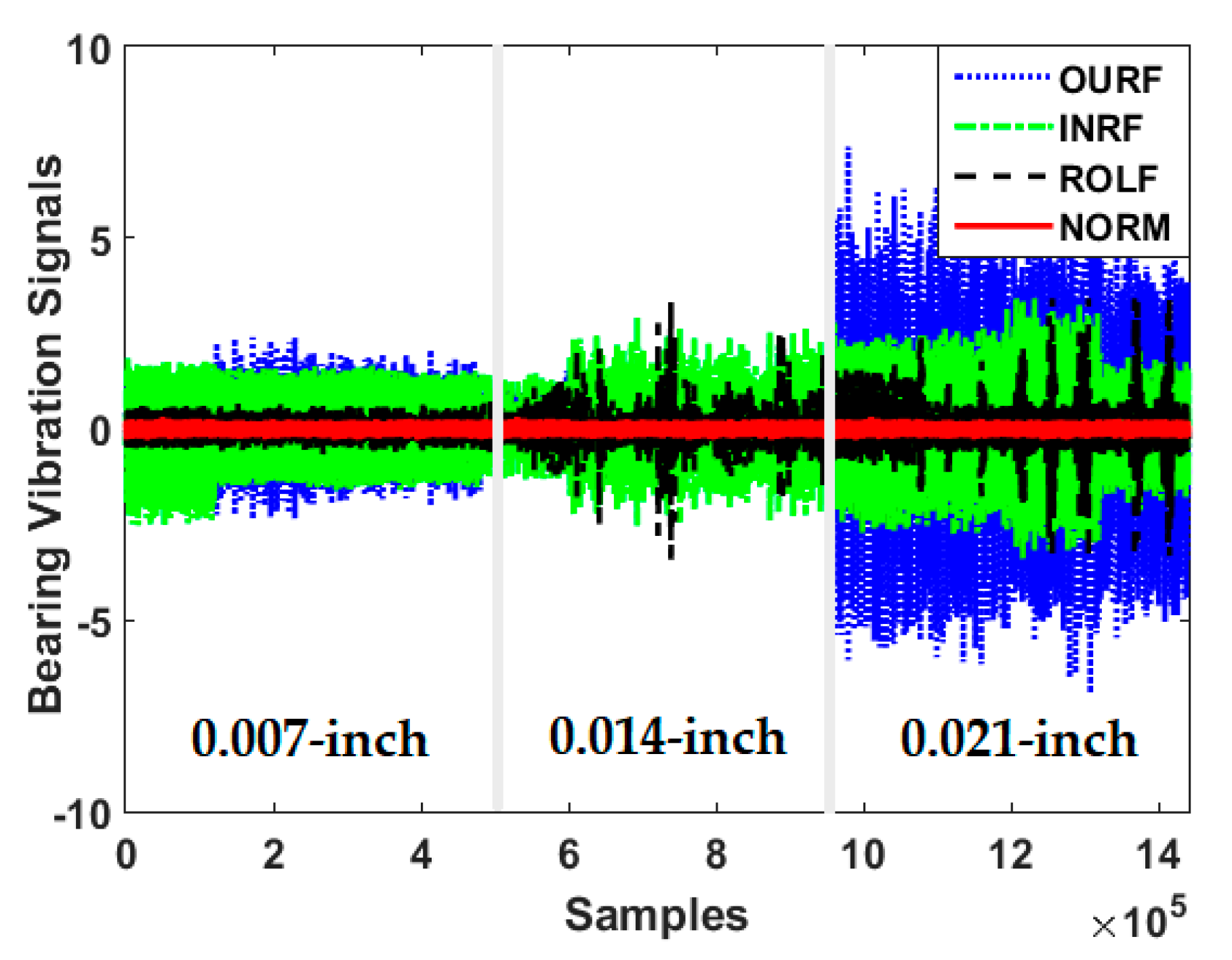
Figure 2 illustrates the original vibration signals in bearings under all conditions. As seen in the figure, when crack sizes are 0.007, 0.014, and 0.021 inches, the ROLF, INRF, and OURF overlap, causing misclassifications in fault diagnosis. Based on Figure 2, it can be seen that the classification of the original raw signals is very difficult because these signals are overlapped in abnormal conditions. To address this issue, the proposed algorithm is recommended.

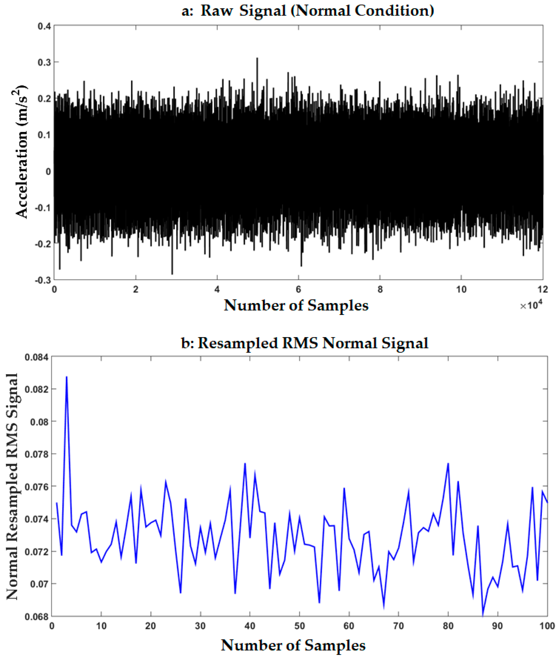
The normal Raw signal of bearing and the resampled RMS signal for the normal condition is illustrated in Figure 3.

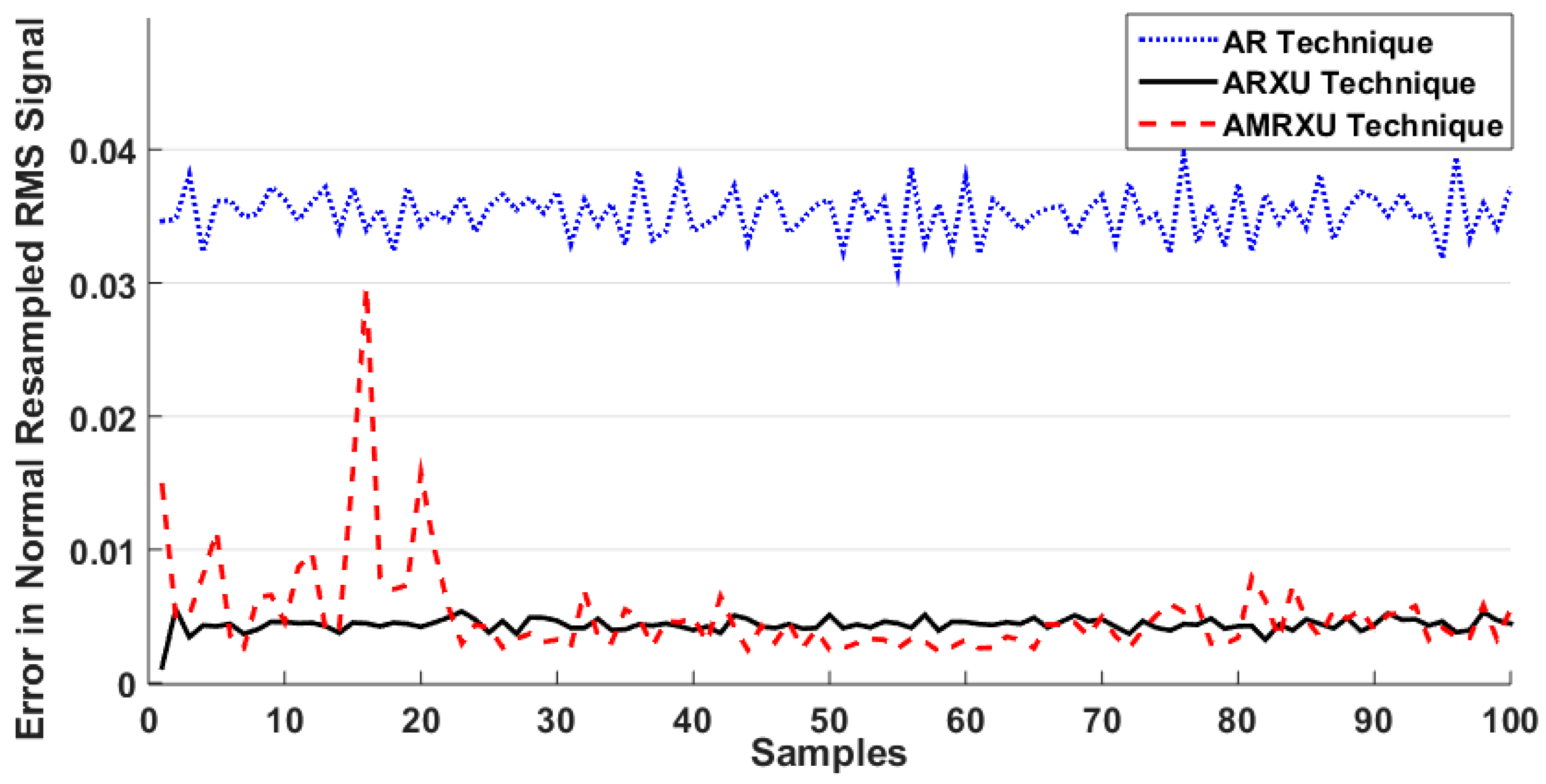
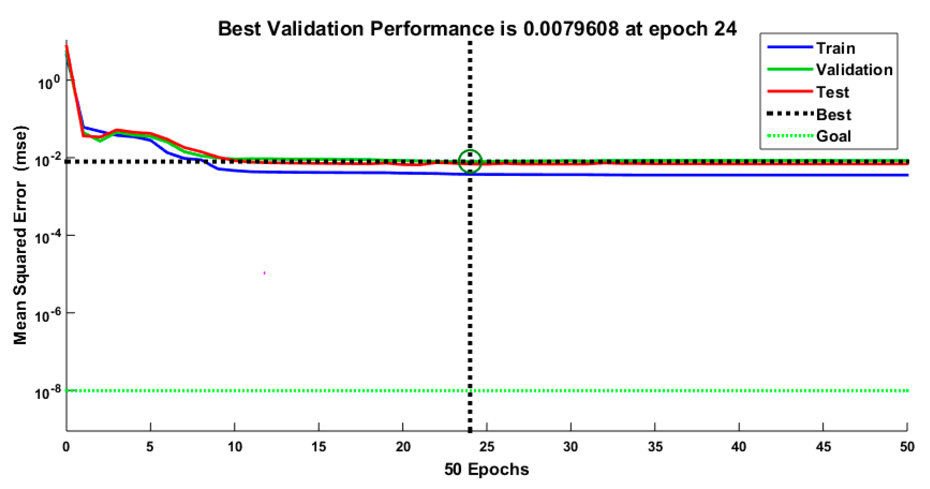
Figure 4 shows the error in signal modeling using the AR technique, the ARXU method, and the proposed AMRXU algorithm for resampled RMS signals in a normal state. In Figure 4, the accuracy of the normal resampled RMS signal modeled using AR is around 51.33%; by ARXU, it is around 85.5%, and based on AMRXU, the accuracy is 98.5%. Thus, the linear AR and ARXU approaches are not accurate enough to model the nonlinear and nonstationary signals. To address this issue, the nonlinear signal modeling approach using proposed AMRXU is suggested in this work. The mean square error (MSE) of the RMS resampled normal signal modeling using the AMRXU for training, validation, and testing is presented in Figure 5. From the figure, we can observe that MSE curves sharply decrease within the first 7 epochs until they reach the MSE level of near 0.01. Then, for the next 17 epochs, some oscillations can be approximated, and these curves converge to an MSE level of around 0.0079.

The AMRXU-PMI and AMRXU-VSPMI methods are inherently linear estimators and the most significant advantage for them is that we can perform model structure and parameter identification rapidly. The performance of signal pattern recognition in these techniques appears to be satisfactory. However, to increase the performance of fault diagnosis, pattern identification and crack size detection, the AMRXU-AVSPMI is suggested in the paper. 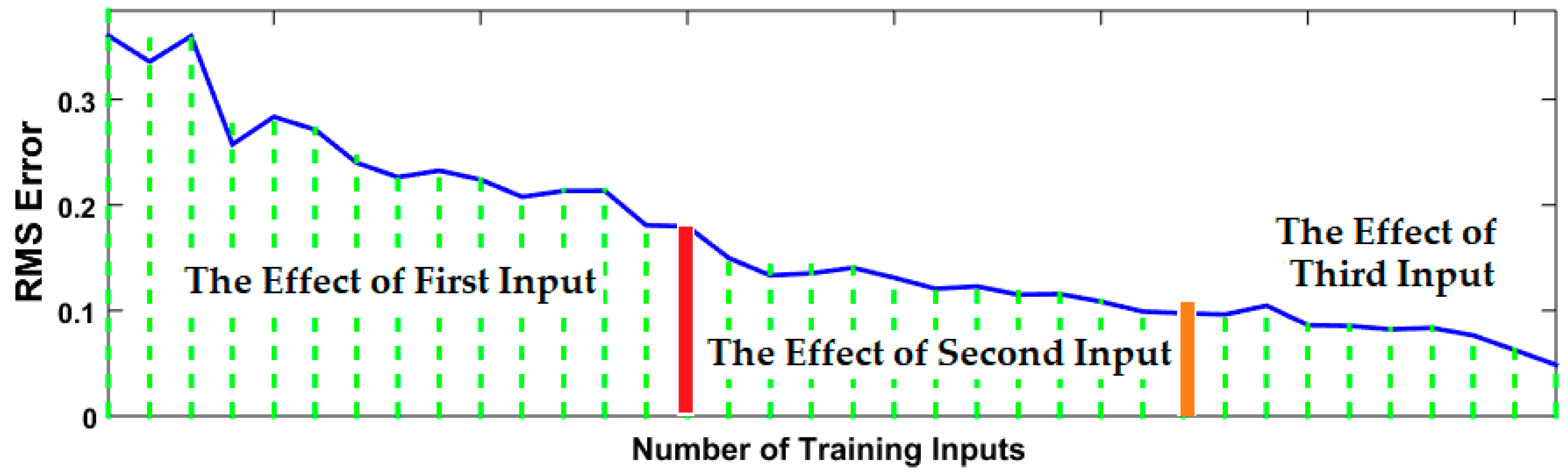Figure 6 shows the effect of the SNFS technique and training the inputs on the RMS error of signal estimation. In this case, the SNFS algorithm has 34 nodes, 32 linear parameters, 18 nonlinear parameters, and eight fuzzy rules. The elapsed time in this SNFS design is 0.223 s. To have the minimum RMS error, the first, second, and third inputs need to have 15-, 12-, and 9-times training, respectively.

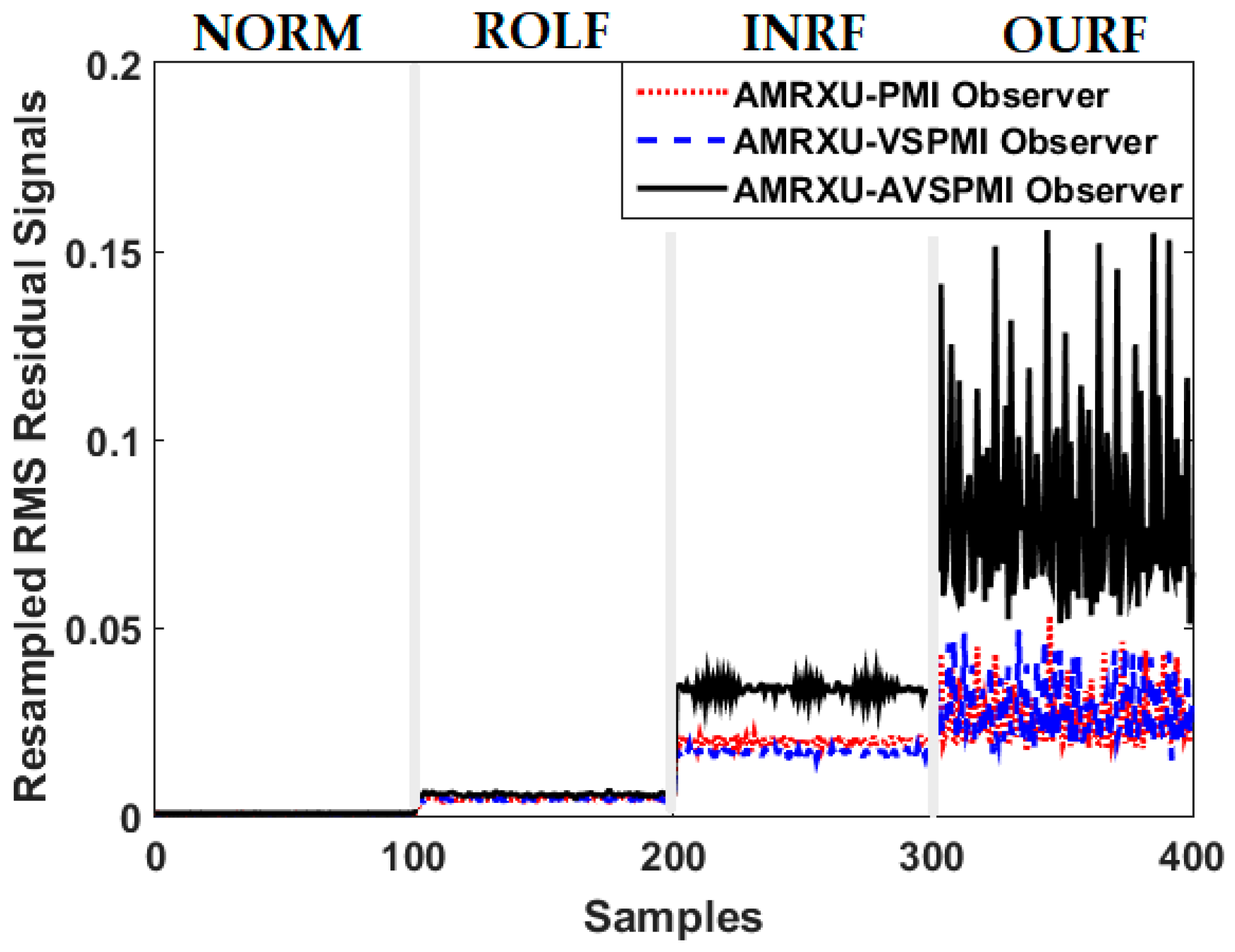
Figure 7 shows the power of estimation algorithms for signal classification using the proposed scheme (AMRXU-AVSPMI), the AMRXU-VSPMI technique, and the AMRXU-PMI method.

As seen in Figure 7, with the proposed AMRXU-AVSPMI technique, which is an adaptive hybrid-nonlinear observer, the RMS signal amplitude for the four classes is detectable. In the AMRXU-PMI method, which is a linear observer, the distinction between the inner and outer faults is either very low or indistinguishable. These conditions improved somewhat with the AMRXU-VSPMI technique, which is a robust observer, but were less detectable than with the proposed AMRXU-AVSPMI observer.

To test the accuracy of each state’s identification, a combination of the proposed scheme (AMRXU-AVSPMI) with an SVM (AMRXU-AVSPMI+SVM) is compared against AMRXU-VSPMI+SVM and AMRXU-PMI+SVM. The fault identification and classification performance for the methods mentioned above are assessed by using important metrics [46], such as averaged recall ($Re{c}_{av}$), averaged precision ($Pre{c}_{av}$), averaged F1-score ($F{1}_{av}$), and total fault identification and classification accuracy (FICA). We also use these metrics to test the robustness of the proposed methods. These metrics are defined as the following equations:

$$Re{c}_{av}=\frac{{{\displaystyle \sum }}_{k=1}^{K}T{P}_k}{{{\displaystyle \sum }}_{k=1}^K\left(T{P}_k+F{N}_k\right)}\times 100;$$

(46)

$$Pre{c}_{av}=\frac{{{\displaystyle \sum }}_{k=1}^{K}T{P}_k}{{{\displaystyle \sum }}_{k=1}^K\left(T{P}_k+F{P}_k\right)}\times 100;$$

(47)

$$F{1}_{av}=2\times \left(Pre{c}_{av}\times Re{c}_{av}\right)\times 100/\left(Pre{c}_{av}+Re{c}_{av}\right);$$

(48)

$$FICA=\frac{{{\displaystyle \sum }}_k^{K}TP{V}_k}{N}\times 100.$$

(49)

where, $T{P}_k$,$F{P}_k,F{N}_k$, $N$ are the true-positive value for the class of k, false-positive value for the class of k, and false-negative value for the class of $k$, and the data samples, respectively. Also, K is the number of classes, and k is the index of class such that k = 1, …, K. To test the robustness of the above algorithms, the results are tested in 10 experiments and summarized in

Table 4. The $Re{c}_{av}$, $Pre{c}_{av}$, $F{1}_{av}$, and FICA averaged over 10 experiments.

Methods	Metrics
	$\mathit{R}\mathit{e}{\mathit{c}}_{\mathit{a}\mathit{v}} (\%)$	$\mathit{P}\mathit{r}\mathit{e}{\mathit{c}}_{\mathit{a}\mathit{v}} (\%)$	$\mathit{F}{1}_{\mathit{a}\mathit{v}} (\%)$	FICA (%)
AMRXU-AVSPMI+SVM	97.9	97.84	97.84	97.8
AMRXU-VSPMI+SVM	95	94.83	94.84	94.8
AMRXU-PMI+SVM	90.9	90.9	90.9	90.85

.

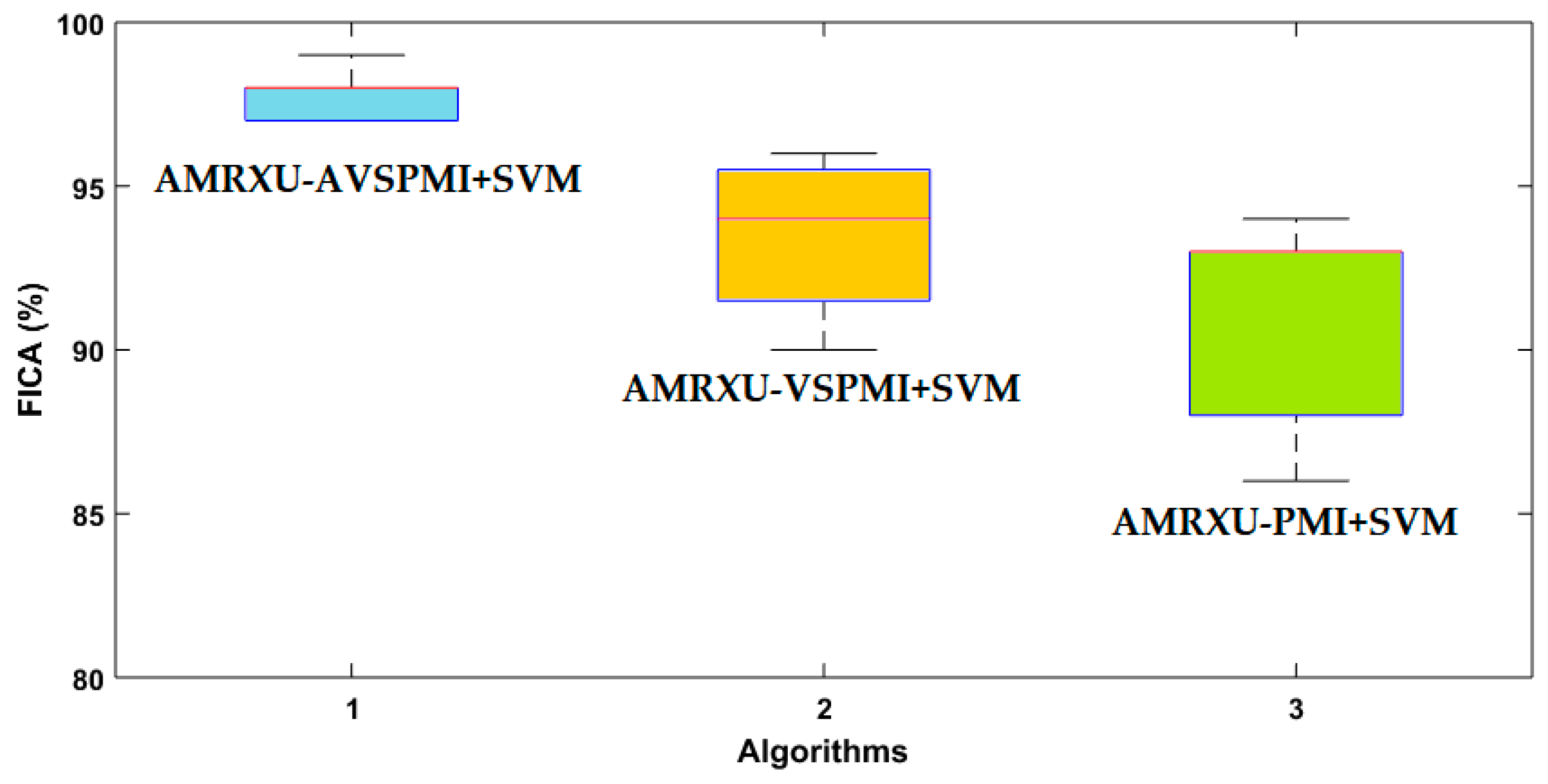
Figure 8 shows the boxplots of the FICA metric over 10 experiments for AMRXU-AVSPMI+SVM, AMRXU-VSPMI+SVM, and AMRXU-PMI+SVM. From Figure 8, it is observed that the classification accuracy of the proposed method (AMRXU-AVSPMI+SVM) is the most robust because it does not deviate meaningfully from the average of FICA, which validates the repeatability of the test. For AMRXU-VSPMI+SVM, the deviation of FICA is not very high; however, the average accuracy is lower than that of the proposed method. Unlike the proposed method, the AMRXU-PMI+SVM boxplot has a significant deviation from the average of the FICA. From Figure 8, we know that the combination of the AVSPMI observation technique, the modeling algorithm using AMRXU, and the SVM classifier can improve the classification and identification performance and fault diagnosis stability and robustness. 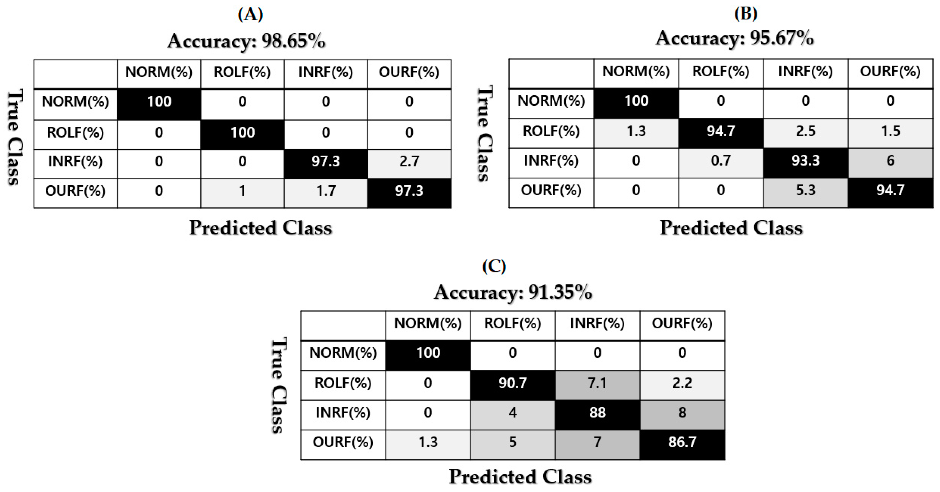Figure 9, Figure 10, Figure 11 and Figure 12 show the average of confusion matrices for 10 experiments to observe the specific details about the fault diagnosis performance when the torque load varies from 0 hp to 3 hp.

Table 5. The accuracy in state identification (torque load: 0 hp).

Technique	AMRXU-AVSPMI+SVM			AMRXU-VSPMI+SVM			AMRXU-PMI+SVM
Crack Sizes (in.)	0.007	0.014	0.021	0.007	0.014	0.021	0.007	0.014	0.021
NORM (%)	100	100	100	100	100	100	100	100	100
ROLF (%)	100	100	100	96	92	96	96	92	84
INRF (%)	96	100	96	92	92	96	92	88	84
OURF (%)	96	96	100	96	96	92	80	88	92
Average (%)	98	99	99	96	95	96	92	92	90

and Figure 9 demonstrate the accuracy of state identification when the torque load is 0 hp based on the proposed scheme (AMRXU-AVSPMI+SVM), AMRXU-VSPMI+SVM, and AMRXU-PMI+SVM.

From Figure 9, it is clear that AMRXU-VSPMI+SVM and AMRXU-PMI+SVM have high misclassification problems, especially between the inner and outer faults. The proposed AMRXU-AVSPMI+SVM reduced this challenge. Moreover, the average accuracy of state identification when the torque load was 0 hp from the proposed AMRXU-AVSPMI+SVM, AMRXU-VSPMI+SVM, and AMRXU-PMI+SVM was 98.65%, 95.67%, and 91.35%, respectively. Thus, the proposed AMRXU-AVSPMI+SVM improved the average state identification accuracy compared to AMRXU-VSPMI+SVM and AMRXU-PMI+SVM by around 2.98% and 7.3%, respectively.

Table 6. The accuracy in state identification (torque load: 1 hp).

Technique	AMRXU-AVSPMI+SVM			AMRXU-VSPMI+SVM			AMRXU-PMI+SVM
Crack Sizes (in.)	0.007	0.014	0.021	0.007	0.014	0.021	0.007	0.014	0.021
NORM (%)	100	100	100	100	100	100	100	100	100
ROLF (%)	96	100	100	92	92	96	88	92	88
INRF (%)	92	96	96	92	92	92	92	84	88
OURF (%)	100	96	96	96	92	92	80	88	92
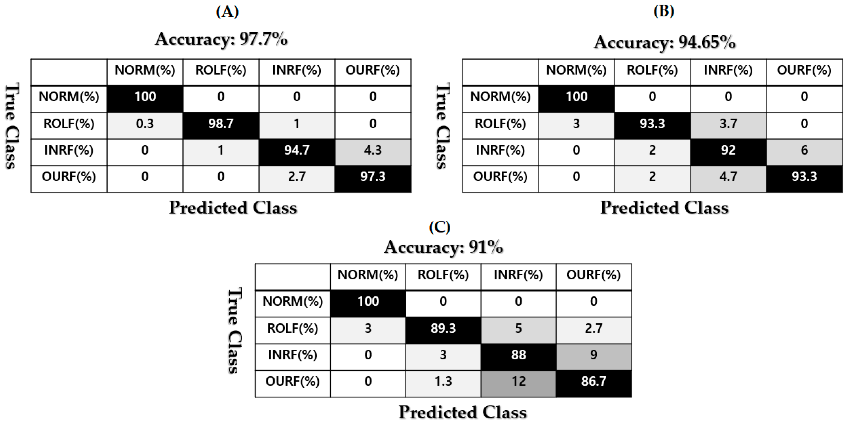
Average (%)	97	98	98	95	94	95	90	91	92

and Figure 10 demonstrate the accuracy in state identification when the torque load was 1 hp based on the proposed scheme (AMRXU-AVSPMI+SVM), on AMRXU-VSPMI+SVM, and on AMRXU-PMI+SVM.

Based on Figure 10 and Table 6, it is clear that AMRXU-PMI+SVM had a misclassification problem, especially between inner and outer faults, which the proposed AMRXU-AVSPMI+SVM method reduced. Furthermore, the average accuracy in state identification when the torque load was 1 hp with the proposed AMRXU-AVSPMI+SVM, with AMRXU-VSPMI+SVM, and with AMRXU-PMI+SVM was 97.7%, 94.65%, and 91%, respectively. Thus, the proposed AMRXU-AVSPMI+SVM improved average state identification accuracy compared to AMRXU-VSPMI+SVM and AMRXU-PMI+SVM by around 3.05% and 6.7%, respectively.

Table 7. The accuracy of state identification (torque load: 2 hp).

Technique	AMRXU-AVSPMI+SVM			AMRXU-VSPMI+SVM			AMRXU-PMI+SVM
Crack Sizes (in.)	0.007	0.014	0.021	0.007	0.014	0.021	0.007	0.014	0.021
NORM (%)	100	100	100	100	100	100	100	100	100
ROLF (%)	100	100	100	92	96	96	92	92	92
INRF (%)	92	96	96	92	92	96	88	88	84
OURF (%)	96	92	96	92	92	92	84	88	88
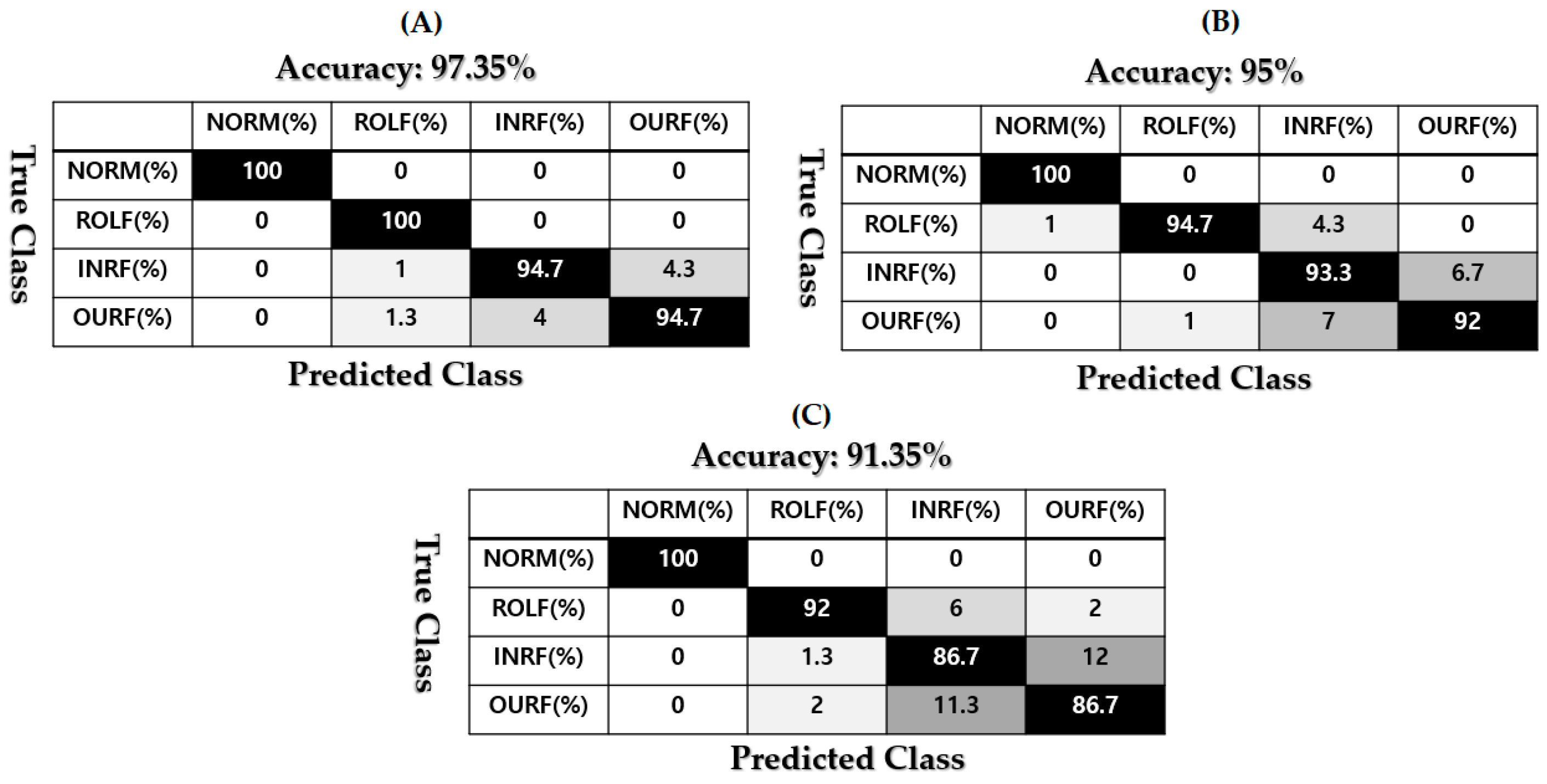
Average (%)	97	97	98	94	95	96	91	92	91

and Figure 11 demonstrate the accuracy in state identification when the torque load was 2 hp based on the proposed scheme (AMRXU-AVSPMI+SVM), on AMRXU-VSPMI+SVM, and on AMRXU-PMI+SVM.

In Table 7 and Figure 11, we can see that AMRXU-PMI+SVM and AMRXU-VSPMI+SVM had misclassification and overlap problems with inner and outer faults, but the proposed AMRXU-AVSPMI+SVM method reduced overlapping. Besides, the average accuracy in the state identification when the torque load was 2 hp in the proposed AMRXU-AVSPMI+SVM, AMRXU-VSPMI+SVM, and AMRXU-PMI+SVM was 97.35%, 95%, and 91.35%, respectively. Thus, the proposed AMRXU-AVSPMI+SVM improved average state identification accuracy from AMRXU-VSPMI+SVM and AMRXU-PMI+SVM by around 2.35% and 6%, respectively. Finally,

Table 8. The accuracy of state identification (torque load: 3 hp).

Technique	AMRXU-AVSPMI+SVM			AMRXU-VSPMI+SVM			AMRXU-PMI+SVM
Crack Sizes (in.)	0.007	0.014	0.021	0.007	0.014	0.021	0.007	0.014	0.021
NORM (%)	100	100	100	100	100	100	100	100	100
ROLF (%)	100	96	100	92	96	96	92	88	92
INRF (%)	96	96	96	92	92	88	84	88	80
OURF (%)	96	96	96	92	88	92	84	88	84
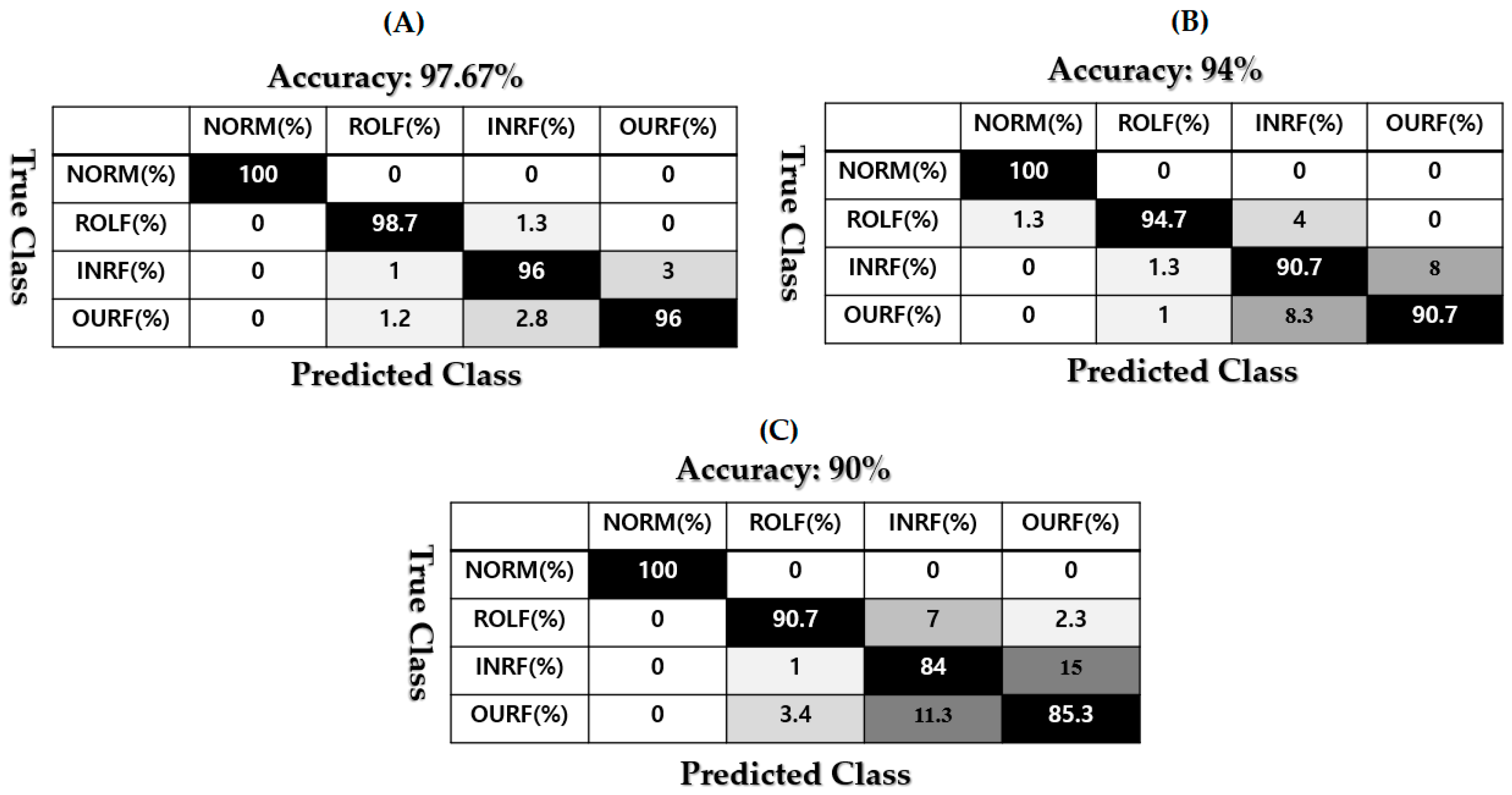
Average (%)	98	97	98	94	94	94	90	91	89

and Figure 12 show the accuracy in state identification when the torque load was 3 hp based on the proposed scheme (AMRXU-AVSPMI+SVM), on AMRXU-VSPMI+SVM, and on AMRXU-PMI+SVM.

The average fault pattern identification by the proposed AMRXU-AVSPMI+SVM, by AMRXU-VSPMI+SVM, and by AMRXU-PMI+SVM is demonstrated in

Table 9. The average accuracy in fault pattern identification from the proposed AMRXU-AVSPMI+SVM compared to AMRXU-VSPMI+SVM and AMRXU-PMI+SVM.

Method/Fault	NORM	ROLF	INRF	OURF
AMRXU-AVSPMI+SVM	100%	99.34%	95.67%	96.33%
AMRXU-VSPMI+SVM	100%	94.34%	92.33%	92.67%
AMRXU-PMI+SVM	100%	90.67%	86.67%	86.34%

. In Table 9, the accuracy in fault pattern detection from the proposed scheme, compared with AMRXU-VSPMI+SVM, increased for ROLF, INRF, and OURF defects by 5%, 3.34%, and 3.66%, respectively. Moreover, the accuracy in fault pattern detection from the proposed scheme, compared with AMRXU-PMI+SVM, for ROLF, INRF, and OURF defects improved by 8.67%, 9%, and 9.99%, respectively. Moreover, the average crack size detection in ROLF, INRF, and OURF from using AMRXU-AVSPMI+SVM, AMRXU-VSPMI+SVM, and AMRXU-PMI+SVM is shown in

Table 10. The average accuracy in roller crack size detection using the proposed AMRXU-AVSPMI+SVM compared to AMRXU-VSPMI+SVM, and AMRXU-PMI+SVM.

Method/Crack Size	0.007 in.	0.014 in.	0.021 in.	Average
AMRXU-AVSPMI+SVM	99%	99%	100%	99.33%
AMRXU-VSPMI+SVM	93%	94%	96%	94.33%
AMRXU-PMI+SVM	92%	91%	89%	90.67%

,

Table 11. The average accuracy for inner crack size detection using the proposed AMRXU-AVSPMI+SVM compared to AMRXU-VSPMI+SVM and AMRXU-PMI+SVM.

Method/Crack Size	0.007 in.	0.014 in.	0.021 in.	Average
AMRXU-AVSPMI+SVM	94%	97%	96%	95.67%
AMRXU-VSPMI+SVM	92%	92%	93%	92.33%
AMRXU-PMI+SVM	89%	87%	84%	86.67%

and

Table 12. The average accuracy for outer crack size detection from the proposed AMRXU-AVSPMI+SVM compared to AMRXU-VSPMI+SVM and AMRXU-PMI+SVM.

Method/Crack Size	0.007 in.	0.014 in.	0.021 in.	Average
AMRXU-AVSPMI+SVM	97%	95%	97%	96.33%
AMRXU-VSPMI+SVM	94%	92%	92%	92.67%
AMRXU-PMI+SVM	82%	88%	89%	86.33%

, respectively.

Table 10 shows the average accuracy in roller crack size detection using AMRXU-AVSPMI+SVM, AMRXU-VSPMI+SVM, and AMRXU-PMI+SVM. In this table, accuracy in roller crack size detection based on AMRXU-AVSPMI+SVM, AMRXU-VSPMI+SVM, and AMRXU-PMI+SVM was 99.33%, 94.33%, and 90.67%. In addition, the average accuracy in inner crack size detection using AMRXU-AVSPMI+SVM, AMRXU-VSPMI+SVM, and AMRXU-PMI+SVM is illustrated in Table 11. In this table, accuracy in inner crack size detection based on the AMRXU-AVSPMI+SVM improved (compared with AMRXU-VSPMI+SVM and AMRXU-PMI+SVM) by 3.34% and 9%, respectively. Moreover, the average accuracy from outer crack size detection using AMRXU-AVSPMI+SVM, AMRXU-VSPMI+SVM, and AMRXU-PMI+SVM is illustrated in Table 12. In this table, accuracy from outer crack size detection with AMRXU-AVSPMI+SVM improved in comparison with AMRXU-VSPMI+SVM and AMRXU-PMI+SVM by 3.66% and 10%, respectively.

The main reason that the accuracy of the fault diagnosis in the AMRXU-VSPMI and AMRXU-PMI algorithms is less than that of the proposed AMRXU-AVSPMI is due to the nature of the linear observation (AMRXU-VSPMI and AMRXU-PMI) algorithms. When these procedures are applied to the nonlinear and non-stationary such as bearing signals, the estimation error is developed compared to the nonlinear AMRXU-AVSPMI observation method. However, according to the concept of robustness, the performance of AMRXU-VSPMI is better than the AMRXU-PMI. Subsequently, the proposed hybrid framework is suitable for accurate fault diagnosis of the bearing in different crack sizes and torque loads in comparison with the other referenced methods. From the experimental results, it is obvious that the combination of the AVSPMI observation technique with the AMRXU modelling approach can improve the performance of the fault diagnosis in comparison with the linear observation technique. However, from Table 9, Table 10, Table 11 and Table 12, we can see that the inner and outer performance for fault pattern identification and crack size detection should be improved. Moreover, the preprocessing unit in the presence of the noisy signal must be improved by using filter techniques.

8. Conclusions

In the paper, a methodology has been developed to improve the fault diagnosis of a bearing by utilizing a hybrid observation. This methodology has been applied to a real case of an experimental CWRU dataset. Furthermore, within this method, the hybrid-based signal modeling for the normal resampled RMS signal using a smart autoregressive modeling approach with 98.5% accuracy was suggested. Moreover, to generate robust and reliable residual signals, the adaptive variable structure-Lyapunov proportional multi-integral observer was adopted. The support vector machine was recommended for the classification of residual signals. According to the experimental results, the average accuracy for crack size identification was 98.65%, 97.7%, 97.35%, and 97.67%, respectively, when the motor torque loads were 0 hp, 1 hp, 2 hp, and 3 hp. In addition, the average pattern identification for NORM, ROLF, INRF, and OURF was 100%, 99.34%, 95.67%, and 96.33%, respectively. The results suggest that the proposed approach was useful for the diagnosis of bearing failures. On the other hand, this approach could also be recommended in other systems such as condition monitoring. In that case, it would be important to consider some important factors such as the sampling rate frequency and motor rotational speeds to adapt the preprocessing stage since the accuracy of the fault diagnosis depends on them. In future work, we will focus on the improvement of the robustness, reliability, and precision of the proposed scheme. One of the possible directions for the improvement is to discover the robust function approximation by using a combination of the mathematical-based technique and data-driven-based signal modeling approach. Another direction is to improve the estimation algorithm by using the nonlinear architecture of the observation approach where we can combine the nonlinear robust observer with a deep learning approach to increase the performance of signal estimation and classification and reduce the complexity. Furthermore, the problem of different conditions/datasets should be analyzed, and the proposed algorithm needs to be validated by using the vibration and acoustic emission datasets with various motor speeds, torque loads, and crack sizes.

References

1. Yu, X.; Dong, F.; Ding, E.; Wu, S.; Fan, C. Rolling Bearing Fault Diagnosis Using Modified LFDA and EMD With Sensitive Feature Selection. IEEE Access 2018, 6, 3715–3730. [Google Scholar] [CrossRef]
2. Jiang, W.; Hong, Y.; Zhou, B.; He, X.; Cheng, C. A GAN-based anomaly detection approach for imbalanced industrial time series. IEEE Access 2019, 7, 143608–143619. [Google Scholar] [CrossRef]
3. Garcia-Perez, A.; de Jesus Romero-Troncoso, R.; Cabal-Yepez, E.; Osornio-Rios, R.A. The application of high-resolution spectral analysis for identifying multiple combined faults in induction motors. IEEE Trans. Ind. Electron. 2011, 58, 2002–2010. [Google Scholar] [CrossRef]
4. Lei, Y.; Li, N.; Guo, L.; Li, N.; Yan, T.; Lin, J. Machinery health prognostics: A systematic review from data acquisition to RUL prediction. Mech. Syst. Signal Process. 2018, 104, 799–834. [Google Scholar] [CrossRef]
5. Lei, Y. Introduction and Background. In Intelligent Fault Diagnosis and Remaining Useful Life Prediction of Rotating Machinery; Xi’an Jiaotong University Press: Xi’an, China, 2016; pp. 1–16. [Google Scholar]
6. Calabrese, F.; Regattieri, A.; Botti, L.; Mora, C.; Galizia, F.G. Unsupervised Fault Detection and Prediction of Remaining Useful Life for Online Prognostic Health Management of Mechanical Systems. Appl. Sci. 2020, 10, 4120. [Google Scholar] [CrossRef]
7. Calabrese, F.; Regattieri, A.; Botti, L.; Galizia, F.G. Prognostic Health Management of Production Systems. New Proposed Approach and Experimental Evidences. Procedia Manuf. 2019, 39, 260–269. [Google Scholar] [CrossRef]
8. Mao, W.; Feng, W.; Liang, X. A novel deep output kernel learning method for bearing fault structural diagnosis. Mech. Syst. Signal Process. 2019, 117, 293–318. [Google Scholar] [CrossRef]
9. Chegini, S.N.; Manjili, M.J.H.; Bagheri, A. New fault diagnosis approaches for detecting the bearing slight degradation. Meccanica 2020, 55, 261–286. [Google Scholar] [CrossRef]
10. Liu, Z.; Zhang, L. A review of failure modes, condition monitoring and fault diagnosis methods for large-scale wind turbine bearings. Measurement 2020, 149, 107002. [Google Scholar] [CrossRef]
11. Lee, J.; Wu, F.; Zhao, W.; Ghaffari, M.; Liao, L.; Siegel, D. Prognostics and health management design for rotary machinery systems—Reviews, methodology and applications. Mech. Syst. Signal Process. 2014, 42, 314–334. [Google Scholar] [CrossRef]
12. Carino, J.A.; Delgado-Prieto, M.; Iglesias, J.A.; Sanchis, A.; Zurita, D.; Millan, M.; Redondo, J.A.O.; Romero-Troncoso, R. Fault Detection and Identification Methodology Under an Incremental Learning Framework Applied to Industrial Machinery. IEEE Access 2018, 6, 49755–49766. [Google Scholar] [CrossRef]
13. Shin, I.; Lee, J.; Lee, J.Y.; Jung, K.; Kwon, D.; Youn, B.D.; Jang, H.S.; Choi, J.-H. A Framework for Prognostics and Health Management Applications toward Smart Manufacturing Systems. Int. J. Precis. Eng. Manuf. Technol. 2018, 5, 535–554. [Google Scholar] [CrossRef]
14. Zhang, P.; Lu, D. A survey of condition monitoring and fault diagnosis toward integrated O&M for wind turbines. Energies 2019, 12, 2801. [Google Scholar]
15. Boudiaf, A.; Moussaoui, A.; Dahane, A.; Atoui, I. A Comparative Study of Various Methods of Bearing Faults Diagnosis Using the Case Western Reserve University Data. J. Fail. Anal. Prev. 2016, 16, 271–284. [Google Scholar] [CrossRef]
16. Camci, F.; Medjaher, K.; Zerhouni, N.; Nectoux, P. Feature evaluation for effective bearing prognostics. Qual. Reliab. Eng. Int. 2013, 29, 477–486. [Google Scholar] [CrossRef] [Green Version]
17. Gupta, P.; Pradhan, M. Fault detection analysis in rolling element bearing: A review. Mater. Today Proc. 2017, 4, 2085–2094. [Google Scholar] [CrossRef]
18. Piltan, F.; Prosvirin, A.E.; Jeong, I.; Im, K.; Kim, J. Rolling-Element Bearing Fault Diagnosis Using Advanced Machine Learning-Based Observer. Appl. Sci. 2019, 9, 5404. [Google Scholar] [CrossRef] [Green Version]
19. Gao, Z.; Cecati, C.; Ding, S.X. A survey of fault diagnosis and fault-tolerant techniques—Part I: Fault diagnosis with model-based and signal-based approaches. IEEE Trans. Ind. Electron. 2015, 62, 3757–3767. [Google Scholar] [CrossRef] [Green Version]
20. Cecati, C. A survey of fault diagnosis and fault-tolerant techniques—Part II: Fault diagnosis with knowledge-based and hybrid/active approaches. IEEE Trans. Ind. Electron. 2015, 62, 3768–3774. [Google Scholar]
21. Sohaib, M.; Kim, C.; Kim, J. A hybrid feature model and deep-learning-based bearing fault diagnosis. Sensors 2017, 17, 2876. [Google Scholar] [CrossRef] [PubMed] [Green Version]
22. Ben Njima, C.; Garna, T. PIO Output Fault Diagnosis by ARX-Laguerre Model Applied to 2 nd Order Electrical System. IEEE Access 2020, 8, 83052–83061. [Google Scholar] [CrossRef]
23. Prosvirin, A.E.; Piltan, F.; Kim, J. Hybrid Rubbing Fault Identification Using a Deep Learning-Based Observation Technique. IEEE Trans. Neural Netw. Learn. Syst. 2020, 59, 10–24. [Google Scholar] [CrossRef] [PubMed]
24. Chen, K.; Huang, C.; He, J. Fault detection, classification and location for transmission lines and distribution systems: A review on the methods. High Volt. 2016, 1, 25–33. [Google Scholar] [CrossRef]
25. Yuan, H.; Dai, H.; Wei, X.; Ming, P. Model-based observers for internal states estimation and control of proton exchange membrane fuel cell system: A review. J. Power Sources 2020, 468, 228376. [Google Scholar] [CrossRef]
26. Zhuge, Q.; Lu, Y.; Yang, S. Non-stationary modelling of vibration signals for monitoring the condition of machinery. Mech. Syst. Signal Process. 1990, 4, 355–365. [Google Scholar] [CrossRef]
27. Sun, R.-B.; Yang, Z.-B.; Gryllias, K.; Chen, X.-F. Cyclostationary modeling for local fault diagnosis of planetary gear vibration signals. J. Sound Vib. 2020, 471, 115175. [Google Scholar] [CrossRef]
28. Chaari, F.; Zimroz, R.; Bartelmus, W.; Fakhfakh, T.; Haddar, M. Model based investigation on a two stages gearbox dynamics under non-stationary operations. In Condition Monitoring of Machinery in Non-Stationary Operations; Springer: Berlin/Heidelberg, Germany, 2012; pp. 133–142. [Google Scholar]
29. Mishra, C.; Samantaray, A.; Chakraborty, G. Ball bearing defect models: A study of simulated and experimental fault signatures. J. Sound Vib. 2017, 400, 86–112. [Google Scholar] [CrossRef]
30. Najeh, T.; Mbarek, A.; Bouzrara, K.; Nabli, L.; Messaoud, H. New methods of Laguerre pole optimization for the ARX model expansion on Laguerre bases. ISA Trans. 2017, 70, 93–103. [Google Scholar] [CrossRef] [PubMed]
31. Østergård, T.; Jensen, R.L.; Maagaard, S.E. A comparison of six metamodeling techniques applied to building performance simulations. Appl. Energy 2018, 211, 89–103. [Google Scholar] [CrossRef]
32. Singh, K.B.; Arat, M.A.; Taheri, S. Literature review and fundamental approaches for vehicle and tire state estimation. Veh. Syst. Dyn. 2019, 57, 1643–1665. [Google Scholar] [CrossRef]
33. Piltan, F.; Kim, J.-M. Bearing Fault Diagnosis Using an Extended Variable Structure Feedback Linearization Observer. Sensors 2018, 18, 4359. [Google Scholar] [CrossRef] [Green Version]
34. Tayebi Haghighi, S.; Koo, I. Fault Diagnosis of Rotating Machine Using an Indirect Observer and Machine Learning. In Proceedings of the 2020 International Conference on Information and Communication Technology Convergence (ICTC), Jeju Islan, Korea, 21–23 October 2020; pp. 277–282. [Google Scholar]
35. Senanayaka, J.S.L.; van Khang, H.; Robbersmyr, K.G. Towards online bearing fault detection using envelope analysis of vibration signal and decision tree classification algorithm. In Proceedings of the 2017 20th International Conference on Electrical Machines and Systems (ICEMS), Sydney, Australia, 11–14 August 2017; pp. 1–6. [Google Scholar]
36. Sharma, A.; Jigyasu, R.; Mathew, L.; Chatterji, S. Bearing Fault Diagnosis Using Weighted K-Nearest Neighbor. In Proceedings of the 2018 2nd International Conference on Trends in Electronics and Informatics (ICOEI), Tirunelveli, India, 11–12 May 2018; pp. 1132–1137. [Google Scholar]
37. Zhou, S.; Qian, S.; Chang, W.; Xiao, Y.; Cheng, Y. A novel bearing multi-fault diagnosis approach based on weighted permutation entropy and an improved SVM ensemble classifier. Sensors 2018, 18, 1934. [Google Scholar] [CrossRef] [Green Version]
38. Case Western Reserve University. Seeded Fault Test Data. Available online: http://csegroups.case.edu/bearingdatacenter/home (accessed on 22 March 2017).
39. Hadid, B.; Duviella, E.; Lecoeuche, S. Data-driven modeling for river flood forecasting based on a piecewise linear ARX system identification. J. Process. Control 2020, 86, 44–56. [Google Scholar] [CrossRef]
40. Galrinho, M.; Everitt, N.; Hjalmarsson, H. ARX modeling of unstable linear systems. Automatica 2017, 75, 167–171. [Google Scholar] [CrossRef] [Green Version]
41. Lei, Z.; Su, W. Mold Level Predict of Continuous Casting Using Hybrid EMD-SVR-GA Algorithm. Processes 2019, 7, 177. [Google Scholar] [CrossRef] [Green Version]
42. Parveen, N.; Zaidi, S.; Danish, M. Support vector regression (SVR)-based adsorption model for Ni (II) ions removal. Groundw. Sustain. Dev. 2019, 9, 100232. [Google Scholar] [CrossRef]
43. Karaboga, D.; Kaya, E. Adaptive network based fuzzy inference system (ANFIS) training approaches: A comprehensive survey. Artif. Intell. Rev. 2019, 52, 2263–2293. [Google Scholar] [CrossRef]
44. Sun, A.; Lim, E.-P.; Liu, Y. On strategies for imbalanced text classification using SVM: A comparative study. Decis. Support Syst. 2009, 48, 191–201. [Google Scholar] [CrossRef]
45. Konar, P.; Chattopadhyay, P. Bearing fault detection of induction motor using wavelet and Support Vector Machines (SVMs). Appl. Soft Comput. 2011, 11, 4203–4211. [Google Scholar] [CrossRef]
46. Sokolova, M.; Lapalme, G. A systematic analysis of performance measures for classification tasks. Inf. Process. Manag. 2009, 45, 427–437. [Google Scholar] [CrossRef]
Figure 1. The proposed scheme for fault diagnosis of bearing based on three stages: preprocessing, signal approximation and estimation, and fault classification.
Applsci 11 02784 g001
Figure 2. Bearing vibration signals for normal bearings and for ball, inner, and outer faults.
Applsci 11 02784 g002
Figure 3. RAW signals and resample signals: (a) the normal raw signal of a bearing, and (b) the resampled RMS signal extracted from the raw signal.
Applsci 11 02784 g003
Figure 4. Error in AR, ARXU, and AMRXU techniques from normal resampled RMS signal modeling.
Applsci 11 02784 g004
Figure 5. Training, validation, and testing MSE curves during RMS resampled normal signal modeling using AMRXU.
Applsci 11 02784 g005
Figure 6. Effect of the SNFS on reducing the signal estimation error.
Applsci 11 02784 g006
Figure 7. Resampled RMS residual signals under normal and abnormal conditions using AMRXU-PMI, AMRXU-VSPMI, and the proposed AMRXU-AVSPMI observers.
Applsci 11 02784 g007
Figure 8. The boxplots of the FICA metric over 10 experiments for the AMRXU-AVSPMI+SVM, AMRXU-VSPMI+SVM, and AMRXU-PMI+SVM.
Applsci 11 02784 g008
Figure 9. The average fault identification accuracy based on (A) the proposed AMRXU-AVSPMI+SVM, (B) AMRXU-VSPMI+SVM, and (C) AMRXU-PMI+SVM (torque load: 0 hp).
Applsci 11 02784 g009
Figure 10. The average fault identification accuracy based on (A) the proposed AMRXU-AVSPMI+SVM, (B) AMRXU-VSPMI+SVM, and (C) AMRXU-PMI+SVM (torque load: 1 hp).
Applsci 11 02784 g010
Figure 11. The average fault identification accuracy based on (A) the proposed AMRXU-AVSPMI+SVM, (B) AMRXU-VSPMI+SVM, and (C) AMRXU-PMI+SVM (torque load: 2 hp).
Applsci 11 02784 g011
Figure 12. The average fault identification accuracy based on (A) the proposed AMRXU-AVSPMI+SVM, (B) AMRXU-VSPMI+SVM, and (C) AMRXU-PMI+SVM (torque load: 3 hp).
Applsci 11 02784 g012