Abstract
In recent years in mobile robotics, the focus has been on methods, in which the fusion of measurement data from various systems leads to models of the environment that are of a probabilistic type. The cognitive model of the environment is less accurate than the exact mathematical one, but it is unavoidable in the robot collaborative interaction with a human. The subject of the research proposed in this paper is the development of a model for learning and planning robot operations. The task of operations and mapping the unknown environment, similar to how humans do the same tasks in the same conditions has been explored. The learning process is based on a virtual dynamic model of a mobile robot, identical to a real mobile robot. The mobile robot’s motion with developed artificial neural networks and genetic algorithms is defined. The transfer method of obtained knowledge from simulated to a real system (Sim-To-Real; STR) is proposed. This method includes a training step, a simultaneous reasoning step, and an application step of trained and learned knowledge to control a real robot’s motion. Use of the basic cognitive elements language, a robot’s environment, and its correlation to that environment is described. Based on that description, a higher level of information about the mobile robot’s environment is obtained. The information is directly generated by the fusion of measurement data obtained from various systems.
1. Introduction
Intelligent robotics is a merged field intersection of two other engineering fields, artificial intelligence (AI) and robotics. Standard data-based learning methods provide useful results, but they are not nearly similar to human behavior. Developed approaches of Deep Reinforcement Learning (DRL) can be used to learn and train robots for achieving high performance in the moving tasks [1]. Neural networks and machine learning have been increasingly used tool in all parts of society. Thus, mobile robot behavior in simulations and virtual robot models of identical real robots will significantly impact the world’s future. Let us look at the solutions that have become common today, particularly simulations, and apply the obtained results to the real systems. This is perhaps most notable in the Computer Aided Design/Computer Aided Manufacturing/Computer Numerical Control (CAD/CAM/CNC) production chain [2]. Many authors deal with problems where robots solve work scenes that are complex, unpredictable, and unstructured. Liu et al. [3] described a method of training a virtual agent in a simulated environment with the aim of reaching a random target position from a random initial position. The virtual agent path sequence obtained by simulation training is converted into a real robot command with control coordinate transformation for the robot that performs tasks. It should be mentioned that many authors present outcomes of learning simulation without testing them on real robot systems. Implementing experimental results in two different robot control tasks on real root systems has been shown in [4], which is a rare example of a real robot system experiment. A convolutional neural network’s development to control a home surveillance robot has been described in [5].
In this study, the considered mobile robot of the differential structure is equipped with an SoC computer card to control motion and collect range sensor data about the environment. A camera is used as a distance data values input for the neural network, i.e., a sensor for collecting input distance values into the neural network. Wang et al. [6] also used a camera as input distance data. The primary use of a camera in [6] is to control the formation of robots based on vision data captured from it. The developed controller loop requires only image data from a calibrated perspective camera mounted in any position and orientation on the robot. A mobile robots’ motion path planning method based on a cloud of points has been presented in [7].
The low amount of data processing power and random-access memory in personal computers available to the average user should be pointed out. The camera as a sensor for collecting input distance data seems to be the most convenient in information enrichment. However, it demands large amounts of data to be collected, processed, and stored in real-time without data loss. Szegedy et al. [8] described the mentioned problems. The problem of defining the mobile robot’s environment and finding the path between two points has begun to be solved in the early 1980s. The dominant solving methods have been the configuration environment method, potential fields method, and the equidistant paths method.
Previously mentioned methods are strictly deterministic, and they are not nearly similar to the way a human does it. They are based on the total processing power of computer instead of being cognitive. Crneković et al. [9,10,11,12,13,14] described the mobile robot’s cognitive ability, which was used in this research with modifications in the dynamic structure. In the meantime, sensors with the ability to collect a large amount of information (cameras and range sensors) appeared on the market. The processing of this information has also become local (System on Chip; SoC computers, in this research, RaspberryPi), which significantly changed the approach to solving problems. The starting point was no longer the assumption that all objects in the environment are fixed and known, but it has changed to the idea of the simultaneous and gradual construction of an environment model called the Simultaneous Localization And Mapping (SLAM) problem.
The models constructed with data from laser range sensors were in the form of clouds of points, which again led to coordinate systems and a numerical form of data that is difficult for a human to accept if person is unfamiliar with the mathematical definition of environment. We have highly qualified staff (engineers) who can work with complex systems such as robots (engineers understand coordinate systems, kinematics, control, programing languages) in production processes. The use of robots in households must be adapted to unprofessional operators who do not have engineering training. It means that such a mobile robot should have built-in cognitive abilities to understand the environment in which it is placed (room, chair, man, moving forward, the advantage of passing, the feature of decency). It is an extensive task that many research teams and companies will be working on in the future, and it surely will be a priority in financial investments.
The solution to these problems remains a current challenging problem. The transfer method of gained knowledge from simulated to a real system (Sim-To-Real; STR) is proposed in this paper. This method includes a training step, a simultaneous reasoning step, and an application step of what is trained and learned to control the real robot’s motion. In the real simulation training step, the simulated environment relevant to the task is created based on semantic information from the real scene and a coordinate transformation. Then, learned data is trained by the STR method in the built simulated environment, using neural networks and genetic algorithms as control logic. In the simultaneous reasoning step, learned cognitive behavior is directly applied to a robot system in real-world scenes without any of predefined real-world data. Experimental results in several different robot control tasks show that the proposed STR method can train cognitive abilities with high generalized performance and significantly low training costs. In recent years, researchers have been using neural networks during learning and training robots’ behavior in various fields, expecting that the results obtained in the simulations will be applicable in real-world situations.
Collecting data about the environment in which a robot needs to move, in a cognitive way the way a human does, is costly, potentially unsafe, and time-consuming on real robot systems. Learning and training processes for real robots can be difficult and tedious. One promising strategy is to create virtual models of mobile robots in simulated environments in which data collection is safe and convenient in terms of reducing high costs. In simulated environments, it is also achievable to have a high success rate in transferring learned and trained knowledge to real-world systems. However, it is highly resource-consuming to create simulated environments similar to real-world scenes, especially with excellent fidelity. Consequently, procedures learned and trained in simulated environments usually cannot directly execute successfully in the real world due to the simulation-reality gap (discrepancies between the simulated and real environments) [4].
This research limits the possibility of a cognitive description of the closed (limited) environment where a mobile robot was placed. The limit has been given to achieve the possibility of a robot’s communication with a human. An example of communication is the human’s question “Where are my car keys?”, the usual answer would be “Car keys are at coordinates 578, 312, 105.”, while the robot’s with cognitive abilities answer would be “Car keys are on the dresser in the living room”. If the additional request to the robot is “Bring the keys”, we would expect it not to collide with a wall, a chair, another person, or not to get stuck on the edge of the table and crash the glass vase. So, we expect a smooth, elegant, human-like movement through the environment when executing a given task.
In recent studies, it is possible to find various approaches to solving these problems. Still, most systems use a camera as the primary sensor for determining the position of an object, which has to be intercepted, avoided, or bypassed [15,16]. The fusion of the obtained information from various sensors was used in the system presented in [17]. The authors have proposed solutions for locating, navigating, and planning the motion paths of different types of mobile robots placed in different environments [18]. More and more authors use virtual reality software tools for virtual modelling of identical systems to real systems [19,20,21]. One of the best software platforms for virtual simulations, entirely free for research purposes, is described in [22,23]. Many authors use it to simulate aircraft design and testing steps [24]. Others use it to simulate industrial, underwater and other robot mechanisms [25,26].
An increasing number of authors [21,27,28] use a virtual reality simulation platform to simulate the mobile robot’s autonomous behavior. A comparison and possibilities of software tools for simulating mobile robot model’s behavior, connected to environment sensors and integrated into the same, virtually defined environments, are given by Ivaldi et al. [29].
For the needs of the research presented in this paper, a virtual environment for the equipment partially described in papers [11,12,13] is developed. The mobile robot that has been partially described in the article [11] is also upgraded with higher-quality drive motors, laser range sensor and a newer generation control computer with better computational properties (Figure 1). Information data from the internal and external environment (laser range sensors) and motion (motor encoders) sensors are implemented and formatted to the appropriate form. All sensors are mounted on the mobile robot placed in real environment-polygon.
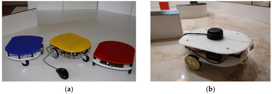
Figure 1.
Mobile robots: (a) an older generation equipped with Infrared (IR) range sensors; (b) a newer generation equipped with laser range sensors.
The achieved contributions of the research presented in this paper are as follows. The developed models and algorithms are stated, and possible application areas are described. A cognitive model of the closed environment of a mobile robot is constructed. The environment model is constructed with a fusion of various data, such as robot position and orientation data, monitoring information about objects seen by the camera above the robot, and information from laser range sensors and encoders attached to the robot motors. By fusing all this information, new information is obtained that is more than a simple sum of data parts. After the robot starts exploring an unknown enclosed environment, it moves through the entire environment within an adequate exploration time. At the end of exploration, robot reports that environment is now known, and with the help of basic cognitive elements, the robot provides environment elements position and basic description. Using the basic cognitive elements language, the robot’s environment and its correlation to that environment are described. Based on this description, a higher level of information about the robot’s environment is obtained, by fusion of earlier mentioned measurement data collected from various sensor devices. Recommendations and guidelines for continued future research are given.
The rest of paper is organized as follows. In Section 2, the primary goal of the research is established. Research work plan and research methodology are presented. Furthermore, the definition of tasks and terms are established. In Section 3, a definition of robot motion with mathematical models of the mobile robot system is described. The cognitive model of the closed environment (developed algorithms for a cognitive behavior of the mobile robot) is thoroughly described in Section 4. In Section 5, the development process of a mechatronic system used in research is described. In Section 6, experimental validation of the developed control model and the obtained results are described in detail. The results obtained on the developed real mobile robot system were compared with those obtained by simulations. The applicability of the developed algorithms on a real robot system has been confirmed. This outcome is described in Section 7. In Section 8, an evaluation of the obtained results is discussed, and a critical review is given.
2. Problem Description
2.1. Cognitive Robotics and Robot Path Planning
It is essential to explain how humans perceive their environment, both statically and dynamically, followed by the decision for some action. Instead of precise numerical values describing spatial metrics, the mental environment is established and described with identifying obstacles’ properties and their correlation to the environment. Specific agents are activated to find specific properties. Complex properties are constructed from simpler ones. It is assumed that if we have such a model and goal of the movement, it is possible to activate the start trigger of the particular motion. In this way, only one step of motion is determined with a plan for several steps forward. The desire to build a robot similar to a human, not only in appearance but also in behavior, has introduced new areas into robotics, unimaginable before. Fortunately, additional decision-making tools have been developed: fuzzy logic, artificial intelligence, artificial neural networks, genetic algorithms, visual recognition, voice analysis, parallel programing, agent systems. These tools have brought the cognitive realization that we have constructive elements for the systems with human-like behavior (robots), recognized by their cognitive abilities.
2.2. Cognitive Model of Mobile Robot’s Environment
This paper tries to answer the minimum set of topological designations and their sufficient properties for independent robot path planning from start to finish. The answer gives an environment model classified as a cognitive environment model because it resembles a human environment model. The cognitive environment model can be divided into parts called districts. At any time, the mobile robot can define what it sees from its current position. Although the cognitive model description is not as accurate as of the numerical approach, it can be designed in a much simpler way and is very effective, as human evolution proves. For the simulation, the environment in which the robot explores does not have to be known. Obstacles are defined as polygons by a set of points. The starting point of the robot’s motion path is always from an angle, that is also the centre of the coordinate system used for the simulation. It implicates that the initial position of the robot is known, as starting condition. Environment objects, such as obstacles, are placed in the environment configuration file. During the robot motion simulation, it is necessary to check the robot’s possibility of collision with other obstacles placed in the environment polygon. A virtual polygon is shown in Figure 2. Collision checks must be executed before every simulation step.
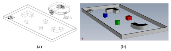
Figure 2.
Main elements used in research: (a) virtual polygon with a mobile robot (scale 1:1); (b) random scene of virtual polygon for robot exploration, used for real polygon environment construction.
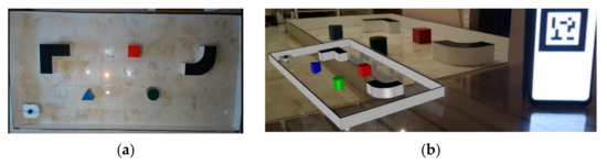
Additional collision checking is performed with obstacles belonging to the districts surrounding the district in which robot is currently positioned (due to the transition from one district to another). Typical robot surrounding real environment situation is shown in Figure 3. After each robot step, the environment is identified and detected by scanning with a laser range sensor. Augmented reality (AR) was used in experimental verification on a real polygon so that objects could be placed directly on the polygon, without the need for measurement. In the research, it was used as an aid in setting up a real polygon according to the 3D CAD model of the polygon, which was first modeled, and then used in the simulation.
The scanning process in the simulation is an adequate replacement for the LiDAR system on a real mobile robot system. The scanning process is defined with a minimal obstacle approach distance of 15 cm. The accuracy of the distance estimate depends on the actual distance. The closer the obstacle distance is, the estimate is more accurate and vice versa. In the same way, human estimates distance and produce estimation errors.
2.3. System Description
The main goal of the research presented in this paper is experimental checks, corrections, and adjustments of the used autonomous mobile robot’s behavior on the real polygon. Additionally, adjusting the real robot system’s behavior to match the virtual simulation robot’s model behavior is needed [30]. All the robot’s environment recognition and control algorithms were tested in the virtual reality software tool CoppeliaSim [31]. A virtual dynamic model of an eMIR (educational Mobile Intelligent Robot) mobile robot shown in Figure 4b and corresponding polygon configuration shown in Figure 5, are designed. Software support for constructing an experimental system is written in C++ programing language. By giving parameters and harmonizing these experiment outcomes, patterns and guidelines are provided for research, development and testing of algorithms for an autonomous cognitive behavior of mobile robot models in environments that do not have to be highly defined, for a much more comprehensive range of users, all with the aim of more effortless knowledge transfer [32].
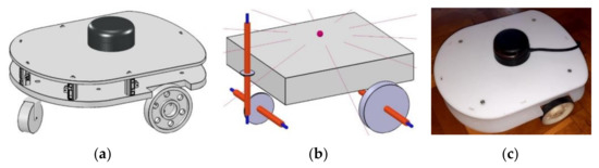
Figure 4.
Development of mobile robot educational Mobile Intelligent Robot (eMIR): (a) 3D Computer Aided Desing (CAD) model of eMIR; (b) dynamic model of eMIR (CoppeliaSim virtual reality simulator); (c) real mobile robot eMIR.
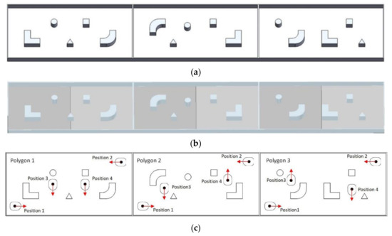
Figure 5.
Various polygon configurations: (a) 3D Computer Aided Design (CAD) models of three different polygon configurations for robot cognitive behavior training (b) models of three various polygon configurations constructed in CoppeliaSim, virtual reality software; (c) three various polygon configurations with four eMIR mobile robot starting positions that represent phases of learning, simulation and real experiment motion path.
The primary guideline of the proposed research in this paper is the development of a mobile robot behavior model that is entirely identical to the real system. The model is based on measurements. Within this research, the exploration of the environment by a mobile robot has been successfully conducted. The goal of building such a model is robot behavior ability to monitor lines on the polygon, plan the robot’s motion path in the model environment, and avoid obstacles on the polygon using range sensors installed on the mobile robot.
The proposed neuro-evolution learning is a cognitive navigation model that integrates cognitive mapping and the ability of episodic memory so that the robot can perform more versatile cognitive tasks. Three neural networks have been modelled for the construction of an environmental map. Neural networks have ten inputs representing laser range sensor beams (one beam every 36°). In two hidden layers, neural networks have 5, 10 or 15 neurons, with the corresponding biases. The neural networks also contain two outputs scaled to the mobile robot wheels velocities, described in Section 3. A system for storing and retrieving task-related information is also developed. Information between the cognitive map and the memory network is exchanged through appropriate encoding and decoding schemes. Neural network’s learning scores are tested in a simulation environment that is also developed in this research. The cognitive system is eventually applied to the real mobile robot’s system. Exploration, localization and navigation of the mobile robot are performed using this information data implementation. Real mobile robot experiments in the final experimental verification and validation proved the efficiency of the proposed system.
The proposed research uses the following materials and equipment:
- eMIR mobile robot of differential structure—is a mobile educational robot designed and built at the Faculty of Mechanical Engineering and Naval Architecture in Zagreb. It is equipped with an independent power supply, communication modules, camera module, range sensors and software interface. The eMIR is shown in Figure 1a. For this research, an additional mobile robot eMiR (white) has been made.
- A polygon with dimensions 2 × 4 m—an enclosed environment in which eMIR mobile robots perform various tasks. Environment floor and side walls are white to make the environment more vision system ready. There is the possibility to configure it with additional district/sector partitions if needed.
- The camera above the polygon—captures the tasks on a polygon, and it can calculate on the vision base robot’s position and orientation. The dynamics of the object tracking system is approximately ten calculations per second, which is quite sufficient, for the research purpose. The camera can also detect additional partitions because of its black coloured edges. The installed camera is not part of the control loop that controls the robot’s movement on the polygon (neither in the simulation nor in the real-world environment).
- Robot’s camera—captures the environment in front of the mobile robot. It has a 55° field of view, and object colour recognition can be done of the captured image. A separate software module processes the image and passes the recognition information to another module through a virtual communication channel. With the development of control algorithms accomplished in this research, this camera’s role in the system is minimized, so the camera is eventually excluded from the mobile robot’s control loop. Developed neural networks, supported by the developed genetic algorithms, solve a controlling process of mobile robot motion path successfully in learning, testing, and exploring a previously unknown environment. Of course, if it is an application of a mobile robot in the industry, the camera should be included in the control loop, for additional safety standards. It is necessary to have sensors on several levels and various detection systems. In case of failure of one level of operation, others remain functional.
- Robot’s laser range sensor (LiDAR)—in a simulation environment for the learning and testing data collection, LiDAR uses one detection laser beam on every 36° of a circular, horizontal pattern. This pattern and range are defined in CoppeliaSim virtual reality software. Full range sums a total of ten beams, as shown in Figure 6a. In the actual real-world system, developed for the research experiments, LiDAR operates on the same principles as in the simulation, as shown in Figure 6b.
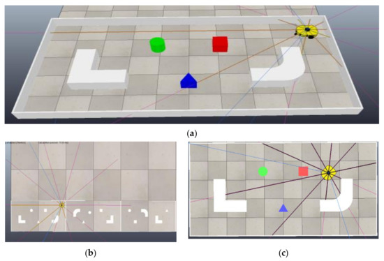 Figure 6. CoppeliaSim virtual reality polygons: (a) 3D side view of random polygon configurations with a mobile robot in motion; (b) stack of three various polygons made for mobile robot’s learning and training; (c) virtual reality polygon model with laser range sensor beams for detection of obstacles on every 36° pattern, identically configured as real polygon configuration shown in Figure 3a.
 - CoppeliaSim simulator (V-Rep)—is a virtual reality software with the possibility of many various robotic mechanism simulations that include dynamic properties. It has an integrated development environment, based on a distributed control architecture: each object/model can be individually controlled using a built-in script or custom software solution. It makes the simulator practised very versatile and ideal for multi-robotic applications. A robot’s and mechanism’s controllers can be written in several programing languages, such as C/C++, Python, Java, Lua, MatLab or Octave. It can be used as a standalone application or can be easily embedded in a user’s main application, as it has been done in this research. It has been used as a virtual simulation software platform in learning and testing process. Direct import of various 3D CAD models of polygons from any CAD software tool considerably advances model and configuration equivalence in the learning, testing and experimental validation on the real-world polygons. Augmented reality (AR), which is also used in this research, is also useful in making realistic models and experiment plans more intuitive.
- Qt Creator—an integrated development environment (IDE) with multiple platforms support. Supported platforms are Windows, Linux and macOS operating systems. In this research Qt Creator was used to develop software solutions for the neural networks and design of the graphic user interface for learning and training.
3. Mathematical Model of the Mobile Robot
The mathematical model of the robot’s non-holonomic differential drive with two drive wheels is described in this section. The analysis contains a kinematic interpretation of the entire system.
Model of the kinematics of a non-holonomic differential drive consisted of two wheels is illustrated in Figure 7, where:
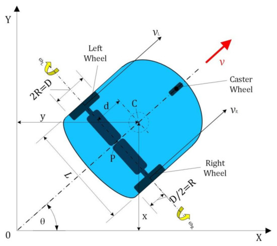
Figure 7.
Mobile robot’s kinematic model of the non-holonomic differential drive.
- L (m) is robot’s track width;
- R (m) is wheel radius;
- C is robot’s centre of mass (LiDAR’s centre of rotation);
- P is wheel’s axis middle point;
- d (m) is the distance between points P and C;
- (0, X, Y) is absolute coordinate system of a robot;
- (0, x, y) is relative coordinate system of a robot;
- θ (rad) is robot’s orientation to the X-axis;
- x (m), y (m), (rad) are parameters of the robot’s kinematics;
- (m/s), (m/s) are linear velocities of right and left wheel, respectively;
- (rad/s), (rad/s) are angular velocities of right and left wheel, respectively.
The non-holonomic implies that the robot does not have ability to move sideways, and motion is based on wheels angular movement principle [33]. Three parameters (x, y, θ) define the initial state of the mobile robot, which is represented with an equation q:
The kinematics model of a mobile robot is defined in matrix form as follows:
The kinematic model described by the previous equations is well known and can be found in the standard mobile robotics textbooks, e.g., [34].
4. Algorithms for Learning the Cognitive Behavior of the Mobile Robot eMIR
One of the applicable learning techniques in cognitive robotics is learning by knowledge acquisition. Learning by knowledge acquisition is one of the most complex learning techniques used for robot exploration of unknown space. In this paper, a neural network is used to guide the robot through unexplored space due to its ability to acquire knowledge in its weight coefficients. The learning process of a neural network using a simulated environment creates the knowledge needed for exploring unknown spaces of certain topology. Artificial neural network also has the ability to do the fusion of LiDAR data and give the robot motor angular velocities as the output. In this section the design and learning process of the neural network is explained.
4.1. Initialization of Neural Networks with Random Weight Coefficients
First, the initialization of neural networks with random weight coefficients at the first learning (zero generation) is described in Figure 8. The input of neural network contains ten values. These values represent obstacle distances, i.e., distance between objects placed in polygon and the eMIRs geometric centre of mass. Within the zero generation consisting of 100 population members, there are 100 neural networks with corresponding weight coefficients. A new neural network is generated with different randomly selected weight coefficients (red squares in Figure 8), for each population member. An example shown in Figure 8 describes one of the neural networks with corresponding zero generation. Initialization of this kind is used only during a zero generation. The network is populated with random numbers within interval −0.999 to 0.999. Lower interval limits were also tested. The result of using lower interval limits was slower robot’s learning and training of the neural network, which resulted in a low learning score (Section 7). This tests showed the robot’s inability to learn more complex movements, e.g., managing curves in a polygon, i.e., turning. It is a logical conclusion because fewer possible combinations are implemented, so the neural network output is repetitive at a higher rate (much less possible variations).
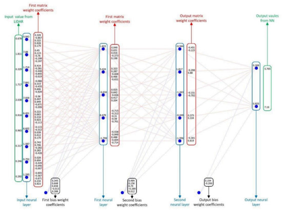
Figure 8.
Description of the neural network layers.
A detailed description of the neural network parts, i.e., the layers and weight coefficients is given in Figure 8. The neural network’s input neural contains ten values representing the detected distance from the LiDAR sensor (numerical values in the green frame). The same layer contains marked neural points (blue points in blue frame) where is the input activation function executed.
The most important thing that defines the ability of a robot’s “brain” is the number of weight coefficients in the neural network. That number directly affects its intelligence coefficient and the ability to solve problems and tasks. In detail, a description is given in Section 6. Results, where the impact of neural network dimension on the robot’s ability to solve a problem is shown.
The control neural network algorithm of eMIR uses obstacles distance values obtained by LiDAR as inputs in of neural network (Figure 9). The calculation with distance values is executed in each iteration of the program loop (frame). As a result of this calculation, the left and right eMIRs motor velocities are obtained. It is important to emphasize that within one simulation, i.e., one neural network, the weight coefficients always remain the same. Only neurons and neural network outputs are calculated. A mobile robot eMIR in the process of exploring a simulated environment is shown in Figure 6b.
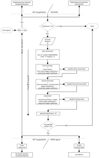
Figure 9.
Flow diagram of the neural networks algorithm.
4.2. Simulation and Neural Network Score Calculation
The first condition for simulation stop is a collision detection between eMIR and obstacles placed in the polygon. A second condition is reached iterations limit (specifically 1000 iterations). The last condition is when eMIR reaches maximum path distance. After stopping the robot’s movement, eMIR’s home position is initialized. The control neural network is evaluated, i.e., scored, by summing several parameters with an assigned specific coefficient (particular influence of individual scores on the total score): (a) exploration score of an environment; (b) wheels velocities; (c) difference in left and right wheel velocity; (d) simulation loops number; (e) eMIR’s distance reached; (f) an angle between the eMIR and free environment. The net score of particular neural network is calculated using formula:
where , , , are experimentally determined constants, is speed score, is difference score, is explored score, is loop score, is distance score, is angle score.
4.3. Generating a Neural Network
After the first population member in a generation, the second population member is generated, i.e., a new neural network. A new generated neural network is populated with new weight coefficients, which is repeated in cycles (Figure 10).
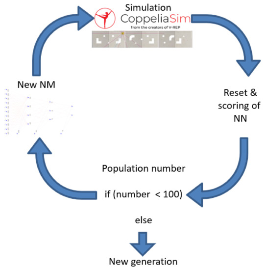
Figure 10.
Neural network generation cycle algorithm.
4.4. Completion of Zero Generation
For example, all of 100 population members were generated and simulated, indicating that zero generation is complete. Each of a population member corresponding neural network is assigned a certain number representing a calculated learning score for that network. The best and the second-best neural networks with their weight coefficients are selected from an entire generation. Follows the creation of a new generation by crossover and mutation processes.
4.5. Crossover Process
The first step towards new generation creation, i.e., the generation of a first population member within the first generation is the crossover process. Neural network from the previous generation with the first and second-best neural networks are mixed (Figure 11). More precisely said, weight coefficients are mixed in the ratio of “how much the first neural network is better than the second” in such a way that the weight coefficients from both networks are copied to the new empty neural network. A completion of the crossover process (mixing) generated a new neural network.
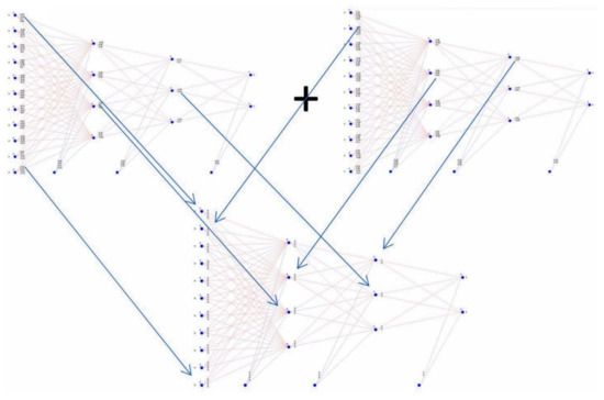
Figure 11.
Weight coefficients transfer to a new neural network (crossover process).
4.6. Mutation Process
A newly created neural network is forwarded to the mutation process (Figure 12). Randomly selected weight coefficients are overwritten with the new, randomly selected coefficients. The number of weight coefficients that are overwritten depends on the percentage of mutation. Crossover and mutation processes belong to genetic algorithms which can be thought of like Darwin’s theory of evolution simulation. The mutated neural network is “embedded” in the simulation is described in Section 4.1. The following steps are described in Section 4.1, Section 4.2 and Section 4.3, where the step described in Section 4.3. (Generating a new neural network), is replaced with the neural network generated by crossover and mutation product, described in Section 4.4. (Completion of zero generation), where the end of each subsequent generation is now defined. A new neural network is generated for each population member in this way (Figure 13). The best and second-best neural network are selected in the next generation as a continuously repeated cycle. Iterations of neural network generations indicate that eMIR is getting “smarter” and “solves the scenes (polygon)” in a more effective and faster way (Figure 14). Such cognitive learning of polygon solving process is stopped arbitrarily after adequate level of wanted eMIR’s behavior. An adequate level of behavior is usually stated when learning stagnation is occurred (scores do not change or change is negligible).
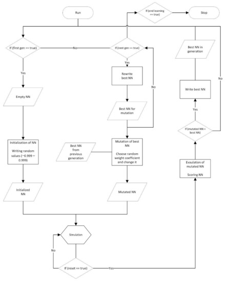
Figure 12.
Flow diagram of genetic algorithm.
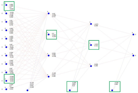
Figure 13.
The mutation process (the process of changing six random weight coefficients value).
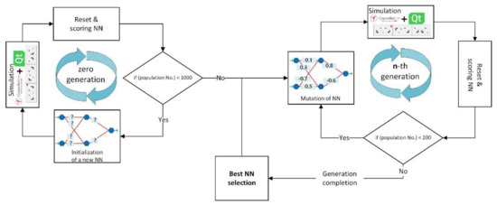
Figure 14.
Flow diagram of neural networks and genetic algorithms (neuro-evolution).
5. Cognitive Mechatronic System Design
Since the presented research system has obtained constructive results in the simulation tests, an actual mechatronic system was created. The new mechatronic system has an identical configuration and parts as the previous model used in simulation tests. This section describes the entire mechatronic system design, which consists of mechanical and electronic elements, developed software elements, vision and sensor systems, and a pool of computers for neural network learning and training process. The design of entire mechatronic system can be divided into three main steps: (i) design and training of neural network, (ii) virtual cognitive training, (iii) real-world cognitive test.
A topological view of the entire mechatronic system for constructing a cognitive model of a closed environment with a mobile robot’s use is shown in Figure 15.
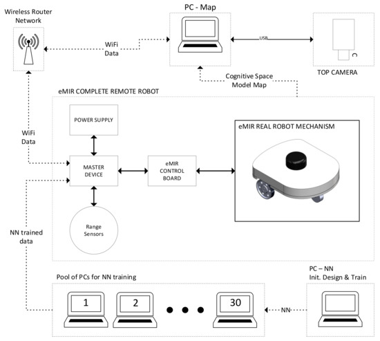
Figure 15.
Block diagram of the entire mechatronic system.
The entire learning and training process of eMIR’s behavior was initially executed on a single computer labelled PC-Neural Network (NN). Due to the learning process complexity, a very long execution time was needed. It was necessary to speed up the process several times, which was an impossible task due to all speed-up measures that had already been taken in the previous step. Therefore, a simultaneous learning and training process on the pool of computers is developed. The pool of computers consists of thirty personal computers usually available to the average user in terms of computational power. A first step in the learning and training process using the pool of computers was the initialization of neural networks on all computers. Thirty neural networks were created, and the best one with the best learning score was stated. Each subsequent learning and training iteration is initiated from starting “learning and training” point that is the previous best learned, trained and mutated neural network. Observing the learning score concludes which network is best learned and trained. Data values in the form of a textual file with numerical values are generated from the network with the best learning score. The neural network code is adapted to a mobile robot’s target master device computer (RaspberryPi; Linux; C programing language) installed on the mobile robot’s system.
The robot’s motion path description values are obtained by integrating control data used for drivetrain motors. The fusion of that data and distance data values obtained by LiDAR provided new data forwarded to a computer labelled PC-Map (Figure 15). Purpose of PC-Map computer is the environment data construction used for cognitive environment map modelling. The computer labelled PC-Map also has the task of capturing an image from a camera installed above polygon. The captured image is an aid for verifying mobile robot’s completed motion path, i.e., cognitive motion in an unknown environment. During its cognitive motion, mobile robot explores and maps unknown environment and various obstacles placed in it. The mobile robot is entirely autonomous and possibly needed data transfer between computer and master device on the robot itself is established in the local wireless network.
5.1. Mechanical Design of Mobile Robot
The following parameters describe the differential structure mobile robot’s mechanical characteristics used in the system. The mobile robot’s external dimensions are 300 × 250 mm (Figure 16). Mass of a robot with included sensors and power supplies is 3.15 kg. Drive wheels diameter is D = 80 mm. Distance between the drive wheels axis is L = 240 mm. Drivetrain motors gearboxes ratios are i = 71. On a previous mobile robot’s version, the gearboxes ratios were i = 27, which was not sufficient for this research experiments. A robot with gearbox ratio i = 27 had higher velocity at the same motor revolutions value (same voltage). The undesired property also was motion responses to control values obtained from neural networks that were too rough, i.e., the robot did not move smoothly and without jerking. The maximum rotational wheels velocity while the motors are supplied with the highest rated voltage of 12 V, is approximately , i.e., . Motors gearboxes with a lower gear ratio had higher wheels velocity of , i.e., . A given velocity generates 364 pulses per second on the encoder output. The maximum translation velocity of the mobile robot is vmax = 185 mm/s (lower gearbox ratios generated vmax = 500 mm/s). The maximum rotational speed of the mobile robot is ωmax = 90 °/s (lower gearbox ratio generated ωmax = 240 °/s).
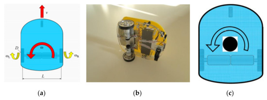
Figure 16.
eMIR-mobile robot of differential kinematic structure: (a) Kinematic values; (b) Real mobile robot’s drivetrain; (c) LiDAR’s position on a mobile robot and its rotation direction (point C on Figure 7).
The polygon elements are shown in Figure 4, in Section 2. The polygon dimensions are 4 × 2 m, with a maximum height of all elements 200 mm. Dimensions of particular obstacles are not exceeding 500 × 500 mm. The ratio of the mobile robot’s dimensions and the polygon within the CAD model (scale 1:1) is shown in Figure 3a.
5.2. Electronic Design of Mobile Robot
The mobile robot is the main subject of the system to explore the unknown environment and generate the data needed to create a cognitive map of the unknown space. Figure 17 shows a block diagram of the electronic system of the mobile robot. The primary control device or master device is an SoC card computer (RaspberryPi 4B), based on the Linux operating system. A distance of the obstacles in an unknown environment is obtained with a single laser range sensor (LiDAR, model RPLIDAR A2). The mobile robot is driven by two DC motors operating in differential mode. Output torque is multiplicated by gearboxes attached to the drivetrain motors. Power signal for motors is generated by motor drivers (H-bridge electronic circuit, LMD18200T). Each motor has its driver. The driver control signal from the master device is generated on the GPIO port. A control signal type is the Pulse Width Modulated signal (PWM). Two independent battery supplies powers the entire robot’s system with a common ground terminal. The first power supply is a battery power bank for master device and LiDAR supply to ensure the voltage stability required for electronic components with a rated voltage of 5 VDC. Drivetrain (motors and drivers) have a separate battery power supply of higher capacity that can withstand higher draw currents. The main goal in the process of power supply selection was a more extended mobile robot’s autonomy.
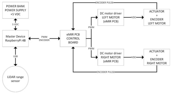
Figure 17.
Block diagram of a mobile robot’s electronic system.
5.2.1. Master Device of Mobile Robot
For the role of the master device, a SoC card computer RaspberryPi 4B was selected. Small dimensions are useful in this application due to the increased need for mobility of the robot and its independent (autonomous) operation in unknown, unexplored environments. The computer’s relatively high processing power specification is useful for the fast control parameters calculations using neural networks. Additionally, processing large amounts of environment data obtained using LiDAR sensors is done fast enough.
5.2.2. Laser Range Sensor for Environment Exploration
A two-dimensional laser range sensor with a 360-degree detection angle is shown in Figure 18. The number of samples per second is up to 8000 samples. A large number of samples in one second is possible due to the laser transmitter and receiver part’s high rotational speed. A selected LiDAR can scan the environment in two dimensions. An obstacle placed in an environment can be detected in all directions if it is not exceeding the detection range of 12 m. It is possible to extend detection range to 18 m with the adjustment of the control software. The data from sensor output is in the form of points with two-dimensional coordinates. Generated data is used to map and model objects placed in an unknown environment where the robot is exploring. LiDAR system connected to a data transfer interface provides information about the environment. The RPLIDAR A2 laser range sensor’s rated scanning frequency is 10 Hz, which corresponds to 600 rpm. The actual scanning frequency can be adjusted according to the application needs in the range of 5 to 15 Hz. The laser range sensor uses the laser triangulation method. Use of laser range sensor adds exceptional detection performance in systems for various indoor and outdoor environments, without the external parameters which obstruct detection performance (e.g., sunlight).
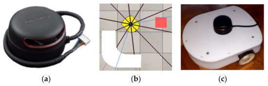
Figure 18.
LiDAR in mobile robot’s system: (a) RPLIDAR A2 device; (b) simulation model of LiDAR device (CoppeliaSim; one beam every 36°); (c) RPLIDAR A2 device installed on eMIR.
5.2.3. Drivetrain and Power Supply
A power bank with a capacity of 10,000 mAh was used to power the master device and LiDAR on a mobile robot. The second battery of 5000 mAh capacity was used to power the drivetrain elements (DC electric motors and driver). The control PCB system also contains a step-down voltage converter, so it is possible to reduce the system to a single power source. DC electric motors with brushes model IG320071×0014 were used for a mobile robot’s movement. The rated voltage of motors is 6 to 24 VDC. A maximum rated speed of 1000 rpm is reached at 200 mA draw current. An encoder is attached to the motor housing to detect the angular position and the motor’s number of revolutions. A gearbox is attached to the motor’s output shaft to increase the motor’s torque on the output shaft. LMD18200T drivers were used to modulate control signal to power and control DC motors. The maximum driver output current is 3 A, selected to match the electric motor demand. The control signal generated by the master device hardware PWM unit has a frequency of 330 kHz and the modulated duty cycle range. The electric motor’s rotational velocity is controlled by the modulated duty cycle of a PWM signal. The experimental tests concluded that the motors have an insufficient output torque if the duty cycle is less than 30%. Therefore, the electric motor’s angular velocity is controlled by a duty cycle modulation range of 30% to 100%, so that minimal torque needed for the robot’s movement is present. The PWM signal generated by the hardware PWM unit of a master device is forwarded to the GPIO port of a master device, directly wired to the motor drivers input. There is a need for an electric motor’s rotation direction control, which these drivers also support.
5.3. System Software Development
The development process of the final cognitive model map of an unknown environment is shown in Figure 19 as blocks in chronological order. Below is a more detailed description of each section.
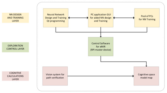
Figure 19.
Software development block diagram.
5.3.1. Design and Training of Neural Network Software
Neural networks and genetic algorithms were written in the C ++ programing language, using a Qt Creator IDE software tool. Code is written “from scratch”, i.e., that libraries like TensorFlow [35] or Keras [36] were not used at all. Mentioned libraries are also the most popular selection in artificial intelligence development. A programing approach “from scratch” is used for establishing insight into each part of the neural network and possibility of modifying each part due to the specific problems that the artificial intelligence must solve in the proposed hypothesis.
5.3.2. PC Application for Neural Network Control and Data Collection (GUI)
The GUI has three operation modes selected with a button in the upper left corner of the program window (Figure 20). The first mode of operation is labelled “New”. It is a mode of operation in which learning starts from zero, i.e., learning begins by generating random weight coefficients. The second mode of operation is labelled “Continue”, and it is a mode in which the learning of a previously learned neural network continues. Furthermore, the third mode of operation is labelled “One Run”. It is an operation mode used for results validation or to simulate eMIR’s movement in an unknown environment after previously learned neural network. This mode represents a mobile robot’s commissioning in a real-world environment. Connection to the CoppeliaSim simulation software is initialized by a button placed in GUI.
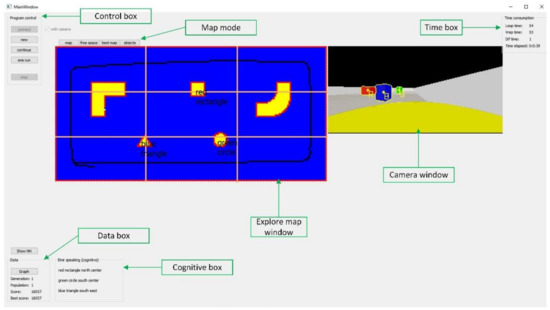
Figure 20.
PC application for Neural Network (NN) control and data collection.
Furthermore, the GUI window centre has placed a subwindow for presenting the environment already explored with eMIR. This subwindow consists of a 200 × 100 pixel map, i.e., a scaled polygon environment of 400 × 200 cm. It implicates the fact that the entire system is mapped with a resolution of 2 cm. A time interval data is shown in the upper right corner of the main GUI window. The time required for the application and simulation to calculate one simulation step is displayed. There is also the difference between these two speeds displayed, since the calculation time of one step of CoppeliaSim is always longer. The current generation, learning score obtained in the previous population member, and the best learning score obtained in an entire generation are also displayed in GUI. The buttons for presenting and exporting trends are also placed in this part of the GUI. After each generation, trends are generated with all individual learning scores and the best score of neural network learning in the entire generation. It is possible to visualize an entire neural network in real-time with the dedicated button. The neural network’s inputs and outputs, weight functions, and the neuron’s value for each layer of the neural network are visualized in this subwindow.
5.3.3. Mobile Robot’s Control Software
Part of the neural network algorithms related to the feedforward calculation of the neural network’s output is programed in eMIR’s master device (RaspberryPi 4B). When is the environment exploration requested, i.e., when eMIR starts to explore, the weight coefficients are imported to the application from the text files. The weight coefficients resulted from eMIRs learning and training on polygons within the simulation. The coefficients were transferred to the master device computer after eMIR’s behavior gained an acceptable level and after neural network reached a satisfactory score. The neural network’s calculation begins with imported weight coefficients, as shown in the flow diagram of a neural networks algorithm in Figure 9. The same algorithm is used in the simulation. The only difference is that actual distance values from LiDAR are used for the neural network’s input. It is important to note that these values have the same distance unit (meters), only they are obtained from another source. Likewise, the outputs are scaled to a duty cycle of the PWM signal. So, values from 0 to 10 must be scaled to values 0 to 1023, as it is the range of 10-bit PWM used for eMIR’s movement control. The scaling is only mathematical, and there is no other operation on values obtained from the neural network’s output. No other control logic is used for the eMIR’s movement control. The only part of the neural network that differs from the simulation is shown in Figure 9 (right lower and upper part of a figure). It is proof for one of the main hypotheses of this research, declaring that it is possible to use identical algorithms in the simulation as in the real world. The direct transfer of the weight coefficients from the simulation part to the real mobile robot is proof of a hypothesis, as eMIR behaves “identically” as in the simulation. Only minor adjustments in the already mentioned neural network’s input and output part is needed, that does not interfere with a hypothesis statement. Now it is shown that there is a minimal difference between simulated and real systems. The eMIR can be learned in a brief time interval because only step to do is transferring the already mentioned “learned” weight coefficients and execute a request for exploration which will be done as it was done in simulation. With this approach, various tests can be performed. More complex learning and training processes can be performed, which is seen as a logical extension of this research, using the proved hypothesis of “identical” behavior between simulated and real systems.
5.3.4. Vision System for Path Verification
Logitech C920 webcam is installed above the polygon (Figure 21). The camera is used to capture a mobile robot’s movement in the process of exploration of an unknown environment, in this case, a polygon. The camera virtually installed in CoppeliaSim simulator has the role of motion tracking of a virtual mobile robot in a virtual environment. In the real system, a camera’s role is a mobile robot’s motion path verification, relative to the motion path obtained in the simulation. In path verification tests, a mobile robot had a bag of sand attached to its housing, leaving a visible path mark on the polygon’s surface. Since the use of sand is not a practical solution, a software solution was developed. The motion of the mobile robot’s geometric centre of gravity was drawn in path image. Centre of geometric gravity was attached in the centre of laser range sensor.
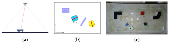
Figure 21.
Vision system for path verification: (a) camera’s position above the polygon; (b) position and orientation of the absolute coordinate system; (c) mobile robot’s path drawn on the image captured by the camera.
5.3.5. Cognitive Environment Model Map Construction
Based on the kinematics model of the mobile robot presented in Section 3 it is possible to construct algorithm for the cognitive map of a mobile robot’s environment. Defined algorithm is used for constructing cognitive map of an unknown environment where robot is placed for exploring. The cognitive map of the mobile robot’s closed environment based on measurements is constructed, and it is the only part of an entire cognitive model of the closed environment. The information about the environment obtained from the cognitive map is base for planning an optimal mobile robot’s motion path. A high level of the environment information, close to human perception abilities, are established using the obtained cognitive map. The first hypothesis of the main contributions of the proposed research was proven. At the end of a mobile robot’s exploration process, a list of cognitive information about the environment is established. The polygon’s configuration is obtained using that list of information, from a room’s entrance (polygon starting point) to the relative point in which robot achieved good enough exploration score. The fusion of the LiDAR and integrated motor control signal information was used for the cognitive map construction, as shown in Figure 22a.
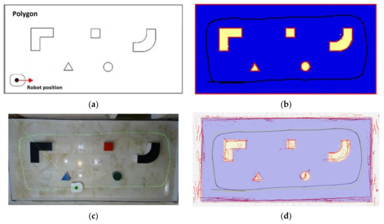
Figure 22.
Environment cognitive model map: (a) selected polygon configuration; (b) map of the polygon obtained by simulation; (c) real-world experiment on the real polygon with tracked robot’s motion path; (d) closed space map obtained by fusion of robot sensors readings, base for building of cognitive map; (e) interpretation of the obtained (by mobile robot’s ability for cognitive exploration) high-level information about a previously unknown environment.
Map of an unknown environment is constructed without any pre-defined real-world information, i.e., an environment has not been previously known to the robot. The cognitive map of environment is constructed from the results presented in Figure 22b–d. These intermediate result obtained by fusion of readings from robots LiDAR and odometry are passed to another pattern search algorithm that finds objects and positions of their centroids. The positions of the centroids are then classified according to regions shown in Figure 22e. Detected objects have to be classified according to their geometrical features. For this classification, a simple algorithm is designed. Using OpenCV functions on the intermediate results from Figure 22d the bounding boxes are formed around any detected object and surface area of the object is measured. Classification is achieved by the comparison of bounding box surface area Abb and surface area of the object Aobj. The ratio of surface areas of the bounding box and object for each object used in the experiment are presented in Table 1.

Table 1.
Surface area ratio used for object classification.
Due to noise in the sensor measurements, the objects are classified using presented ratio ranges. If mentioned ratio falls outside all ranges, the object is classified as “unknown“. After the classification, a cognitive map of closed environment is produced. The cognitive map is presented by the literal explanation of the object positions in the explored space, e.g., “Blue triangle SW“ or “Green circle south center“. The results are shown in Figure 22e.
The built cognitive map advances the mobile robot’s abilities for “conversation with humans”, i.e., establishing communication with a human on a high-level information exchange as the human perception. Cognitive information exchange obtained by eMIR is shown in Figure 22e. If the information about an environment has been collected in a pre-defined knowledge database, then the mobile robot’s would not be “cognitive”, i.e., its abilities would be reduced as it could not be able to explore in non-described environments that are not included in the knowledge database. In the exploration process, a mobile robot must obtain knowledge about an environment in which is placed, i.e., it must obtain human-understandable information about an environment around it. One real-world-human scenario is when a human enters an unknown room or environment (e.g., polygon in Figure 22a, dimension 4 × 2 m). Only knowledge that he has at that moment is steps, an exploration time, an approximate positions and orientations of objects and obstacles placed in that environment, a correlation between objects, obstacles and walls (dimension of the polygon or room), and a correlation between objects itself.
5.4. Pool of Computers System
The pool of computers system’s topology for neural network learning and training is shown in a block diagram in Figure 23. The main part of the system is the master computer with installed Veyon Master software package, while on the other thirty computers is installed Veyon Slave software module (Figure 24). Computers are in a local network over the network switch, connected to the Internet via a server. The master computer has TeamViewer software installed for remote access, which gives the advantage of remote access to the pool of computers. The system can be monitored from any location in real-time, which allows controlling the neural network’s learning and training process. It also enables monitoring of the neural network learning score, and whether it is advancing towards the expected trend. It is essential to mention that this is a low-cost solution because of used personal computers accessible by an average user. In future research, the authors considered creating an algorithm that will automatize neural network learning and training. An automated process is planned to work as follows: thirty computers will advance into new learning iteration from the point obtained neural network, which has gained the highest learning score in the previous iteration. An algorithm would transfer this neural network to the remaining twenty-nine computers to further learning process. After completing the desired goal (neural network learning score or time interval), a master computer will forward the learned data to a remote computer via the Internet.
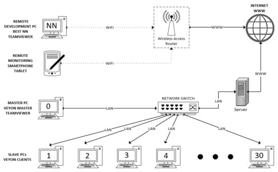
Figure 23.
The pool of computers used for NN learning and training.
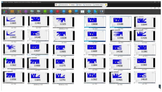
Figure 24.
Pool of computers remote control interface (Veyon software).
6. Results
After completed exploration of an environment, the eMIR is placed in the home position. The neural network used to control eMIR’s motion path is scored in the form of a several parameters sum:
- Environment exploration percentage;
- Wheels velocities;
- The velocity difference between wheels;
- Number of simulation iterations;
- eMIR’s total distance reached;
- The angle between eMIR and free environment.
The total score reached during the learning process of various neural networks with various input functions is shown in Figure 25 (Linear shape) and Figure 26 (Sigmoid shape). The data collection is stopped when there is no visible progress in the neural network learning process. Stagnation in the learning process can be seen from the trends where rising trend straightens up to a horizontal line or in some cases, the line gets a decreasing trend, i.e., score starts to decrease. The expected score number is approximately 16,000, which also stands for the maximum score. This number is impossible to determine precisely due to the very nature of learning by neural evolution.
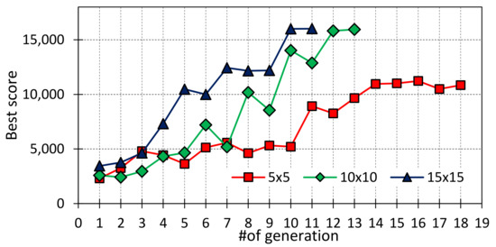
Figure 25.
Score through the neural network generations (Linear shape).
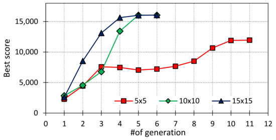
Figure 26.
Score through the neural network generations (Sigmoid shape).
The chart shows that the activation function with Sigmoid shape gives better learning score outcomes. The curve is steeper for the lesser number of generations, compared to the other activation functions. It is proof of the statement: it is essential for a robot to know an entire environment, regardless of the travelled distance, to perceive the world fully and accurate. With this activation function (more detailed description is in Section 7), an influence of obstacle on the robot, rises logarithmically with obstacle being closer to the robot. In comparison, the second activation function has much worse results. It describes this distance linearly and only in the local environment where the robot is placed.
If both activation functions are tested in the correlation with the dimension of the neural networks, better scores are gained by a higher dimension neural networks. It gained a higher score, but this is done in a narrower time interval with fewer generations. Use of the more complex networks and input functions covering full distance results in faster learning is shown in these two learning process segments.
A given outcome is expected because a larger neural network will be able to solve a more complex scene (obtain a higher score in less time). A larger neural network have many more possible combinations and with given input values, generates a greater number of possible neural network outputs.
Starting assumption was that a larger neural network would need more time for the learning process due to more possible combinations that should be reached within a mutation process, but the research showed the exact opposite.
Although there is a higher number of weight coefficients, it would take more mutations and generations to achieve an appropriate set of weight coefficients for an acceptable neural network’s performance.
It was found that a larger neural network implicates many more acceptable combinations at a much higher learning rate.
This part of the research showed the minimal neural network dimensions sufficient for solving an assigned scene or task.
Comparison of Mobile Robot’s Motion Paths
Mobile robot behavior during the exploration of the environment and its motion path is described in this section. Comparison of the motion path of the real robot and motion path of the robot’s model in simulation showed that real mobile robot succeeded in an attempt to explore an environment as it has done in simulation. Motion paths were approximately the same, which is also proof of the stated hypothesis.
7. Discussion
Research has shown that mobile robot controlled by a 5 × 5 neural network has poor movement performance, as it tends to the linear description of a motion path (Figure 27).
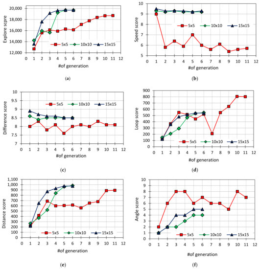
Figure 27.
Neural network learning results through the neural network generations: (a) exploration score; (b) speed score (velocity coefficient); (c) difference score (velocity difference); (d) loop score (number of iterations); (e) distance score (distance reached); (f) angle score (angle between eMIR and free environment).
A learning phase in the simulation showed that a mobile robot tends to circular motion paths, driven by the assumption that a smaller neural network will have a more linear motion path.
The activation functions
where x represents the robot distance from an obstacle are the excellent starting point for continued research.
This research emphasizes the possibility of a mobile robot’s behavior in new unknown environments, with high state of similarity to human behavior in the same conditions of environments. The same is proven with conducted experiments.
Reviewing papers about neuroevolution in mobile robotics, the exact parameters of neural networks and genetic algorithms were not mentioned. It means that there is no reference to an activation function, neural network scoring methods, population numbers in one generation and mutation percentages, which all were used in this research. This research also shows how increasing or decreasing neural networks affects the speed and quality of neural networks learning and training process.
The activation Equation (6), has much more aggressive response at distances up to 2 m, i.e., that the derivation (or change) is closer to 0. At distances of 2 m and further, activation function has a very mild response, and it asymptotically approaches the value of 8.
The activation Equation (7) is a linear function that multiplies the input by 7, within range of 1 m. The function rounds all greater distances than 1 m to a value of 7, i.e., a function is saturated above 1 m. With the activation function, the mobile robot’s local environment within a radius of 1 m is described. The perimeter is placed around a mobile robot’s current location, where is a need for robot behavior verification in correlation to its environment with included obstacles and limits. The mobile robot (neural network control algorithm) will not react to values further (larger) than 1 m. The mobile robot’s exploration motion path used for the testing are shown in Figure 28.
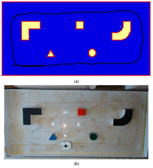
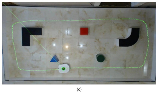
Figure 28.
Mobile robot’s exploration motion path: (a) cognitive model map with robots motion path; (b) motion path of a real robot (sand trace); (c) motion path of a real robot (software drawn in captured image from a camera).
Before aiming for future research, it should first be mentioned that the research has been proven to reduce the gap between the simulated and the real movements of mobile robots in unknown environments. One of the guidelines was that all simulations, learning and testing processes and real system experiments are carried out on equipment easily available to the average user. Guided by these constraints, the authors propose increasing the polygon dimensions for experiments and more complex environments similar to those surrounding humans. That implicates using more advanced range sensors capable of detection, classification and cognitive perception of the more complex environments. Sensors must be thought of as an information collecting device, that forwards collected information to developed neural networks, i.e., mobile robots. The described experiments require more powerful computers for the learning, simulation and interpretation of learned knowledge on real mobile robots. However, it should be noted that a computer RaspberryPi 4B used in this research has its limitations for more complex tasks.
8. Conclusions
This research’s primary hypothesis has been to prove the mobile robot’s ability to map an unknown environment using neural networks as control algorithms. The “brain” in human cognitive language terms or master device in terms of mobile robot parts has been learned and trained by neuroevolution. Simulation in which neuroevolution has been established represents real conditions and many more world possibilities than the real experiment, including real robot system. The ability to increase a simulation execution time is also possible, i.e., it is possible to gain higher learning speed than it is possible in the real world. Experiments presented in this research would be nearly impossible to conduct in real-world systems because the learning and training process would take a very long time. The trained “brain” with gained knowledge has been transferred to the real mobile robot’s system, indicating possible applications in real-life situations.
The research methodology contains the definition, analysis and establishment of an acceptable interactive cognitive model of the closed environment of a mobile robot. Validation and verification of the model were performed through a series of simulations of simpler straightforward problems. The entire model of interaction between the mobile robot and the environment was gradually defined. The cognitive environment model is constructed with the fusion of the mobile robot’s position and orientation data, a distance of obstacles in polygon data collected by LiDAR on the robot and data about motion path integrated from the encoders attached to the robot motors. The research hypothesis and statements were tested on a real system consisting of a mobile robot and a polygon, equipped with range sensors and vision path verification system. The correlation between the obtained information resulted in new information. After completing the initial request to explore an unknown environment, the mobile robot uses this newly obtained information to describe a now known environment. The description consists of basic cognitive language elements, with no precisely defined measurement elements like distance or position in the coordinate system in the environment. A description is focused on the location of elements in the environment and what they look like, according to learned data (refer to Supplementary Materials).
In summary, the main contributions of this research are listed as follows:
- (1)
- By fusing various types of data from various sources in order to construct more complex information suitable for constructing a cognitive model of the closed environment of a mobile robot, a trustworthy simulation-real model (STR) has been established.
- (2)
- A selection of information and methods for constructing an environment model used for real-time applications has been defined.
- (3)
- A cognitive model of the closed environment of a mobile robot that is directly applicable in real-world scenarios without any predefined real-world data has been constructed.
- (4)
- Experimental verification and validation of the constructed cognitive model of the closed environment of a mobile robot has been established in a real polygon with a real mobile robot system, and it has been successful in the full extent of hypothesis.
Supplementary Materials
Materials such as programing code, algorithms, CAD models and other research materials are available online at: https://drive.google.com/drive/folders/1Td0qQYwubNo5B3O35yM-nev2KvcnmCWm?usp=sharing (accessed on 18 March 2021). Video presentation of entire research is available at: https://www.youtube.com/watch?v=KUxVIAe8hSM (accessed on 18 March 2021).
Author Contributions
Conceptualization, T.P., K.K., D.R., V.M. and M.C.; formal analysis, T.P., K.K., D.R., A.B., M.L. and M.C.; methodology, T.P. and M.C.; project administration, T.P. and V.M.; software, T.P., K.K., D.R. and A.B.; supervision, V.M. and M.C. All authors have read and agreed to the published version of the manuscript.
Funding
Research was founded entirely by authors.
Institutional Review Board Statement
Not Applicable.
Informed Consent Statement
Not Applicable.
Data Availability Statement
Data is contained within the article or Supplementary Materials.
Conflicts of Interest
The authors declare no conflict of interest.
Abbreviations
The following abbreviations are used in this manuscript:
| AI | Artificial Intelligence |
| eMIR | educational Mobile Intelligent Researcher |
| SLAM | Simultaneous Localization And Mapping |
| DRL | Deep Reinforcement Learning |
| STR | Sim-To-Real |
| RPi | Raspberry Pi |
| CAD | Computer Aided Design |
| CAM | Computer Aided Manufacturingcam |
| CNC | Computer Numerical Control |
| NN | Neural Network |
| GA | Genethic Algorithm |
| AR | Augmented Reality |
| GUI | Graphics User Interface |
| GPIO | General-purpose input/output |
| PWM | Pulse-width modulation |
| LiDAR | Light Detection and Ranging |
| SoC | System on a Chip |
| IDE | Integrated Development Environment |
| IKP | Inverse Kinematic Problem |
References
- Liu, N.; Lu, T.; Cai, Y.; Wang, S. A Review of Robot Manipulation Skills Learning Methods. Acta Autom. Sin. 2019, 45, 458–470. [Google Scholar]
- Karkalos, N.E.; Efkolidis, N.; Kyratsis, P.; Markopoulos, A.P. A Comparative Study between Regression and Neural Networks for Modeling Al6082-T6 Alloy Drilling. Machines 2019, 7, 13. [Google Scholar] [CrossRef]
- Liu, N.; Lu, T.; Cai, Y.; Wang, R.; Wang, S. Real-world Robot Reaching Skill Learning Based on Deep Reinforcement Learning. In Proceedings of the Chinese Control and Decision Conference (CCDC), Hefei, China, 22–24 August 2020. [Google Scholar]
- Liu, N.; Cai, Y.; Lu, T.; Wang, R.; Wang, S. Real–Sim–Real Transfer for Real-World Robot Control Policy Learning with Deep Reinforcement Learning. Appl. Sci. 2020, 10, 1555. [Google Scholar] [CrossRef]
- Thomas, A.; Hedley, J. FumeBot: A Deep Convolutional Neural Network Controlled Robot. Robotics 2019, 8, 62. [Google Scholar] [CrossRef]
- Wang, H.; Guo, D.; Liang, X. Adaptive vision-based leader-follower formation control of mobile robots. IEEE Trans. Industr. Elect. 2017, 64, 2893–2902. [Google Scholar] [CrossRef]
- Liu, M. Robotic online path planning on point cloud. IEEE Trans. Cyber. 2016, 46, 1217–1228. [Google Scholar] [CrossRef] [PubMed]
- Szegedy, C.; Liu, W.; Jia, Y.; Sermanet, P.; Reed, S.; Anguelov, D.; Erhan, D.; Vanhoucke, V.; Rabinovich, A. Going Deeper with Convolutions. In Proceedings of the 2015 IEEE Conference on Computer Vision and Pattern Recognition (CVPR), Boston, MA, USA, 7–12 June 2015; pp. 1–9. [Google Scholar]
- Crneković, M.; Sučević, M.; Brezak, D.; Kasać, J. Cognitive Robotics and Robot Path Planning. In Proceedings of the CIM05-International Scientific Conference on Production Engineering, Lumbarda, Korčula, Croatia, 15–17 June 2005. [Google Scholar]
- Crneković, M.; Zorc, D.; Sučević, M. Cognitive Model of Mobile Robot Workspace. In Proceedings of the CIM07—Computer Integrated Manufacturing and High Speed Machining, Biograd, Croatia, 13–17 June 2007; pp. 95–102. [Google Scholar]
- Crneković, M.; Zorc, D.; Kunica, Z. Research of Mobile Robot Behavior with eMIR. In Proceedings of the International Conference on Innovative Technologies, Rijeka, Croatia, 26–28 September 2012. [Google Scholar]
- Crneković, M.; Zorc, D.; Kunica, Z. Mobile Robot Vision System for Object Color Tracking. In Proceedings of the CIM2013 -Computer Integrated Manufacturing and High Speed Machining, Biograd, Croatia, 19–22 June 2013; pp. 93–98. [Google Scholar]
- Crneković, M.; Pavlic, T.; Lukas, M. Programming Language for the eMIR Mobile Robot. In Proceedings of the 15th International Scientific Conference on Production Engineering, Vodice, Hrvatska, 10–13 June 2015; pp. 81–89. [Google Scholar]
- Pavlic, T.; Lukas, M.; Crneković, M. Design and Control of Robotic Arm for Educational Mobile Robot. In Proceedings of the 15th International Scientific Conference on Production Engineering, Vodice, Hrvatska, 10–13 June 2015; pp. 207–211. [Google Scholar]
- Malayjerdi, E.; Yaghoobi, M.; Kardan, M. Mobile robot Navigation Based on Fuzzy Cognitive Map Optimized with Grey Wolf Optimization Algorithm used in Augmented Reality. In Proceedings of the 2017 5th RSI International Conference on Robotics and Mechatronics (ICRoM), Tehran, Iran, 25–27 October 2017. [Google Scholar]
- Richter, C.; Roy, N. Safe Visual Navigation via Deep Learning and Novelty Detection. Robot. Sci. Syst. 2017. [Google Scholar] [CrossRef]
- Stückler, J.; Schwarz, M.; Behnke, S. Mobile Manipulation, Tool Use, and Intuitive Interaction for Cognitive Service Robot Cosero. Front. Robot. Ai 2016, 3, 58. [Google Scholar] [CrossRef]
- Bijo, S.; Pinhas, B.T. Physics Based Path Planning for Autonomous Tracked Vehicle in Challenging Terrain. J. Intell. Robot. Syst. 2018, 95, 511–526. [Google Scholar]
- Armesto, P.; Fuentes-Dur’a, P.; Perry, D. Low-cost Printable Robots in Education. J. Intell. Robot. Syst. 2015, 81, 5–24. [Google Scholar] [CrossRef]
- Farías, G.; Fabregas, E.; Peralta, E.; Torres, E.; Dormido, S. A Khepera IV library for robotic control education using V-REP. Ifac-Pap. 2017, 50, 9150–9155. [Google Scholar] [CrossRef]
- Tai, L.; Giuseppe, P.; Liu, M. Virtual-to-real Deep Reinforcement Learning: Continuous Control of Mobile Robots for Mapless Navigation. In Proceedings of the 2017 IEEE/RSJ International Conference on Intelligent Robots and Systems (IROS), Vancouver, BC, Canada, 24–28 September 2017. [Google Scholar]
- Becker, T.; Alberto Fabro, J.; Schneider de Oliveira, A.; Reis, L.P. Adding Conscious Aspects in Virtual Robot Navigation through Baars-Franklin’s Cognitive Architecture. In Proceedings of the 2015 IEEE International Conference on Autonomous Robot Systems and Competitions, Vila Real, Portugal, 8–10 April 2015. [Google Scholar]
- Jiménez, A.C.; García-Díaz, V.; Bolaños, S. A Decentralized Framework for Multi-Agent Robotic Systems. Sensors 2018, 18, 417. [Google Scholar] [CrossRef] [PubMed]
- Heng, L.; Gotovos, A.; Krause, A.; Pollefeys, M. Efficient Visual Exploration and Coverage with a Micro Aerial Vehicle in Unknown Environments. In Proceedings of the 2015 IEEE International Conference on Robotics and Automation (ICRA), Seattle, WA, USA, 26–30 May 2015. [Google Scholar]
- Båberg, F.; Wang, Y.; Caccamo, S.; Ögren, P. Adaptive Object Centered Teleoperation Control of a Mobile Manipulator. In Proceedings of the 2016 IEEE International Conference on Robotics and Automation (ICRA), Stockholm, Sweden, 16–21 May 2016; pp. 455–461. [Google Scholar]
- Hossein Ghaffari, N.; Peixoto, N. Assessment of Evolutionary Processes Experiments on Self-Organizing Behavior of E-pucks. In Proceedings of the 2016 IEEE Symposium Series on Computational Intelligence (SSCI), Athens, Greece, 6–9 December 2016. [Google Scholar]
- Ciszewski, M.; Mitka, Ł.; Buratowski, T.; Giergiel, M. Modeling and simulation of a tracked mobile inspection robot in MATLAB and V-REP software. J. Autom. Mob. Robot. Intell. Syst. 2017, 11, 5–11. [Google Scholar] [CrossRef]
- Nagy, Á.; Csorvási, G.; Kiss, D. Path Planning and Control of Differential and Car-Like Robots in Narrow Environments. In Proceedings of the 2015 IEEE 13th International Symposium on Applied Machine Intelligence and Informatics (SAMI), Herl’any, Slovakia, 22–24 January 2015. [Google Scholar]
- Ivaldi, S.; Padois, V.; Nori, F. Tools for dynamics simulation of robots: A survey based on user feedback. arXiv 2014, arXiv:1402.7050. [Google Scholar]
- Cognitive Model of the Closed Environment of a Mobile Robot Based on Measurements. Available online: https://www.youtube.com/watch?v=KUxVIAe8hSM (accessed on 14 February 2021).
- Cognitive Mobile Robot Design. Available online: https://youtu.be/x7lF3olP7Kw?t=21 (accessed on 14 February 2021).
- Stengel, R.F. Robotics and Intelligent Systems—A Virtual Reference Book; Princeton University: Princeton, NJ, USA, 2017; Available online: http://www.stengel.mycpanel.princeton.edu/RISVirText.html (accessed on 14 February 2021).
- Lucas, G.W. A Tutorial and Elementary Trajectory Model for the Differential Steering System of Robot Wheel Actuators. Available online: http://rossum.sourceforge.net/papers/DiffSteer/ (accessed on 14 February 2021).
- Siegwart, R.; Nourbakhsh, I.R. Introduction to Autonomous Mobile Robots, 2nd ed.; MIT Press: Cambridge, MA, USA, 2011. [Google Scholar]
- TensorFlow. Available online: https://www.tensorflow.org/ (accessed on 14 February 2021).
- Keras: The Python Deep Learning API. Available online: https://keras.io/ (accessed on 14 February 2021).
Publisher’s Note: MDPI stays neutral with regard to jurisdictional claims in published maps and institutional affiliations. |
© 2021 by the authors. Licensee MDPI, Basel, Switzerland. This article is an open access article distributed under the terms and conditions of the Creative Commons Attribution (CC BY) license (http://creativecommons.org/licenses/by/4.0/).