
Numerical Simulation of EPB Shield Tunnelling with TBM Operational Condition Control Using Coupled DEM–FDM

 ,
,  ,
,  , and
, and 
Abstract

1. Introduction
2. Numerical Model for Earth Pressure Balance (EPB) Shield Tunnelling Simulation
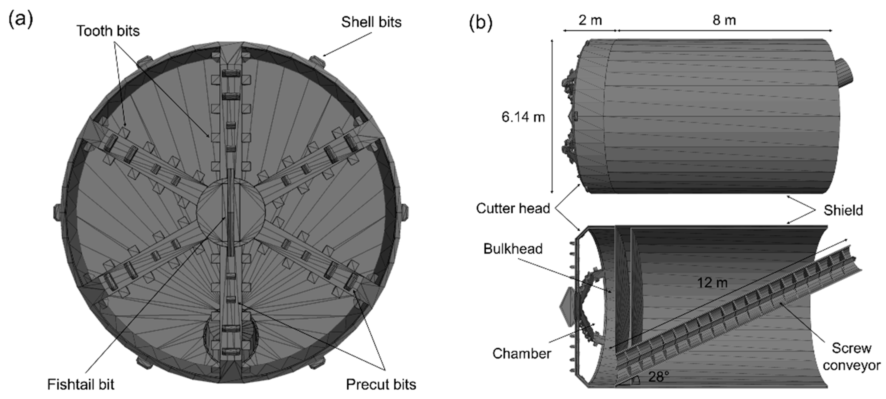
2.1. EPB Shield Model
2.2. Calibration of Contact Parameters
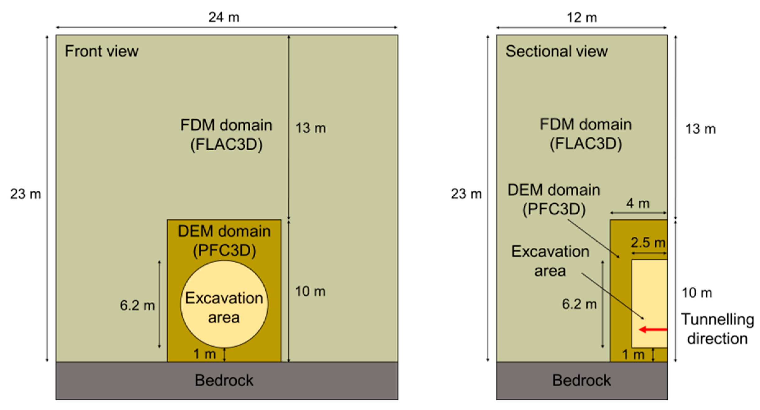
2.3. Ground Formation with Coupled Discrete Element Method-Finite Difference Method (DEM-FDM)
- (1)
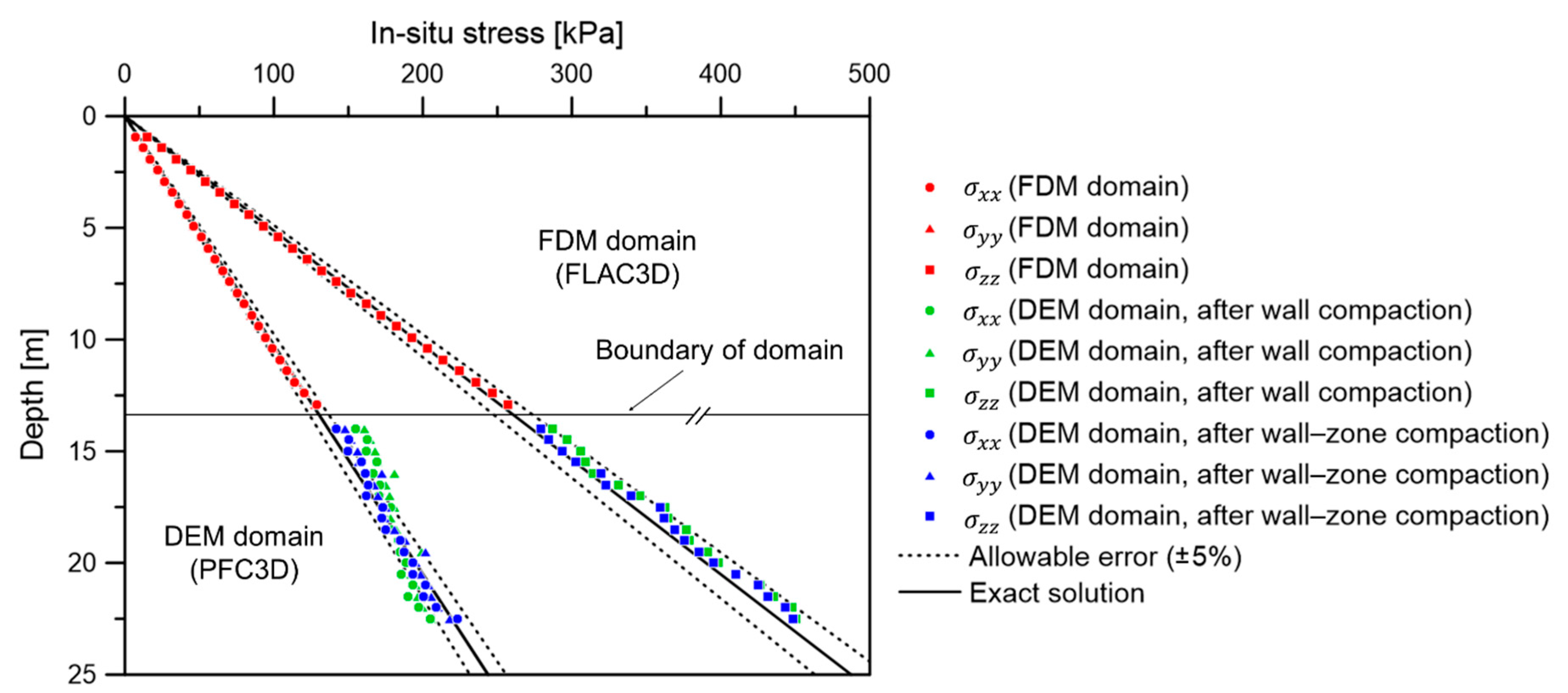
- Wall compaction. Within the specified DEM domain, after the ball elements are generated using the conditions determined by preliminary calibration (Table 5), 6 walls (12 facets) are installed around the ball assembly. Excluding the side where tunnelling is initiated and the bottom wall, the designated loads are applied through five walls (one top and four side walls) with a servo-mechanism. On the top wall, vertical earth pressure is loaded considering the cover depth. On the four side walls, the average lateral earth pressure is applied considering the lateral earth pressure coefficient at rest ( = 0.5; Figure 6a,b).
- (2)
- Wall–zone compaction. Zone elements are generated around wall-compacted balls to simulate the rest domain of the ground formation. Along zone faces of the FDM and DEM domain boundaries (i.e., wall–zone boundaries), walls are created by wrapping zone faces. After that, input parameters (Table 5) are applied to zones and time-stepping is conducted with gravitational acceleration until the convergence criterion is satisfied. During wall–zone compaction, a quarter of the target elastic modulus ( = 6 MPa) is applied as zones should be sufficiently deformed to guarantee efficient transmission of stress into the DEM domain. Upon completion of ground stabilization, the elastic modulus is modified to the designated value ( = 24 MPa; Figure 6c,d).
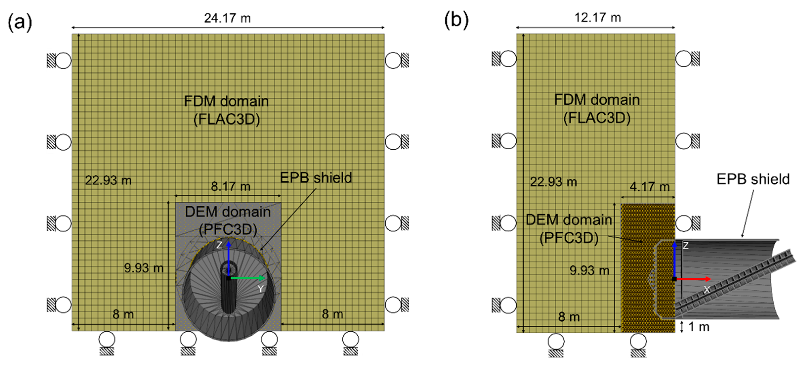
2.4. Numerical Model and Analysis
3. Discussion of Analysis Results
3.1. Torque and Thrust Force
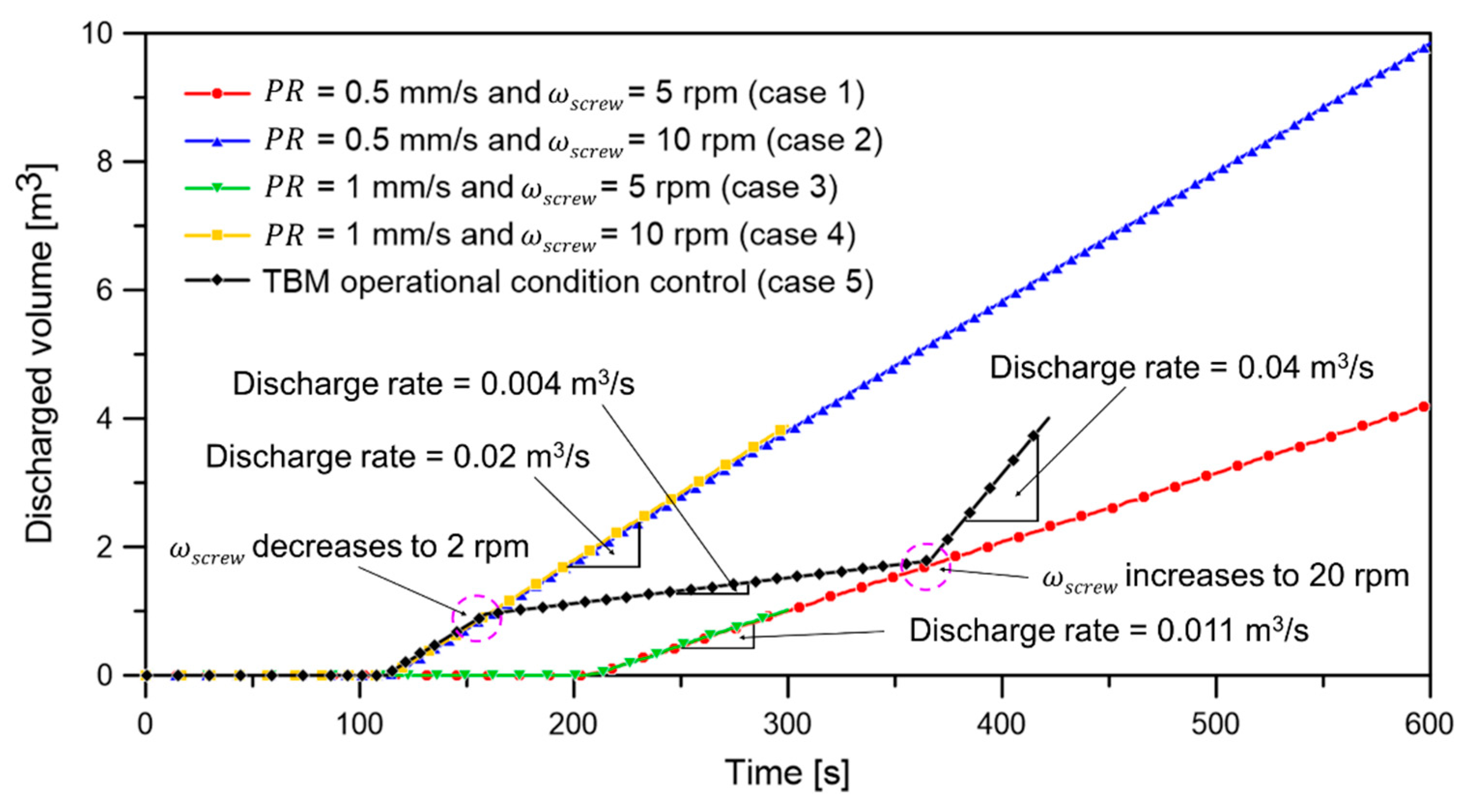
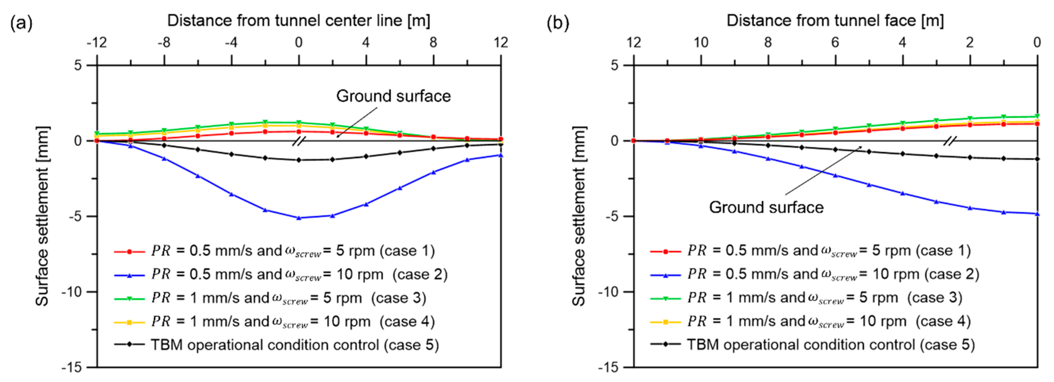
3.2. Chamber Pressure, Discharge, and Surface Settlement
4. Conclusions
- The numerical model successfully simulated EPB shield tunnelling under control of the operational conditions. During an advance of 300 mm, the penetration rate and rotational speed of the screw conveyor were varied four times in response to the monitored TBM data. The adjustments ensured that the measured torque, thrust force, and chamber pressure remained within their specified operational ranges.
- The simulated torque and thrust force data demonstrated the significance of adopting appropriate penetration rate and rotational speed of the screw conveyor to enhancing the TBM performance. When the torque and thrust force were maintained within their specified operational ranges, the TBM advance was optimal within its specifications.
- The chamber pressure and discharge data were directly related to the safety of tunnelling. Insufficient or excessive chamber pressure could induce surface settlement or heaving. However, controlling the chamber pressure and discharge during operation considerably suppressed surface settlement. Therefore, maintaining appropriate chamber pressure and muck discharge is significant for safe tunnelling with an EPB shield.
- The provided numerical model could be a useful tool for gathering simulated real-time TBM data and finding the optimal TBM operational conditions for efficient and safe tunnelling. In future, with some modifications, the model can be used in automatic TBM driving, simulating multiple-layer soil tunnelling, and designing cutter heads.
Author Contributions
Funding
Informed Consent Statement
Data Availability Statement
Acknowledgments
Conflicts of Interest
References
- Bavasso, I.; Vilardi, G.; Sebastiani, D.; Di Giulio, A.; Di Felice, M.; Di Biase, A.; Miliziano, S.; Di Palma, L. A rapid experimental procedure to assess environmental compatibility of conditioning mixtures used in TBM-EPB technology. Appl. Sci. 2020, 10, 4138. [Google Scholar] [CrossRef]
- Xu, Q.; Zhang, L.; Zhu, H.; Gong, Z.; Liu, J.; Zhu, Y. Laboratory tests on conditioning the sandy cobble soil for EPB shield tunnelling and its field application. Tunn. Undergr. Space Technol. 2020, 105, 103512. [Google Scholar] [CrossRef]
- Hammerer, N. Influence of Steering Actions by the Machine Operator on the Interpretation of TBM Performance Data; University of Innsbruck: Innsbruck, Austria, 2015. [Google Scholar]
- Yamamoto, T.; Shirasagi, S.; Yamamoto, S.; Mito, Y.; Aoki, K. Evaluation of the geological condition ahead of the tunnel face by geostatistical techniques using TBM driving data. Mod. Tunn. Sci. Technol. 2017, 1, 213–218. [Google Scholar] [CrossRef]
- Festa, D.; Broere, W.; Bosch, J.W. An investigation into the forces acting on a TBM during driving—Mining the TBM logged data. Tunn. Undergr. Space Technol. 2012, 32, 143–157. [Google Scholar] [CrossRef]
- Chakeri, H.; Hasanpour, R.; Hindistan, M.A.; Ünver, B. Analysis of interaction between tunnels in soft ground by 3D numerical modeling. Bull. Eng. Geol. Environ. 2011, 70, 439–448. [Google Scholar] [CrossRef]
- Lambrughi, A.; Medina Rodríguez, L.; Castellanza, R. Development and validation of a 3D numerical model for TBM-EPB mechanised excavations. Comput. Geotech. 2012, 40, 97–113. [Google Scholar] [CrossRef]
- Mancinelli, D.L. Evaluation of superficial settlements in low overburden tunnel TBM excavation: Numerical approaches. Geotech. Geol. Eng. 2005, 23, 263–271. [Google Scholar] [CrossRef]
- Lu, C.C.; Hwang, J.H. Implementation of the modified cross-section racking deformation method using explicit FDM program: A critical assessment. Tunn. Undergr. Space Technol. 2017, 68, 58–73. [Google Scholar] [CrossRef]
- Nikakhtar, L.; Zare, S.; Nasirabad, H.M.; Ferdosi, B. Application of ANN-PSO algorithm based on FDM numerical modelling for back analysis of EPB TBM tunneling parameters. Eur. J. Environ. Civ. Eng. 2020, 1–18. [Google Scholar] [CrossRef]
- Kasper, T.; Meschke, G. A 3D finite element simulation model for TBM tunnelling in soft ground. Int. J. Numer. Anal. Methods Geomech. 2004, 28, 1441–1460. [Google Scholar] [CrossRef]
- Liu, C.; Peng, Z.; Pan, L.; Liu, H.; Yang, Y.; Chen, W.; Jiang, H. Influence of tunnel boring machine (TBM) advance on adjacent tunnel during ultra-rapid underground pass (URUP) tunneling: A case study and numerical investigation. Appl. Sci. 2020, 10, 3746. [Google Scholar] [CrossRef]
- Kim, K.; Oh, J.; Lee, H.; Kim, D.; Choi, H. Critical face pressure and backfill pressure in shield TBM tunneling on soft ground. Geomech. Eng. 2018, 15, 823–831. [Google Scholar] [CrossRef]
- Han, M.D.; Cai, Z.X.; Qu, C.Y.; Jin, L.S. Dynamic numerical simulation of cutterhead loads in TBM tunnelling. Tunn. Undergr. Space Technol. 2017, 70, 286–298. [Google Scholar] [CrossRef]
- Dang, T.S.; Meschke, G. A Shear-Slip Mesh Update—Immersed Boundary Finite Element model for computational simulations of material transport in EPB tunnel boring machines. Finite Elem. Anal. Des. 2018, 142, 1–16. [Google Scholar] [CrossRef]
- Zhu, H.; Panpan, C.; Xiaoying, Z.; Yuanhai, L.; Peinan, L. Assessment and structural improvement on the performance of soil chamber system of EPB shield assisted with DEM modeling. Tunn. Undergr. Space Technol. 2020, 96, 103092. [Google Scholar] [CrossRef]
- Jiang, M.; Yin, Z.Y. Analysis of stress redistribution in soil and earth pressure on tunnel lining using the discrete element method. Tunn. Undergr. Space Technol. 2012, 32, 251–259. [Google Scholar] [CrossRef]
- Zhang, Z.; Zhang, X.; Sun, S.; Liang, Z. A cross-river tunnel excavation considering the water pressure effect based on DEM. Eur. J. Environ. Civ. Eng. 2019, 1–17. [Google Scholar] [CrossRef]
- Zhang, Z.X.; Hu, X.Y.; Scott, K.D. A discrete numerical approach for modeling face stability in slurry shield tunnelling in soft soils. Comput. Geotech. 2011, 38, 94–104. [Google Scholar] [CrossRef]
- Cundall, P.A. A computer model for simulating progressive, large-scale movement in blocky rock system. In Proceedings of the International Symposium on Rock Mechanics, Nancy, France, 4–6 October 1971. [Google Scholar]
- Cundall, P.A.; Strack, O.D.L. A discrete numerical model for granular assemblies. Geotechnique 1979, 29, 47–65. [Google Scholar] [CrossRef]
- Faramarzi, L.; Kheradmandian, A.; Azhari, A. Evaluation and optimization of the effective parameters on the shield TBM performance: Torque and thrust—Using discrete element method (DEM). Geotech. Geol. Eng. 2020, 38, 2745–2759. [Google Scholar] [CrossRef]
- Maynar, M.J.; Rodríguez, L.E. Discrete numerical model for analysis of earth pressure balance tunnel excavation. J. Geotech. Geoenviron. Eng. 2005, 131, 1234–1242. [Google Scholar] [CrossRef]
- Wu, L.; Guan, T.; Lei, L. Discrete element model for performance analysis of cutterhead excavation system of EPB machine. Tunn. Undergr. Space Technol. 2013, 37, 37–44. [Google Scholar] [CrossRef]
- Wang, J.; He, C.; Xu, G. Face stability analysis of EPB shield tunnels in dry granular soils considering dynamic excavation process. J. Geotech. Geoenviron. Eng. 2019, 145, 1–10. [Google Scholar] [CrossRef]
- Chen, R.P.; Tang, L.J.; Ling, D.S.; Chen, Y.M. Face stability analysis of shallow shield tunnels in dry sandy ground using the discrete element method. Comput. Geotech. 2011, 38, 187–195. [Google Scholar] [CrossRef]
- Cho, N.; Martin, C.D.; Sego, D.C. A clumped particle model for rock. Int. J. Rock Mech. Min. Sci. 2007, 44, 997–1010. [Google Scholar] [CrossRef]
- Yang, S.Q.; Chen, M.; Fang, G.; Wang, Y.C.; Meng, B.; Li, Y.H.; Jing, H.W. Physical experiment and numerical modelling of tunnel excavation in slanted upper-soft and lower-hard strata. Tunn. Undergr. Space Technol. 2018, 82, 248–264. [Google Scholar] [CrossRef]
- Hu, X.; He, C.; Lai, X.; Walton, G.; Fu, W.; Fang, Y. A DEM-based study of the disturbance in dry sandy ground caused by EPB shield tunneling. Tunn. Undergr. Space Technol. 2020, 101, 103410. [Google Scholar] [CrossRef]
- Chen, S.G.; Zhao, J. Modeling of tunnel excavation using a hybrid DEM/BEM method. Comput. Civ. Infrastruct. Eng. 2002, 17, 381–386. [Google Scholar] [CrossRef]
- Manolis, G.D.; Parvanova, S.L.; Makra, K.; Dineva, P.S. Seismic response of buried metro tunnels by a hybrid FDM-BEM approach. Bull. Earthq. Eng. 2015, 13, 1953–1977. [Google Scholar] [CrossRef]
- Zhao, J.; Shan, T. Coupled CFD-DEM simulation of fluid-particle interaction in geomechanics. Powder Technol. 2013, 239, 248–258. [Google Scholar] [CrossRef]
- Zhao, X.; Xu, J.; Zhang, Y.; Xiao, Z. Coupled DEM and FDM algorithm for geotechnical analysis. Int. J. Geomech. 2018, 18, 04018040. [Google Scholar] [CrossRef]
- Wu, Z.; Zhang, P.; Fan, L.; Liu, Q. Numerical study of the effect of confining pressure on the rock breakage efficiency and fragment size distribution of a TBM cutter using a coupled FEM-DEM method. Tunn. Undergr. Space Technol. 2019, 88, 260–275. [Google Scholar] [CrossRef]
- Labra, C.; Rojek, J.; Oñate, E. Discrete/finite element modelling of rock cutting with a TBM disc cutter. Rock Mech. Rock Eng. 2017, 50, 621–638. [Google Scholar] [CrossRef]
- Yin, Z.Y.; Wang, P.; Zhang, F. Effect of particle shape on the progressive failure of shield tunnel face in granular soils by coupled FDM-DEM method. Tunn. Undergr. Space Technol. 2020, 100, 103394. [Google Scholar] [CrossRef]
- Qu, T.; Wang, S.; Hu, Q. Coupled discrete element-finite difference method for analysing effects of cohesionless soil conditioning on tunneling behaviour of EPB shield. KSCE J. Civ. Eng. 2019, 23, 4538–4552. [Google Scholar] [CrossRef]
- Itasca Consulting Group Inc. Fast Lagrangian Analysis of Continua in Three Dimensions (FLAC3D), version 7.0; Itasca Consulting Group: Minneapolis, MN, USA, 2020. [Google Scholar]
- Itasca Consulting Group Inc. Particle Flow Code in Three Dimensions (PFC3D), version 6.0; Itasca Consulting Group: Minneapolis, MN, USA, 2020. [Google Scholar]
- Shen, Z.; Jiang, M.; Thornton, C. DEM simulation of bonded granular material. Part I: Contact model and application to cemented sand. Comput. Geotech. 2016, 75, 192–209. [Google Scholar] [CrossRef]
- Moon, T.; Oh, J. A study of optimal rock-cutting conditions for hard rock TBM using the discrete element method. Rock Mech. Rock Eng. 2012, 45, 837–849. [Google Scholar] [CrossRef]
- Potyondy, D.O.; Cundall, P.A. A bonded-particle model for rock. Int. J. Rock Mech. Min. Sci. 2004, 41, 1329–1364. [Google Scholar] [CrossRef]
- Potyondy, D.O. The bonded-particle model as a tool for rock mechanics research and application: Current trends and future directions. Geosystem Eng. 2015, 18, 1–28. [Google Scholar] [CrossRef]
- Gilabert, F.A.; Roux, J.N.; Castellanos, A. Computer simulation of model cohesive powders: Plastic consolidation, structural changes, and elasticity under isotropic loads. Phys. Rev. E Stat. Nonlinear Soft Matter Phys. 2008, 78, 1–21. [Google Scholar] [CrossRef]
- Gilabert, F.A.; Roux, J.N.; Castellanos, A. Computer simulation of model cohesive powders: Influence of assembling procedure and contact laws on low consolidation states. Phys. Rev. E Stat. Nonlinear Soft Matter Phys. 2007, 75, 1–26. [Google Scholar] [CrossRef] [PubMed]
- Cil, M.B.; Alshibli, K.A. 3D analysis of kinematic behavior of granular materials in triaxial testing using DEM with flexible membrane boundary. Acta Geotech. 2014, 9, 287–298. [Google Scholar] [CrossRef]
- Qu, T.; Feng, Y.T.; Wang, Y.; Wang, M. Discrete element modelling of flexible membrane boundaries for triaxial tests. Comput. Geotech. 2019, 115, 103154. [Google Scholar] [CrossRef]
- Shi, H.; Yang, H.; Gong, G.; Wang, L. Determination of the cutterhead torque for EPB shield tunneling machine. Autom. Constr. 2011, 20, 1087–1095. [Google Scholar] [CrossRef]
- Reilly, B.J. EPBMs for the North East Line Project. Tunn. Undergr. Space Technol. 1999, 14, 491–508. [Google Scholar] [CrossRef]
- Ates, U.; Bilgin, N.; Copur, H. Estimating torque, thrust and other design parameters of different type TBMs with some criticism to TBMs used in Turkish tunneling projects. Tunn. Undergr. Space Technol. 2014, 40, 46–63. [Google Scholar] [CrossRef]
- Zizka, Z.; Thewes, M. Recommendations for Face Support Pressure Calculations for Shield Tunnelling in Soft Ground; DAUB: Cologne, Germany, 2016. [Google Scholar]


| Property | Value |
|---|---|
| Type of soil | Weathered granite soil |
| Dry unit weight [kN/m3] | 19.5 |
| Internal friction angle, [°] | 27.3 |
| Cohesion, [kPa] | 26.3 |
| Lateral earth pressure coefficient at rest, [-] | 0.5 |
| Thickness of soil layer [m] | 23 |
| Cover depth [m] | 15.8 |
| Diameter of excavation area [m] | 6.2 |
| Property | Value |
|---|---|
| Type of cutter head | Spoke-type |
| Diameter of cutter head [m] | 6.14 |
| Number of spokes | 6 |
| Number of cutting tools | 91 |
| Opening ratio [%] | 75.5 |
| Type of screw conveyor | Shaft-type |
| Diameter of screw [m] | 0.9 |
| Length of screw conveyor [m] | 12 |
| Pitch of screw [m] | 0.5 |
| Inclination of screw conveyor [°] | 28 |
| Length of shield [m] | 8 |
| Property | Value |
|---|---|
| Dimension of specimen, × [m] | 2 × 4 |
| Packing of ball element | Hexagonal close packing |
| Diameter of ball element [cm] | 20 |
| Number of ball element | 2101 |
| Density of ball element [kg/m3] | 2700 |
| Contact model | Adhesive rolling resistance linear |
| Number of shell element | 576 |
| Thickness of shell element [mm] | 6 |
| Density of shell element [kg/m3] | 90 |
| Elastic modulus of shell element [kPa] | 1400 |
| Confining pressure [kPa] | 125, 250, 375, 500 |
| Strain rate [%/min] | 0.03 |
| Calibrated Contact Parameters of Adhesive Rolling Resistance Linear Contact Model | ||||
| Parameter | Value | |||
| Normal stiffness, [MN/m] | 4.5 | |||
| Shear stiffness, [MN/m] | 3 | |||
| Friction coefficient, [-] | 0.07 | |||
| Reference gap, [mm] | 0 | |||
| Effective modulus, [MN/m2] | 10 | |||
| Rolling friction coefficient, [-] | 0.03 | |||
| Normal critical damping ratio, [-] | 0.05 | |||
| Shear critical damping ratio, [-] | 0.05 | |||
| Maximum attractive force, [N] | 0.01 | |||
| Attraction range, [mm] | 2.5 | |||
| Calibrated Mohr–Coulomb Failure Criterion Parameters | ||||
| Parameter | Calibrated Value | Target Value | Error [%] | |
| Internal friction angle, [°] | 27.22 | 27.3 | 0.29 | |
| Cohesion, [kPa] | 26.17 | 26.3 | 0.49 | |
| DEM Domain | |
| Property | Value |
| Packing of ball element | Hexagonal close packing |
| Diameter of ball element [m] | 0.1 |
| Number of ball element | 59,024 |
| Density of ball element [kg/m3] | 2700 |
| Contact model of ball element | Adhesive rolling resistance linear |
| Contact parameters | Refer to Table 4 |
| FDM Domain | |
| Property | Value |
| Size of zone element, × [m] | 0.5 × 0.5 |
| Number of zone element | 50,432 |
| Density of zone element [kg/m3] | 1987.77 |
| Constitutive model of zone element | Mohr–Coulomb failure criterion |
| Elastic modulus, [MPa] | 24 |
| Poisson’s ratio, [-] | 0.3 |
| Internal friction angle, [°] | 27.3 |
| Cohesion, [kPa] | 26.3 |
| Lateral earth pressure coefficient at rest, [-] | 0.5 |
| Case Number | Rotational Speed of Cutter Head, [rpm] | Penetration Rate, PR [mm/s] | Rotational Speed of Screw Conveyor, [rpm] |
|---|---|---|---|
| 1 | 2 | 0.5 | 5 |
| 2 | 10 | ||
| 3 | 1 | 5 | |
| 4 | 10 | ||
| 5 | Automatically controlled (initial = 0.5 mm/s and = 10 rpm) | ||
| Advance [mm] | Time [s] | Penetration Rate, PR [mm/s] | Rotational Speed of Screw Conveyor, [rpm] | Note |
|---|---|---|---|---|
| 0 | 0 | 0.5 | 10 | Initiation of tunnelling |
| 48.96 | 97.92 | 2 | 10 | Lower bound of thrust force |
| 164.15 | 155.52 | 2 | 2 | Lower bound of chamber pressure |
| 255.69 | 201.29 | 0.2 | 2 | Upper bound of torque |
| 287.87 | 362.19 | 0.2 | 20 | Upper bound of chamber pressure |
| 300 | 422.84 | 0.2 | 20 | End of tunnelling |
Publisher’s Note: MDPI stays neutral with regard to jurisdictional claims in published maps and institutional affiliations. |
© 2021 by the authors. Licensee MDPI, Basel, Switzerland. This article is an open access article distributed under the terms and conditions of the Creative Commons Attribution (CC BY) license (http://creativecommons.org/licenses/by/4.0/).
Share and Cite
Lee, H.; Choi, H.; Choi, S.-W.; Chang, S.-H.; Kang, T.-H.; Lee, C. Numerical Simulation of EPB Shield Tunnelling with TBM Operational Condition Control Using Coupled DEM–FDM. Appl. Sci. 2021, 11, 2551. https://doi.org/10.3390/app11062551
Lee H, Choi H, Choi S-W, Chang S-H, Kang T-H, Lee C. Numerical Simulation of EPB Shield Tunnelling with TBM Operational Condition Control Using Coupled DEM–FDM. Applied Sciences. 2021; 11(6):2551. https://doi.org/10.3390/app11062551
Chicago/Turabian StyleLee, Hyobum, Hangseok Choi, Soon-Wook Choi, Soo-Ho Chang, Tae-Ho Kang, and Chulho Lee. 2021. "Numerical Simulation of EPB Shield Tunnelling with TBM Operational Condition Control Using Coupled DEM–FDM" Applied Sciences 11, no. 6: 2551. https://doi.org/10.3390/app11062551
APA StyleLee, H., Choi, H., Choi, S.-W., Chang, S.-H., Kang, T.-H., & Lee, C. (2021). Numerical Simulation of EPB Shield Tunnelling with TBM Operational Condition Control Using Coupled DEM–FDM. Applied Sciences, 11(6), 2551. https://doi.org/10.3390/app11062551